Some physical and chemical indices of clique-inserted lattices

Abstract

The operation of replacing every vertex of an $r$-regular lattice $H$ by a complete graph of order $r$ is called clique-inserting, and the resulting lattice is called the clique-inserted lattice of $H$. For any given $r$-regular lattice, applying this operation iteratively, an infinite family of $r$-regular lattices is generated. Some interesting lattices including the 3-12-12 lattice can be constructed this way. In this paper, we recall the relationship between the spectra of an $r$-regular lattice and that of its clique-inserted lattice, and investigate the graph energy and resistance distance statistics. As an application, the asymptotic energy per vertex and average resistance distance of the 3-12-12 and 3-6-24 lattices are computed. We also give formulae expressing the numbers of spanning trees and dimer coverings of the $k$-th iterated clique-inserted lattices in terms of that of the original one. Moreover, we show that new families of expander graphs can be constructed from the known ones by clique-inserting.

Keywords: Clique-inserting, Graph energy, Kirchhoff index, Dimer model, Spanning tree, Expander graphs

1 Introduction

In the study of lattice statistical physics, one family of $2$-dimensional lattices that have received a lot of attention are constructed by replacing each vertex of $r$-regular lattices with a complete graph of order $r$ such that each of the $r$ new vertices corresponds to one of the incident edges. (To avoid triviality, we assume $r\geq 3$ throughout the paper.) Such lattices include the martini [18, 23, 21], the 3-12-12 [19, 22, 21], the 3-6-24 [6] and the modified bath room lattices [21]. Following [29], the operation of transforming each vertex of an $r$-regular graph to an $r$-clique (complete graph of order $r$) is called clique-inserting, and the graph obtained this way is called the clique-inserted graph of the original graph. From a given $r$-regular lattice $H$, the operation of clique-inserting can also be performed, and the resulting lattice $C(H)$ is called the clique-inserted lattice of the original lattice.

Throughout this paper, we always assume that $G$ denotes an undirected simple graph. Note that in the language of graph theory, the clique-insertion operation on a graph $G$ can be described as taking the line graph of the subdivision graph of $G$. For any given regular lattice $H$, by iterating this operation, a set of hierarchical regular lattices, namely, iterated clique-inserted lattices can be obtained. Denote $\{C^{k}(H)\}_{k\geq 0}$ the sequence of clique-inserted lattices with $C^{0}(H)\equiv H$ and $C^{k+1}(H)=C(C^{k}(H))$. Start with the hexagonal lattice, the 3-12-12, 3-6-24 and 3-6-12-48 lattices (refer to [6] for definitions of these lattices) can be generated by clique-inserting. In this case, the clique-insertion operation on a lattice is equivalent to the fundamental “Y-Delta” transformation (also known as the star-triangle transformation) on the subdivision graph of the original lattice. By this observation we obtained the relations between some physical and chemical indices of $r$-regular lattices and their $k$-th clique-inserted lattices. With such relations, we can compute some indices of some complex lattices easily based on the results of well-studied lattices such as the square and hexagonal lattices.

In this paper, we consider the lattices produced by the operation of clique-inserting on regular lattices with free, cylindrical and toroidal boundary conditions. We will discuss the energy per vertex, average resistance (the Kirchhoff index over the number of pairs of vertices) and the entropy of spanning-tree and dimer models of such lattices. We will also use the operation of clique-inserting to construct new families of expander graphs from known ones.

The dimer model on regular lattices has attracted the attention of many physicists as well as mathematicians. For some classical works, we refer to [20, 4, 22]. Cayley[1] and Kirchhoff[11] presented the problem of enumeration of spanning trees of graphs, and further work in statistical physics has appeared in both physics and mathematics literature. For a good survey, the reader is referred to [19]. On the basis of electrical network theory, the study of resistance distance was initiated by Klein and Randić[12], and the related index named “Kirchhoff index” was well studied in [9, 24]. In 1930s, Hückel proposed a method for finding approximate solution of the Schrödinger equation of a class of organic molecules, the so-called conjugated hydrocarbons. In the framework of this modelization, the total $\pi$-electron energy, can be approximated by the sum of the absolute values of eigenvalues of the molecular graphs under certain chemical-based conditions. Gutman abstracted a mathematical notion from this application-driven analysis on molecular graphs, therefore he defined graph energy as a graph invariant[7, 8]. Since then, graph energy has been studied extensively by Chemists and Mathematicians. Yan and Zhang [27] proposed the energy per vertex problem for lattice systems and showed that the energy per vertex of 2-dimensional lattices is independent from the boundary conditions, under various choices. For a comprehensive survey of results and common proof methods obtained on graph energy, see the monograph on graph energy [13] and references cited therein. Expander graphs were first defined by Bassalygo and Pinsker in the early 70’s. These graphs are regular sparse graphs with strong connectivity properties, measured by vertex, edge or spectral expansion as described in [10]. For a graph, having such a property has significant implications in various disciplines including complexity theory, computer networks, statistical mechanics and so on.

The rest of the paper is organized as follows. The expression of the energy and Kirchhoff index of $k$-th iterated clique-inserted lattices of regular lattices are discussed in sections $2$ and $3$, respectively. As an application, we compute the energy per vertex and average Kirchhoff index of the 3-12-12 and 3-6-24 lattices. In Section $4$, we show that, given $z_{H}$ as the entropy of spanning trees of an $r$-regular lattice $H$, the entropy of spanning trees of $C^{k}(H)$ (the $k$-th iterated clique-inserted graph of $H$) is given by $r^{-k}(z_{H}+s_{k}(r)\ln{r(r+2)})$ where $s_{k}(r)=(r/2-1)(r^{k}-1)/(r-1)$. We will also show that when $H$ is cubic, the free energy per dimer of $C^{k}(H)$ is $\frac{1}{3}\ln{2}$. In Section $5$, inspired by the Liu and Zhou’s work [14], we show that by applying clique-insertion operation iteratively on an expander family, new families of expander graphs can be obtained. We propose clique-inserting as a modification to extend the size of computer networks, with their expansion properties being preserved to a certain degree.

2 Asymptotic Energy

Let $G=(V(G),E(G))$ be a graph with vertex set $V(G)=\{v_{1},v_{2},\ldots,v_{n}\}$ and edge set $E(G)$. The adjacency matrix of $G$, denoted by $A(G)$, is the $n\times n$ symmetric matrix such that $a_{ij}=1$ if vertices $v_{i}$ and $v_{j}$ are adjacent and $0$ otherwise. Let $d_{G}(v_{i})$ be the degree of vertex $v_{i}$ of $G$. The Line graph $L(G)$ of $G$, is the graph such that each vertex of $L(G)$ represents an edge of $G$ and two vertices of $L(G)$ are adjacent if and only if their corresponding edges of $G$ share a common end vertex in $G$. The subdivision graph $S(G)$ of a graph $G$ is the graph obtained by inserting a new vertex into every edge of $G$. It is easy to see that $C(G)=L(S(G))$. The energy of a graph $G$ with $n$ vertices, denoted by $\mathcal{E}(G)$, is defined by $\mathcal{E}(G)=\sum_{i=1}^{n}|\lambda_{i}(G)|$, where $\lambda_{i}(G)$’s are the eigenvalues of the adjacency matrix of $G$. The asymptotic energy per vertex of $G$ [27] is defined by $\lim\limits_{|V(G)|\rightarrow\infty}\frac{\mathcal{E}(G)}{|V(G)|}$.

Lemma 2.1.

[27] Suppose that $\{G_{n}\}$ is a sequence of finite simple graphs with bounded average degree such that $\lim\limits_{n\rightarrow\infty}|V(G_{n})|=\infty$ and $\lim\limits_{n\rightarrow\infty}\frac{\mathcal{E}(G_{n})}{|V(G_{n})|}=h\neq 0$. If $\{G_{n}^{\prime}\}$ is a sequence of spanning subgraphs of $\{G_{n}\}$ such that $\lim\limits_{n\rightarrow\infty}\frac{|\{v\in V(G_{n}^{\prime}):d_{G_{n}^{\prime}}(v)=d_{G_{n}}(v)\}|}{|V(G_{n})|}=1$, then $\lim\limits_{n\rightarrow\infty}\frac{\mathcal{E}(G^{\prime}_{n})}{|V(G_{n}^{\prime})|}=h$. That is, $G_{n}$ and $G_{n}^{\prime}$ have the same asymptotic energy.

Lemma 2.2.

[29] Let $G$ be an $r$-regular graph with $n$ vertices and $m$ edges. Suppose that the eigenvalues of $G$ are $\lambda_{1}$ = $r\geq\lambda_{2}\geq...\geq\lambda_{n}$. Then the eigenvalues of the clique-inserted graph $C(G)$ of $G$ are $\frac{r-2\pm\sqrt{r^{2}+4(\lambda_{i}+1)}}{2}$, $i=1,2,...,n$, besides $-2$ and $0$ each with multiplicity $m-n$.

From Lemma 2.2, we immediately obtain the following corollary.

Corollary 2.3.

Let $G$ be an $r$-regular $(r\geq 3)$ graph with $n$ vertices and eigenvalues $\lambda_{1}\geq\lambda_{2}\geq...\geq\lambda_{n}$, the energy of the clique-inserted graph of $G$ is

$$\mathcal{E}(C(G))=\sum_{i=1}^{n}\sqrt{r^{2}+4(\lambda_{i}+1)}+n.$$

We will use this result to calculate the asymptotic energy per vertex of the 3-12-12 lattice and its clique-inserted lattice in the rest of this section.

2.1 3-12-12 lattice

Our notation for the hexagonal lattices follows [27]. The hexagonal lattices on a $n\times m$ torus, denoted by $H^{t}(n,m)$, are illustrated in Figure 1, where $(a_{1},a^{*}_{1}),(a_{2},a^{*}_{2}),\ldots,(a_{m+1},a^{*}_{m+1})$, $(b_{1},b^{*}_{1}),(b_{2},b^{*}_{2}),\\ \ldots,(b_{n+1},b^{*}_{n+1})$ are edges in $H^{t}(n,m)$.

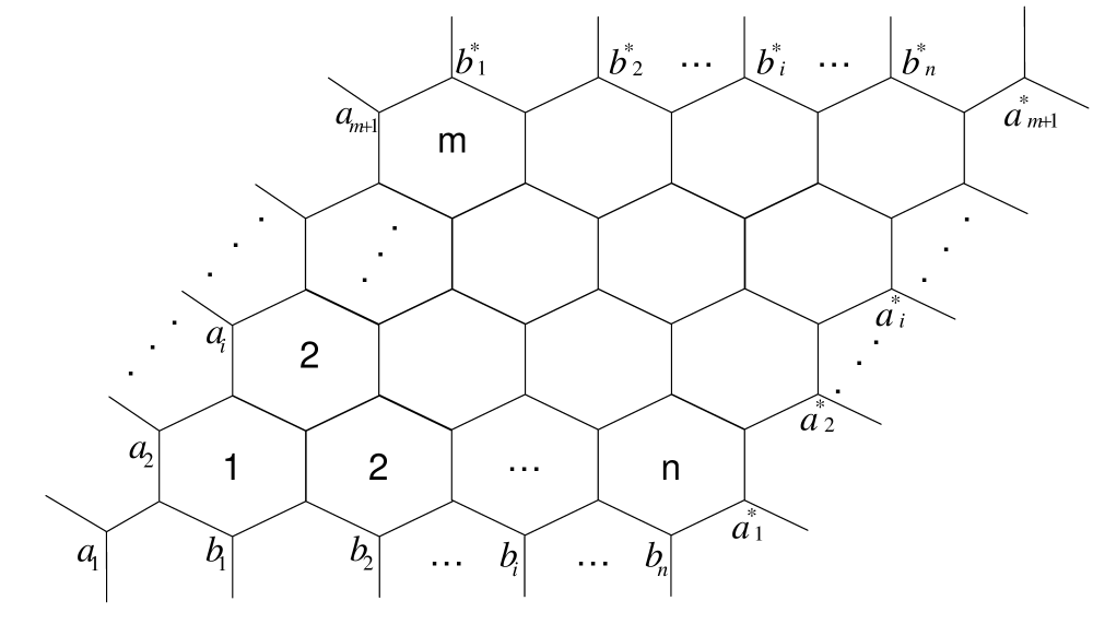
Fig. 1: $H^{t}(n,m)$ with toroidal boundary condition

By the definition of a clique-inserted lattice, it is easy to see that each 3-12-12 lattice on the same geometry is a clique-inserted-graph of $H^{t}(n,m)$, denoted as $T^{t}(n,m)$ (see Figure 2(a)). Note that $(a_{1},a^{*}_{1}),(a_{2},a^{*}_{2}),\ldots,(a_{m+1},a^{*}_{m+1})$, $(b_{1},b^{*}_{1}),(b_{2},b^{*}_{2}),\ldots,(b_{n+1},b^{*}_{n+1})$ are edges in $T^{t}(m,n)$. If we delete edges $(b_{1},b^{*}_{1}),(b_{2},b^{*}_{2}),\ldots,(b_{n+1},b^{*}_{n+1})$ from $T^{t}(n,m)$, then the 3-12-12 lattice with cylindrical boundary condition, denoted by $T^{c}(n,m)$ (see Figure 2(b)) can be obtained. If we delete the edges $(a_{1},a^{*}_{1}),(a_{2},a^{*}_{2}),\ldots,(a_{m+1},a^{*}_{m+1})$ from $T^{c}(m,n)$, then the 3-12-12 lattice with free boundary condition, denoted by $T^{f}(m,n)$ (see Figure 2(c)) can be obtained.

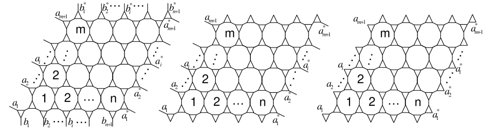
Fig. 2:  The 3-12-12 lattice $T^{t}(n,m)$ (left), $T^{c}(n,m)$ (middle), and $T^{f}(n,m)$.

Note that almost all vertices of $T^{c}(m,n)$ and $T^{f}(m,n)$ are of degree $3$. Since $T^{f}(m,n)$ and $T^{c}(m,n)$ are spanning subgraphs of $T^{t}(m,n)$, by Lemma 2.1 we have

$$\lim_{n,m\rightarrow\infty}\frac{\mathcal{E}(T^{t}(n,m))}{6mn}=\lim_{n,m\rightarrow\infty}\frac{\mathcal{E}(T^{c}(n,m))}{6mn}=\lim_{n,m\rightarrow\infty}\frac{\mathcal{E}(T^{f}(n,m))}{6mn}$$

It is shown in [27] that the eigenvalues of $H^{t}(n,m)$ are:

$$\pm\sqrt{3+2\cos\frac{2i\pi}{n+1}+2\cos\frac{2j\pi}{m+1}+2\cos\left(\frac{2i\pi}{n+1}+\frac{2j\pi}{m+1}\right)},0\leq i\leq n,0\leq j\leq m.$$

Since $T^{t}(n,m)$ is the clique-inserted graph of $H^{t}(n,m)$, we have

$$\mathcal{E}(T^{t}(n,m)) = \sum\limits_{i=0}^{n}\sum\limits_{j=0}^{m}\sqrt{13+4\sqrt{3+2\cos\frac{2i\pi}{n+1}+2\cos\frac{2j\pi}{m+1}+2\cos\left(\frac{2i\pi}{n+1}+\frac{2j\pi}{m+1}\right)}}$$

$$+\sum\limits_{i=0}^{n}\sum\limits_{j=0}^{m}\sqrt{13-4\sqrt{3+2\cos\frac{2i\pi}{n+1}+2\cos\frac{2j\pi}{m+1}+2\cos\left(\frac{2i\pi}{n+1}+\frac{2j\pi}{m+1}\right)}}+2mn$$

$$= \sum\limits_{i=0}^{n}\sum\limits_{j=0}^{m}\sqrt{26+2\sqrt{121-32\cos\frac{2i\pi}{n+1}-32\cos\frac{2j\pi}{m+1}-32\cos\left(\frac{2i\pi}{n+1}+\frac{2j\pi}{m+1}\right)}}+2mn.$$

Thus, the average energy per vertex of 3-12-12 lattice can be expressed as

$$\lim_{n,m\rightarrow\infty}\frac{\mathcal{E}(T^{t}(n,m))}{6mn} = \frac{1}{3}+\frac{1}{24\pi^{2}}\int_{0}^{2\pi}\int_{0}^{2\pi}\sqrt{26+2\sqrt{121-32\cos x-32\cos y-32\cos(x+y)}}{dx}{dy}$$

$$= 1.4825....$$

The last line follows by a numerical integration. Therefore, the 3-12-12 lattices $T^{t}(n,m),T^{c}(n,m)$, and $T^{f}(n,m)$ with toroidal, cylindrical, and free boundary conditions have the same asymptotic energy ($\approx 8.895mn$).

2.2 3-6-24 lattice

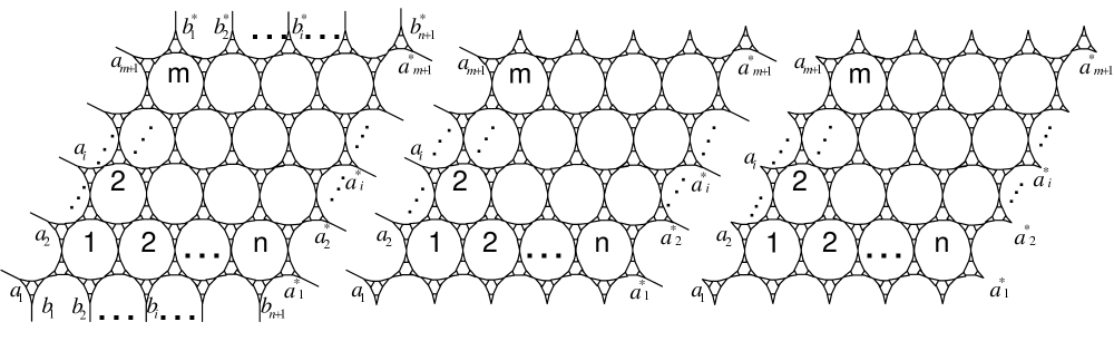
Fig. 3:  The 3-6-24 lattice $S^{t}(n,m)$ (left), $S^{c}(n,m)$ (middle), and $S^{f}(n,m)$ .

The clique-inserted lattice of $T^{t}(m,n)$ is a lattice with toroidal boundary condition, denoted by $S^{t}(m,n)$, illustrated in Figure 3. Note that $(a_{1},a^{*}_{1}),(a_{2},a^{*}_{2}),\ldots,(a_{m+1},a^{*}_{m+1})$, $(b_{1},b^{*}_{1}),(b_{2},b^{*}_{2}),\\ \ldots,(b_{n+1},b^{*}_{n+1})$ are edges in $S^{t}(m,n)$. If we delete edges $(b_{1},b^{*}_{1}),(b_{2},b^{*}_{2}),\ldots,(b_{n+1},b^{*}_{n+1})$ from $S^{t}(n,m)$, then the 3-6-24 lattice with cylindrical boundary condition, denoted by $S^{c}(n,m)$ (see Figure 3(b)) can be obtained. If we delete edges $(a_{1},a^{*}_{1}),(a_{2},a^{*}_{2}),\ldots,(a_{m+1},a^{*}_{m+1})$ from $S^{c}(m,n)$, then the 3-6-24 lattice with free boundary condition, denoted by $S^{f}(m,n)$ (see Figure 3(c)) can be obtained.

Note that $S^{f}(m,n)$ and $S^{c}(m,n)$ are spanning subgraphs of $S^{t}(m,n)$, by Lemma 2.1 we have

$$\lim_{n,m\rightarrow\infty}\frac{\mathcal{E}(S^{t}(n,m))}{18mn} = \lim_{n,m\rightarrow\infty}\frac{\mathcal{E}(S^{c}(n,m))}{18mn}=\lim_{n,m\rightarrow\infty}\frac{\mathcal{E}(S^{f}(n,m))}{18mn}.$$

The energy of the clique-inserted-graph of 3-12-12 lattice can be obtained by

$$\mathcal{E}(S^{t}(n,m)) = \sum\limits_{i=0}^{n}\sum\limits_{j=0}^{m}\sqrt{30+2\sqrt{173-16\sqrt{3+2\cos\frac{2i\pi}{n+1}+2\cos\frac{2j\pi}{m+1}+2\cos\left(\frac{2i\pi}{n+1}+\frac{2j\pi}{m+1}\right)}}}$$

$$+\sum\limits_{i=0}^{n}\sum\limits_{j=0}^{m}\sqrt{30+2\sqrt{173+16\sqrt{3+2\cos\frac{2i\pi}{n+1}+2\cos\frac{2j\pi}{m+1}+2\cos\left(\frac{2i\pi}{n+1}+\frac{2j\pi}{m+1}\right)}}}$$

$$+\sqrt{5}mn+\sqrt{13}mn+6mn.$$

Then the average energy per vertex of the clique-inserted lattice of the 3-12-12 lattice is given by

$$\lim_{n,m\rightarrow\infty}\frac{\mathcal{E}(S^{t}(n,m))}{18mn} = \frac{1}{72\pi^{2}}\int_{0}^{2\pi}\int_{0}^{2\pi}\bigg{(}\sqrt{30+2\sqrt{173-16\sqrt{3+2\cos x+2\cos y+2\cos(x+y)}}}$$

$$+\sqrt{30+2\sqrt{173+16\sqrt{3+2\cos x+2\cos y+2\cos(x+y)}}}\bigg{)}{dx}{dy}+\frac{\sqrt{5}+\sqrt{13}+6}{18}$$

$$= 1.4908....$$

Thus, the lattices $S^{t}(n,m)$, $S^{c}(n,m)$, and $S^{f}(n,m)$ with toroidal, cylindrical, and free boundary conditions have the same asymptotic energy ($\approx 26.8344mn$).

3 Average Resistance

A graph can be viewed as an electrical network such that each edge of the graph is assumed to be a unit resistor. Then the resistance distance between vertices is defined as the effective resistance between them. The Kirchhoff index $K(G)$ of a graph $G$ is defined as the sum of the resistance distance between all pairs of vertices of $G$. That is,

$$K(G)=\sum\limits_{\{u,v\}\subset{V(G)}}R(u,v)$$

where $R(u,v)$ denotes the resistance distance between vertices $u$ and $v$ of graph $G$. Let $\overline{K}(G)=\frac{1}{{n\choose 2}}K(G)$ denote the average Kirchhoff index, that is, the average resistance distance between all pairs of vertices of $G$. It has been showed in [15] that, in the large $n$ limit, the resistance distance between any two vertices $u$ and $v$ is dominated by the edges adjacent to $u$ and $v$ with contributions $1/d_{u}+1/d_{v}$. Therefore, the asymptotic average resistance of regular lattices are independent of the free, cylindrical and toroidal boundary conditions. Note that differently from the case of graph energy, deleting a cut-edge of a connected graph would change the resistance distance from finite to infinity.

Lemma 3.1.

[5] Let G be a connected $r$-regular graph with $n\geq 2$ vertices. Then

$$K(L(G))=\frac{r}{2}K(G)+\frac{(r-2)n^{2}}{8}.$$

Lemma 3.2.

[5] Let $G$ be a connected $r$-regular graph with $n\geq 2$ vertices. Then

$$K(S(G))=\frac{(r+2)^{2}}{2}K(G)+\frac{(r^{2}-4)n^{2}+4n}{8}.$$

Combining the two lemmas above, the following result is straightforward.

Proposition 3.3.

Let $G$ be a connected $r$-regular graph with $n\geq 2$ vertices. Then

$$K(C(G))=\frac{r(r+2)^{2}}{4}K(G)+\frac{(3r^{3}+2r^{2}-12r-8)n^{2}+8rn}{32}.$$

3.1 3-12-12 lattice

It is shown in [28] that for the hexagonal lattice $H^{t}(m,n)$ with toroidal boundary condition,

$$K(H^{t}(m,n))\approx 10.9322(m+1)^{2}(n+1)^{2}.$$

Therefore, by Proposition 3.3, we have

$$K(T^{t}(m,n))=204.9788(m+1)^{2}(n+1)^{2}+\frac{55(m+1)^{2}(n+1)^{2}+12(m+1)(n+1)}{8}.$$

Thus, the asymptotic average resistance of the 3-12-12 lattice is given as follows:

$$\lim_{n,m\rightarrow\infty}\overline{K}(T^{t}(m,n)) = \lim_{n,m\rightarrow\infty}\frac{K(T^{t}(m,n))}{{6(m+1)(n+1)\choose 2}}=11.7697....$$

3.2 3-6-24 lattice

Based on the Kirchoff index of $T^{t}(m,n)$ and Proposition 3.3, we have

$$K(S^{t}(m,n))\approx 3843.3525(m+1)^{2}(n+1)^{2}+\frac{6105(m+1)^{2}(n+1)^{2}+1044(m+1)(n+1)}{32}.$$

Thus, the asymptotic average resistance of the 3-6-24 lattice is given by,

$$\lim_{n,m\rightarrow\infty}\overline{K}(S^{t}(m,n)) = \lim_{n,m\rightarrow\infty}\frac{K(S^{t}(m,n))}{{18(m+1)(n+1)\choose 2}}=24.9021....$$

4 Spanning Trees and Dimer Coverings

4.1 Spanning Trees

Let $N_{ST}(G)$ denote the number of spanning trees of $G$. For $G$ which is a periodic lattice in finite dimension $D>1$, $N_{ST}(G)$ has asymptotic exponential growth. Define the quantity $z_{G}$ by

$$z_{G}=\lim\limits_{n\rightarrow\infty}{\frac{1}{n}\ln{N_{ST}(G)}}.$$

This quantity, corresponding to the free energy per site in the thermodynamic limit, is called bulk free energy. The following lemma indicates the relation between the number of spanning trees of a regular lattice and of its $k$-th iterated clique-inserted lattice.

Lemma 4.1.

[25] Let $G$ be an $r$-regular graph with $n$ vertices. Then the number of spanning trees of the iterated clique-inserted-graphs $C^{k}(G)$ of $G$ can be expressed by $N_{ST}(C^{k}(G))=r^{ns-k}(r+2)^{ns+k}N_{ST}(G)$, where $s=s_{k}(r)=(r/2-1)(r^{k}-1)/(r-1)$.

Therefore, we have the following proposition.

Proposition 4.2.

Let $H$ be an $r$-regular lattice. For $C^{k}(H)(k=0,1,2,..)$, the rate of growth of the number of spanning trees, $z_{C^{k}(H)}$, is given by $r^{-k}(z_{H}+s\ln{r(r+2)})$, where $s=(r/2-1)(r^{k}-1)/(r-1)$ and $z_{H}$ denotes the rate of growth of spanning trees of $H$.

The next Theorem implies that the boundary condition does not affect the bulk limit of a lattice.

Theorem 4.3.

[16] Let $\langle G_{n}\rangle$ be a tight sequence of finite connected graphs with bounded average degree such that

$$\lim\limits_{n\rightarrow\infty}{\mid V(G)_{n}\mid^{-1}}\mid\{{x\in V(G^{\prime}_{n});deg_{G^{\prime}_{n}}(x)=deg_{G_{n}}(x)}\}\mid=1,$$

then $\lim\limits_{n\rightarrow\infty}{\mid V(G)_{n}\mid^{-1}\log\ N_{ST}(G^{\prime}_{n})=h}$.

For the hexagonal lattice, $z_{hc}$ is 0.8076649… as shown in [19]. Thus, by Proposition 4.2 and Theorem 4.3, we have that for the 3-12-12 and 3-6-24 lattices with toroidal, cylindrical and free boundary condition,

$$z_{3-12-12}=0.7205633...$$

$$z_{3-6-24}=0.6915295....$$

4.2 Dimer Coverings

Let $M(G)$ denote the number of dimer coverings (perfect matchings) of $G$. The free energy per dimer of $G$, denoted by $Z_{G}$, is defined as $Z_{G}=\lim\limits_{n\rightarrow\infty}{\frac{2}{n}\ln{M(G)}}.$ Given the number of vertices and edges of a connected graph, the number of dimer coverings of the graph and of its line graph have the following relation.

Lemma 4.4.

[3] Let $G$ be a $2$-connected graph of order $n$ and size $m$, where $m$ is even and $\Delta(G)$ is the maximum degree of $G$. Then $M(L(G))\geq 2^{m-n+1}$, where the equality holds if and only if $\Delta(G)\leq 3$.

With this general result, we can readily obtain the following.

Proposition 4.5.

Let $H$ be a cubic lattice with toroidal boundary conditions. The free energy per dimer of $C^{k}(H)$ ($k=1,2,3,..$) is equal to $\frac{1}{3}\ln{2}$.

Proof.  Assume that $H$ has $n$ vertices. Since $C^{k}(H)$ is the line graph of the subdivision of $C^{k-1}(H)$, by Lemma $4.4$ we have $Z_{C^{k}}(G)=\lim\limits_{n\rightarrow\infty}\frac{2}{3^{k}n}\ln 2^{3^{k}n-\frac{5}{6}\cdot 3^{k}n+1}=\frac{1}{3}\ln{2}$. $\Box$

Example 4.6.

Let $R^{t}(m,n)$ be the $k$-th iterated clique-inserted lattice of the hexagonal lattice $H^{t}(m,n)$ with toroidal boundary. Note that the corresponding lattice $R^{c}(m,n)$ ($R^{f}(m,n)$) with cylindrical (free) boundary condition can be considered as the line graph of a graph which differs from $S(C^{k-1}(H^{t}{m,n}))$ by a small number (small in the sense that the number is $o(mn)$ as $m$,$n$ approach infinity) of edges. Therefore, by applying Lemma 4.4, we have $Z_{R^{t}(m,n)}=Z_{R^{c}(m,n)}=Z_{R^{f}(m,n)}=\frac{1}{3}\ln{2}$. $\Box$

In general, when a cubic lattice is a line graph, the free energy per dimer of plane lattices are the same as that of the corresponding cylindrical and toroidal lattices. However, this may not be true when a cubic lattice is not a line graph. The hexagonal lattice is such a counterexample as shown in [26].

5 Expansion property

Let $D(G)={\rm diag}(d_{G}(v_{1}),d_{G}(v_{2}),\ldots,d_{G}(v_{n}))$ be the diagonal matrix of vertex degree of $G$. The Laplacian matrix of $G$ is $L(G)=D(G)-A(G)$. The eigenvalues of $L(G)$, denoted by $\mu_{1}\leq\mu_{2}\leq\cdots\leq\mu_{n}$ are called the Laplacian spectrum of $G$. It is well known that $\mu_{2}$, called the algebraic connectivity of $G$, is greater than $0$ if and only if $G$ is a connected graph. The spectral gap of $G$ is defined as the difference of the largest and the second largest eigenvalues of $A(G)$. Note that for a regular graph, $\mu_{i}=r-\lambda_{i}$ for $i=1,2,\ldots,n$, which implies that its spectral gap is equal to its algebraic connectivity. Here we use spectral gap to quantify the expansion property, that is, a family of regular graphs is an expander family if and only if there is a positive lower bound for their spectral gaps, and the larger the bound the better the expansion. This characterization can be formulated to a formal definition as follows:
An infinite family of regular graphs, $G_{1},G_{2},G_{3},\ldots$, is called a family of $\varepsilon$-expander graphs [10], where $\varepsilon>0$ is a fixed constant, if (i) all these graphs are $k$-regular for a fixed integer $k\geq 3$; (ii) $\mu_{2}\geq\varepsilon$ for $i=1,2,3,\ldots$; and (iii) $n_{i}=|V(G_{i})|\rightarrow\infty$ as $i\rightarrow\infty$. Note that Lemma 2.2 implies that

$$\mu_{2}(C(G))=\frac{r+2-\sqrt{(r+2)^{2}-4\mu_{2}(G)}}{2}.$$

Denote the function iteration of $f(x)=\frac{r+2-\sqrt{(r+2)^{2}-4x}}{2}$ by $f^{1}(x)=f(x)$ and $f^{k+1}(x)=f(f^{k}(x))$ for $k=1,2,3,\ldots$.

One primary application of expander graphs is in designing robust computer networks. In the study of computer networks, it would be helpful to find simple and local graph operations to enlarge networks such that the new networks share similar topological properties with the old ones. For instance, Saad and Schultz studied the mapping which maps grid to hypercubes and found many topological properties are preserved under such an operation [17]. In our case, applying clique-inserting on networks can be considered as replacing each workstation by a cluster (modeled by a complete graph) and rewiring them properly. By the following result, we will see that this provides a modest modification to enlarge the networks such that their expansion properties are maintained in some sense.

Proposition 5.1.

Suppose $G_{1},G_{2},G_{3},\ldots$, is a family of $r$-regular $\epsilon$-expander graphs. Then $C^{k}(G_{1}),C^{k}(G_{2}),C^{k}(G_{3}),\ldots,$ is a family of $r$-regular $f^{k}(\epsilon)$-expander graphs.

Let $x=(\frac{2}{r+2})^{2}\epsilon$, then

$$f(\epsilon)=\frac{(r+2)}{2}(1-\sqrt{1-x}) = \frac{(r+2)}{2}\left(\frac{1}{2}x+\frac{1}{8}x^{2}+\frac{1}{16}x^{3}+\cdots\right)\approx\frac{\epsilon}{(r+2)}.$$

This implies that the lower bound of the spectral gaps of the new expander family obtained by clique-inserting is a linear term of that of the original expander family. Note that it is simple and intuitive enough to perform realistic operations on networks according to clique-insertion. So even if the expansion properties of clique-inserted lattices are not exceptional, it is still meaningful to consider clique-insertion as an approach to extend computer networks, because in reality, the trade-off between performance and simplicity need to take into account.

Let us apply clique-inserting to the famous expander family $X^{p,q}$ of Lubostzky, Phillips and Sarnak [2]. Recall that for a fixed real number $0<\gamma<1/6$ and sufficiently large $q$, the spectral gap of $X^{p,q}$ is bounded from below by $\varepsilon(r)=(p+1)-p^{\frac{5}{6}+\gamma}-p^{\frac{1}{6}-\gamma}$. By Proposition $5.1$, for a fixed odd prime $p$, $C(X^{p,q})$ is a $(p+3-\sqrt{p^{2}+2p+4p^{\frac{5}{6}+\gamma}+4p^{\frac{1}{6}-\gamma}+5})/2$-expander family with degree $p+1$. More generally, $C^{k}(X^{p,q})$ is a $f^{k}((p+1)-p^{\frac{5}{6}+\gamma}-p^{\frac{1}{6}-\gamma})$-expander family.

References

- [1] A. Cayley, A theorem on trees, Quart. J. Math. 23 (1889) 376-378.
- [2] G. Davidoff, P. Sarnak and A. Valette, Elementary number theory, group theory and Ramanujan graphs, Cambridge University Press, 2003.
- [3] F. Dong, W. Yan, F. Zhang, On the number of perfect matchings of line graphs, Discrete Appl. Math. 161 (2013), 794-801.
- [4] M. E. Fisher, Statistical mechenics of dimers on a plane lattice, Whys. Rev., 124 (1961) 1664-1672.
- [5] X.Gao, Y. Luo, W. Liu, Kirchhoff index in line, subdivision and total graphs of a regular graph, Dicrete Appl. Math. 160 (2012) 560-565.
- [6] Z. Z. Guo, K. Y. Szeto and X. Fu, Damage spreading on two-dimensional trivalent structures with Glauber dynamics: Hierarchical and random lattices, Phys. Rev. E 70, 016105 (2004).
- [7] I. Gutman, The energy of a graph, 10. Steiermärkisches Mathematisches Symposium (Stift Rein, Graz, 1978), 103 (1978) 1-22.
- [8] I. Gutman, The Energy of a Graph: Old and New Results, Algebraic Combinatorics and Applications (Gossweinstein, 1999), Springer, Berlin, (2001) 196-211.
- [9] I. Gutman and B. Mohar, The Quasi-Weiner and the Kirchhoff indices coincide, J. Chem. Inf. Comput. Sci. 36 (1996) 982-985.
- [10] S. Hoory, N. Linial, A. Wigderson, Expander graphs and their applications, Bull. Amer. Math. Soc. 43(4) (2006) 439-561.
- [11] G. Kirchhoff,Über die Auflösung der Gleichungen, auf welche man bei der Untersuchungen der linearen Vertheilung galvanischer Ströme geführt wird, 1847 Ann. Phys. Chem. 72 (1847) 497-508.
- [12] D. J. Klein and M. Randić, Resistance distance, J. Math. Chem. 12(1993), 81-95.
- [13] X. Li, Y. Shi, I. Gutman, Graph energy, Springer New York, 2012.
- [14] X. Liu and S. Zhou, Spectra of the neighborhood corona of two graphs, Linear and Multilinear Algebra, to appear. doi:10.1080/03081087.2013.816304.
- [15] U. Luxburg, A. Radl and M. Hein, Hitting and commute times in large graphs are often misleading, arXiv:1003.1266.
- [16] R. Lyons, Asymptotic enumeration of spanning trees, Combin. Probab. Comput., 14 (2005), 491-522.
- [17] Y. Saad and M. H. Schultz, Topological properties of hypercubes, IEEE Transactions on Computers, 37 (1988), 867 - 872.
- [18] C. R. Scullard, Exact site percolation thresholds using a site-to-bond transformation and the star-triangle transformation, Physical Review E 73, 016107 (2006).
- [19] R. Shrock and F. Y. Wu, Spanning trees on graphs and lattices in d dimensions, J. Phys. A: Math. Gen. 33 (2000), 3881-3902.
- [20] H. N. V. Temperley and M. E. Fisher, Dimer problem in statistical mechanics - An exact result, Phil. Mag 6 (1961), 1061-1063.
- [21] E. Teufl and S. Wagner, On the number of spanning trees on various lattices, J. Phys. A: Math. Theor. 43 415001 (2010).
- [22] F. Y. Wu, Dimers on two-dimensional lattices, International Journal of Modern Physics B, Volume 20, Issue 32 (2006), 5357-5371.
- [23] F.Y. Wu, New Critical Frontiers for the Potts and Percolation Models, Phys. Rev. Lett., 96, 090602 (2006).
- [24] W. J. Xiao, I. Gutman, Resistance distance and Laplacian spectrum, Theoret. Chem. Accounts 110 (2003) 284-289.
- [25] W. G. Yan, Y.- N. Ye, F. J. Zhang, The asymptotic behavior of some indices of iterated line graphs of regular graphs, Discrete Appl. Math. 160 (2012) 1232-1239.
- [26] W. G. Yan, Y.-N. Yeh, and F. J. Zhang, Dimer problem on the cylinder and torus, Physica A, 387 (2008), 6069-6078.
- [27] W. G. Yan, Z. Zhang, Asymptotic energy of lattices, Physica A 388 (2009) 1463-1471.
- [28] L. Ye, On the Kirchhoff index of some toroidal lattices, Linear and Multilinear Algebra, Volume 59, No.6 (2011) 645-650.
- [29] F. J. Zhang, Y.-C. Chen, Z. B. Chen, Clique-inserted-graphs and spectral dynamics of clique-inserting, J. Math. Anal. Appl. 349 (2009) 211-225.