Effective lattice Hamiltonian for monolayer MoS₂ : Tailoring electronic structure with perpendicular electric and magnetic fields

Abstract

We propose an effective lattice Hamiltonian for monolayer MoS₂ in order to describe the low-energy band structure and investigate the effect of perpendicular electric and magnetic fields on its electronic structure. We derive a tight-binding model based on the hybridization of the $d$ orbitals of molybdenum and $p$ orbitals of sulfur atoms and then introduce a modified two-band continuum model of monolayer MoS₂ by exploiting the quasi-degenerate partitioning method. Our theory proves that the low-energy excitations of the system are no longer massive Dirac fermions. It reveals a difference between electron and hole masses and provides trigonal warping effects. Furthermore, we predict a valley degeneracy breaking effect in the Landau levels. Besides, we also show that applying a gate voltage perpendicular to the monolayer modifies the electronic structure including the band gap and effective masses.

I Introduction

Although studies of two dimensional (2D) electronic systems go back to some decades, it was only in 2004 that the first truly 2D one-atom thick material, graphene, was isolated successfully novoselov04 . Since then the fundamental interest besides the promising applications in nanoelectronic devices, has boosted the research about atomically thin 2D materials. It has been recently demonstrated that monolayer molybdenum misulfide (ML-MDS), MoS₂, a prototypical transition metal dichalcogenide (TMD), shows a transition from an indirect band gap of $1.3$ eV in a bulk structure to a direct band gap of $1.8$ eV in the monolayer structure  mak10 ; giacometti11 . The electronic structure of ML-MDS exhibits a valley degree of freedom indicating that the valence and conduction bands consist of two degenerate valleys ($K$, and $K^{\prime}$) located at the corners of the hexagonal Brillouin zone. The lack of inversion symmetry of ML-MDS results in a strong spin-valley coupling and the valence and conduction bands can be described by a minimal effective model Hamiltonian with a strong spin-orbit interaction which splits the valence band into spin-up and spin-down subbands xiao12 ; cui12 ; cao12 . Due to the peculiar band structure, a variety of nanoelectronic applications wang12 including valleytronics, spintronics, optoelectronics and room temperature transistors giacometti11 have been suggested for ML-MDS. Induction of valley polarization using optical pumping with circularly polarized light is validated by both ab initio calculations and experimental observations cui12 ; cao12 ; sallen12 ; mak12 ; behnia . Also a combined valley and spin Hall physics has been predicted as a result of intimate coupling of the spin and valley degrees of freedom xiao12 .

In this work, we propose an effective model Hamiltonian governing the low-energy band structure of monolayer TMDs and show that its electronic properties can be tuned by applying a perpendicular gate voltage. Although our analysis here is focused on ML-MDS, our approach can be easily generalized to other TMDs . We obtain a seven-band model (for each spin component) in which four of them are contributed mainly from sulfur (S) $p$ orbitals and the three remaining mostly originate from molybdenum (Mo) $d$ hybrids. Our theory describes the conduction and spin-split valence bands in accordance with early theoretical studies Bromely72 ; matthesiss , and recent density functional theory calculations Kadantsev12 ; kang2013 ; ellis-all and shows energy corrections to the band structure by trigonal warping. The physics of naonribbon, defects, impurities and so on can be studied by our lattice Hamiltonian. Intriguingly, our two-band model Hamiltonian incorporates terms which invalidate the massive Dirac fermion picture of the low-energy behavior in ML-MDS. When the system is subjected to a perpendicular magnetic field a Zeeman-like interaction for valleys breaks the valley degeneracy of Landau levels in contrast to the finding in Ref. niu12, . Next, we introduce the effect of a perpendicular gate voltage which leads to shifts in the chemical potentials of three sublayers consisting of one Mo and two S layers. We show that a perpendicular gate voltage leads to a splitting of high energy bands originating from the $p$ orbitals of S atoms. One of our main findings is the possibility of tailoring the band gap, effective masses and valley splitting of the valence and conduction bands by varying the induced potentials in the three sublayers.

The paper is organized as follows. In Sec. II we introduce a lattice model Hamiltonian and its low-energy two-band Hamiltonian that will be used in calculating the electronic properties. In Sec. III we present our analytical and numerical results for the dispersion relation of the ML-MDS in the presence of a magnetic field or a perpendicular gate voltage. Section IV contains a brief summary of our main results.

II Theory and Model

ML-MDS consists of one layer of Mo atoms surrounded by two layers of S atoms in such a way that each Mo atom is coordinated by six S atoms in a trigonal prismatic geometry and each S atom is coordinated by three Mo atoms. The symmetry space group of ML-MDS is $D^{1}_{3h}$ which contains the discrete symmetries $C_{3}$ (trigonal rotation), $\sigma_{v}$ (reflection by the $yz$ plane), $\sigma_{h}$ (reflection by the $xy$ plane) and any of their products xiao12 . In addition to the symmetry of the lattice, It is essential to consider the local atomic orbitals symmetries. The trigonal prismatic symmetry dictates that the $d$ and $p$ orbitals split into three and two groups, respectively: $\{d_{z^{2}}\}$, $\{d_{x^{2}-y^{2}},d_{xy}\}$, $\{d_{xz},d_{yz}\}$ and $\{p_{x},p_{y}\}$, $\{p_{z}\}$. The reflection symmetry along the $z$ direction allows the coupling of Mo $d_{xz},d_{yz}$ orbitals with only the $p_{z}$ orbital of the S atom, whose contribution at the valence band maximum (VBM) and the conduction band minimum (CBM) located at the symmetry points is negligible according to first principle calculations. Kadantsev12 Therefore the conduction band minimum is mainly formed from Mo $d_{z^{2}}$ orbitals and the valence band maximum is constructed from the Mo $\{d_{x^{2}-y^{2}},d_{xy}\}$ orbitals with mixing from S $\{p_{x},p_{y}\}$ ( Refs. [Kadantsev12, ; kang2013, ]) in both cases.

We thus can construct the tight-binding Hamiltonian for ML-MDS by using symmetry adapted states and assuming nearest neighbor hopping terms;

$${\hat{H}}_{TB} = \sum_{i\mu\nu}\{\epsilon_{\mu\nu}^{a}a^{\dagger}_{i\mu}a_{i\nu}+\epsilon_{\mu\nu}^{b}b^{\dagger}_{i\mu}b_{i\nu}+\epsilon_{\mu\nu}^{b^{\prime}}{b^{\prime}}^{\dagger}_{i\mu}b^{\prime}_{i\nu}\}$$ (1)

$$+ \sum_{\langle ij\rangle,\mu\nu}t_{ij,\mu\nu}a^{\dagger}_{i\mu}(b_{i\nu}+b^{\prime}_{i\nu})+H.c.,$$

Here $a$ and $b(b^{\prime})$ indicate the Mo and S atoms in the up (down) layer, respectively. The indices $\mu$ and $\nu$ show the orbital degrees of freedom labelled as $\{1,2,3\}\equiv\{d_{z^{2}},d_{x^{2}-y^{2}}+id_{xy},d_{x^{2}-y^{2}}-id_{xy}\}$ and $\{1^{\prime},2^{\prime}\}\equiv\{p_{x}+ip_{y},p_{x}-ip_{y}\}$ for Mo and S atoms, subsequently. Therefore the matrices $\epsilon^{a}$, $\epsilon^{b}(\epsilon^{b^{\prime}})$, and $t_{ij,\mu\nu}=<a,i,\mu|H|b,j,\nu>$ are responsible for the on-site energies of Mo and S atoms, and hopping between different neighboring sites in the space of different orbitals, respectively. We do need to take into account the overlap integrals, ${\cal S}$, defined similar to the hopping terms of the Hamiltonian with elements $s_{ij,\mu\nu}=<a,i,\mu|b,j,\nu>$.

Due to the trigonal rotational symmetry of the Hamiltonian, the on-site energy matrices take the diagonal form $\epsilon^{c}_{\mu\nu}=\epsilon^{c}_{\mu}+U^{c}$ for $c:=\{a,b,b^{\prime}\}$, in which $\epsilon^{c}_{\mu}$ shows the intrinsic value of the on-site energies for the corresponding orbital state and $U^{c}$ indicates the potential shift induced by the perpendicular gate voltage. Moreover, the symmetry properties of the lattice lead to only three independent on-site energies $A_{1}\equiv\epsilon_{1}^{a}$, $A_{2}\equiv\epsilon_{2}^{a}=\epsilon_{3}^{a}$, and $B\equiv\epsilon_{1^{\prime}}^{b(^{\prime})}=\epsilon_{2^{\prime}}^{b(^{\prime})}$. Accordingly the symmetries imposed by $\sigma_{v},\sigma_{h},C_{3}$ result in constraints on the number of hopping integrals (three parameters) and overlap integrals (three parameters) (see Appendix A for details). For the sake of definiteness, we choose $t_{11}$, $t_{22}$, and $t_{21}$ as hopping integrals between the orbital pairs $(1,1^{\prime})$, $(2,2^{\prime})$, and $(2,1^{\prime})$ along the $\delta_{1\pm}$ directions, respectively and corresponding forms for the overlap integral elements. A good approximation is provided by the Slater-Koster method slater54 in which all of the hopping and overlap integrals are written as a linear combinations of the hopping integrals $V_{pd\sigma}$, $V_{pd\pi}$ and overlap integrals $S_{pd\sigma}$, and $S_{pd\pi}$ where $V_{pd\sigma}=<{\bf R}^{\prime},p,\sigma|H|{\bf R},d,\sigma>$ and $S_{pd\sigma}=<{\bf R}^{\prime},p,\sigma|{\bf R},d,\sigma>$, for instance. To complete our effective Hamiltonian, we need to add spin-orbit interaction (SOI) in the model which causes spin-valley coupling in the valence band. The large SOI in ML-MDS can be approximately understood by intra atomic contribution $H_{\rm SO}=\xi(r){\bf S.L}$. We only consider only the most important contribution of the Mo atoms which gives rise to the spin-orbit coupling term $H^{Mo}_{\rm SO}=\lambda\,{\rm diag}\{0,s,-s\}$ in the basis of states $\{1,2,3\}$ where $\lambda$ is the spin-orbit coupling and $s=\pm$. To study the band structure properties provided by our tight-binding model, we find its $k$-space form as $\sum_{{\bf k}s}\psi^{\dagger}_{{\bf k}s}({\cal H}-E{\cal S})\psi_{{\bf k}s}$ with $\psi_{{\bf k}s}=(a_{{\bf k}s,1},a_{{\bf k}s,2},a_{{\bf k}s,3},b_{{\bf k}s,1^{\prime}},b_{{\bf k}s,2^{\prime}},b^{\prime}_{{\bf k}s,1^{\prime}},b^{\prime}_{{\bf k}s,2^{\prime}})^{\mathrm{\top}}$ in which $c_{{\bf k}s,\mu}=\sum_{i}c_{is\mu}\exp(i{\bf k}\cdot{\bf R}_{i})$ ($c:=\{a,b,b^{\prime}\}$) are the annihilation operators of electrons with momentum ${\bf k}$, spin $s$, and orbital degree $\mu$. The Hamiltonian density ${\cal H}$ and overlap ${\cal S}$ are obtained as,

$${\cal H}=\begin{pmatrix}{\hat{H}}_{a}&{\hat{H}}_{t}&{\hat{H}}_{t}\\ {\hat{H}}_{t}^{\dagger}&{\hat{H}}_{b}&0\\ {\hat{H}}_{t}^{\dagger}&0&{\hat{H}}_{b^{\prime}}\end{pmatrix},~{}{\cal S}=\begin{pmatrix}1&{\hat{S}}&{\hat{S}}\\ {\hat{S}}^{\dagger}&1&0\\ {\hat{S}}^{\dagger}&0&1\end{pmatrix},$$ (2)

with the on-site energy Hamiltonian, ${\hat{H}}_{a}=U^{a}{\mathbbm{1}}_{3}+{\rm diag}(A1,A_{+},A_{-})$, ${\hat{H}}_{b}=(B+U^{b}){\mathbbm{1}}_{2}$, ${\hat{H}}_{b^{\prime}}=(B+U^{b^{\prime}}){\mathbbm{1}}_{2}$, the hopping matrix,

$${\hat{H}}_{t}=\begin{pmatrix}t_{11}f({\bf k},\omega)&-e^{-i\omega}t_{11}f({\bf k},-\omega)\\ t_{21}f({\bf k},-\omega)&t_{22}f({\bf k},0)\\ -t_{22}f({\bf k},0)&-e^{i\omega}t_{21}f({\bf k},\omega)\end{pmatrix},$$ (3)

and the overlap matrix ${\hat{S}}$ defined similarly to ${\hat{H}}_{t}$ but with the $t_{\mu\nu}$’s replaced by $s_{\mu\nu}$’s. Here, $A_{\pm}=A_{2}\pm\lambda s$ and $f({\bf k},\omega)=e^{i{\bf k}\cdot{\bm{\delta}}_{1}}+e^{i({\bf k}\cdot{\bm{\delta}}_{2}+\omega)}+e^{i({\bf k}\cdot{\bm{\delta}}_{3}-\omega)}$ is the structure factor with $\omega=2\pi/3$, in-plane momentum ${\bf k}=(k_{x},k_{y})$, and ${\bm{\delta}}_{i}$ ($i=1,2,3$) the in-plane components of the lattice vectors $\delta_{i\pm}$.

Generally, our tight-binding model leads to seven bands for each spin component, however, in the absence of external bias i.e. $U^{c}=0$ the symmetry between top and bottom S sublayers reduces the number of bands to five. Two of them correspond to the conduction and valence bands, from which we calculate the effective electron and hole masses, energy gap, and valence band edge. Moreover, since the conduction band minimum mostly comes from $d$ orbitals Kadantsev12 , we assume $10\%$ mixing with $p$ orbitals for the conduction band. This assumption is in good agreement with the result reported in Ref. [Cappelluti13, ] (for more details on the effect of the mixing percentage see Appendix B). This provides us with five equations for seven unknown parameters based on the values obtained from ab initio calculations and experimental measurements. Furthermore, it is reasonable Bromely72 to consider $s_{\mu\nu}/t_{\mu\nu}=0.1eV^{-1}$ which reduces the number of unknown parameters to five. We consider the energy gap $\Delta=1.9$eV, spin-orbit coupling $\lambda=80$meV, effective electron and hole masses $m_{e}=0.37m_{0}$ and $m_{h}=-0.44m_{0}$ ($m_{0}$ is the free electron mass) walle12 , and $E_{VBM}=-5.73$eV Yunguo12 . Eventually, all parameters can be fixed and we then obtain the on-site energies $A_{1}=-1.45$eV, $A_{2}=-5.8$eV, $B=5.53$eV and hopping integrals $e^{i\pi/6}t_{11}=0.82$eV, $e^{-i\pi/6}t_{21}=-1.0$eV, and $e^{-i\pi/2}t_{22}=0.51$eV. With these parameters, our tight-binding theory is completed.

Now, we present an effective low-energy two-band continuum Hamiltonian governing the conduction and valence bands around the $K$ and $K^{\prime}$ points, by exploiting the Löwdin partitioning method winkler . We first change our nonorthogonal basis ($|\psi\rangle$) to an orthogonal one ($|\psi^{\prime}\rangle={\cal S}^{1/2}|\psi\rangle$), leading to a standard eigenvalue problem $\widetilde{H}|\psi^{\prime}\rangle=E|\psi^{\prime}\rangle$ with $\widetilde{H}={\cal S}^{-1/2}{\cal H}{\cal S}^{-1/2}$. More analytical calculations can be found in the Appendixes. To employ the partitioning method, we expand the Hamiltonian up to the second order in ${\bf q}={\bf k}-{\bf K}$ around the ${\bf K}=(4\pi/3\sqrt{3}a_{0},0)$ point which can be written as the sum of $q$ independent (${\cal H}_{0}$) and $q$ dependent (${\cal H}_{1}$) parts, ${\cal H}={\cal H}_{0}+{\cal H}_{1}$. Then we rotate the orbital basis to $|\psi^{\prime}_{0i}\rangle$ ($i=1,..,5$) which are the eigenstates of $\widetilde{H}_{0}$ corresponding to the eigenvalues $E_{i}$’s. In the new basis, the transformed Hamiltonian is $U_{0}^{\dagger}\widetilde{H}U_{0}$ where $U_{0}$ is the unitary diagonalizing matrix. We define two subspaces $\{|\psi^{\prime}_{01}\rangle,|\psi^{\prime}_{02}\rangle\}$ corresponding to the conduction and valence bands and $\{|\psi^{\prime}_{03}\rangle,|\psi^{\prime}_{04}\rangle,|\psi^{\prime}_{05}\rangle\}$ for the three remaining bands. Then we take the block diagonal and off-diagonal parts of the Hamiltonian in these subspaces as $H_{\rm diag}$ and $V$, respectively and use the unitary transformation $H^{\prime}=e^{-\cal O}U_{0}^{\dagger}\widetilde{H}U_{0}e^{\cal O}$ such that the lowest order in $V$ is eliminated. This results in an effective Hamiltonian $H^{\prime}=H_{\rm diag}+[V,{\cal O}]/2$ which is block diagonal in the subspaces up to the second order in $V$.

The final result for the two-band Hamiltonian describing the conduction and valence bands reads,

$$H_{\tau s} = \frac{\Delta}{2}\sigma_{z}+\lambda\tau s\frac{1-\sigma_{z}}{2}+t_{0}a_{0}{\bf q}\cdot{\bm{\sigma}}_{\tau}$$ (4)

$$+ \frac{\hbar^{2}|{\bf q}|^{2}}{4m_{0}}(\alpha+\beta\sigma_{z})+t_{1}a_{0}^{2}{\bf q}\cdot{\bm{\sigma}}^{\ast}_{\tau}\sigma_{x}{\bf q}\cdot{\bm{\sigma}}^{\ast}_{\tau}$$

for spin $s=\pm$ and valley $\tau=\pm$, with Pauli matrices ${\bm{\sigma}}_{\tau}=(\tau\sigma_{x},\sigma_{y})$ and momentum ${\bf q}=(q_{x},q_{y})$. The numeric values of the two-band model parameters are $t_{0}=1.68$eV, $t_{1}=0.1$eV, $\alpha=0.43$, and $\beta=2.21$. Notice that $\alpha=m_{0}/m_{+}$ and $\beta=m_{0}/m_{-}-4m_{0}v^{2}/(\Delta-\lambda)$ where $m_{\pm}=m_{e}m_{h}/(m_{h}\pm m_{e})$ and $v=t_{0}a_{0}/\hbar$. Moreover, a quadratic correction $\delta\lambda\approx(0.03eV)(a_{0}|{\bf q}|)^{2}$ arises to the spin orbit coupling due to folding down of the five-band model to a two-band one. This correction is estimated by using the effective masses of two spin-split valence band branches as $m_{h}(\uparrow)=-0.44m_{0}$ and $m_{h}(\downarrow)=-0.46m_{0}$ at the $K$ point. Notice that the correction term can be safely ignored in the validity range of the effective low-energy two-band model, ($a_{0}|{\bf q}|\ll 1$).

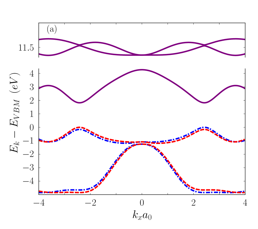
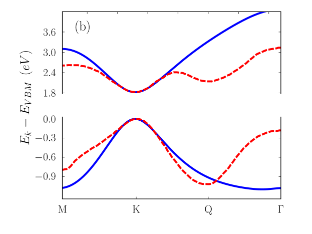
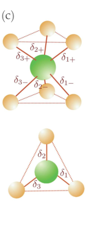
Figure 1: (Color online) (a) Band structure of ML-MDS consisting of five bands in which two are spin split in the valence band. The dot-dashed line refers to one spin and the dashed line denotes another spin component. Solid lines refer to the spin degenerate band. (b) A comparison between the band structure calculated by the present theory (solid lines) and the results calculated in Ref. [walle12, ] (dashed lines) based on density functional theory. Notice that our theory works quite well around the ${\bm{K}}$ point for the particle (hole or electron) density less than $10^{14}$cm^-2 ($E_{F}-E_{CBM}\simeq 0.2$ eV). Here, $a_{0}=a\cos\theta$ where $a$ is the length of Mo-S bond and $\theta$ is the angle between the bond and the $xy$ plane. (c) Side and top views of the lattice structure are seen where Mo atom (larger green sphere) is surrounded by six S atoms.

The Hamiltonian differs from that introduced by Xiao et al. xiao12 because of the second order terms in $q$. The diagonal $q^{2}$ terms, which contribute in the energy, to the same way as does the first order off-diagonal term, are responsible for the difference between electron and hole masses recently reported by using ab initio calculations walle12 . Moreover, the last term leads to anisotropic $q^{3}$ corrections to the energy which contribute to the trigonal warping effect. Importantly, $\alpha$ vanishes for the case that $m_{e}=-m_{h}$, however $\beta$ remains a constant. Basically, there is the possibility to have a cubic off-diagonal term in the low-energy Hamiltonian which in the calculation of the eigenvalues of the Hamiltonian are multiplied with the off-diagonal $q$ terms and eventually contributes at the same order as the diagonal $q^{2}$ terms. Since that term is very small, we thus ignore the $q^{3}$ off-diagonal term.

III Numerical results and Discussions

In this section, we present our main calculations for the electronic properties of MoS₂ by evaluating Eqs. (2), (3) and (4). We propose first the lattice Hamiltonian by considering numerical values of the hopping integrals and show the band structure of ML-MDS. Second, we present our numerical results for the electronic structure in two different models by exploring the Landau levels (LLs) and investigating the tunability of the electronic structure via an external perpendicular gate voltage.

Figure 1 shows the band structure of ML-MDS consisting of five bands for each spin in the absence of an external field. Two of them are spin polarized (dot-dashed and dashed lines) and the others are spin degenerate (solid lines). We note that due to the limitations of our model, the high energy bands may not be comparable with those of first principal calculations in a quantitative manner. Figure 1(b) shows a comparison between our results and those calculated by density functional theory walle12 indicating that our theory is in good agreement with density functional theory results close to the ${\bm{K}}$ point up to a high particle (hole or electron) density $10^{14}$cm^-2 (the Fermi energy is $E_{F}-E_{\rm CBM}\simeq 0.2$ eV). Nevertheless our effective model Hamiltonian does not provide a good description of the physics around the $\Gamma$ point where other orbitals like $p_{z}$ must be considered in order to describe the electronic dispersion Cappelluti13 .

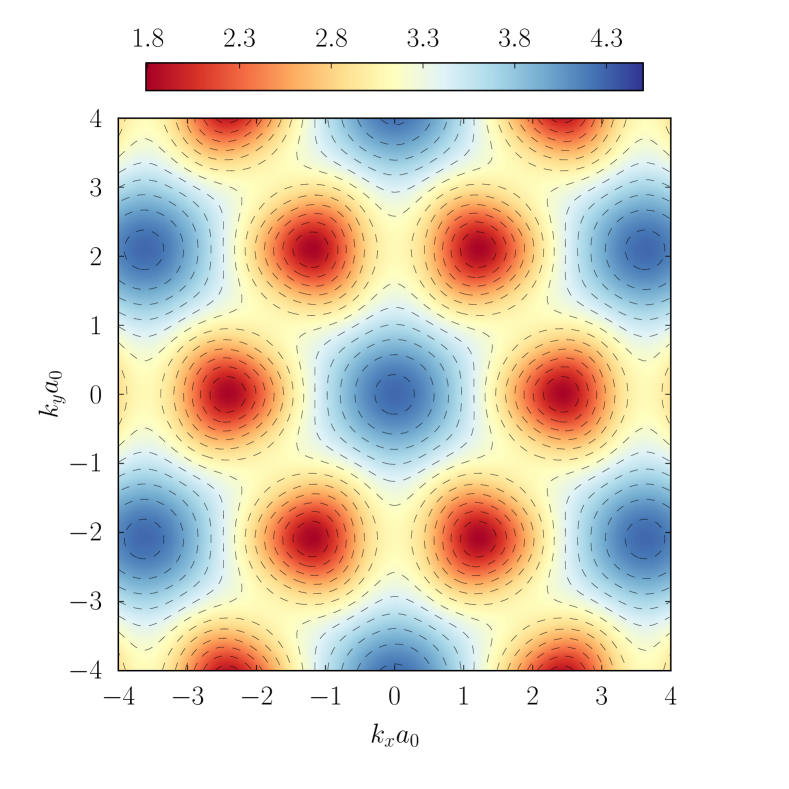
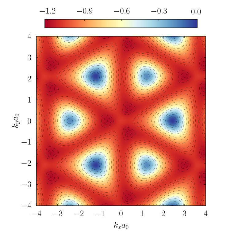
Figure 2: (Color online) Contour plots of the conduction (top panel) and valence (bottom panel) bands in momentum space for spin-up component together with isoenergy lines for to guide the eye. While the conduction band shows almost isotropic dispersion, the trigonal warping occurs in the valence band around $K$ points due to the difference of the orbital structures of the conduction and valance bands.

We further investigate the band structure close to the valence and conduction bands and our numerical results are shown, via contour plots which show the isoenergy lines, in Fig. 2. A strong anisotropy of the constant energy lines can be seen around $K$ points in the valence band, due to the trigonal warping, while in the conduction band all lines are almost isotropic; the warping is due to the difference of the orbital structure of the conduction and valence bands.

To study the interplay of spin and valley physics, we introduce, by ignoring trigonal warping, the effect of a time reversal symmetry breaking term by applying a perpendicular magnetic field, leading to the appearance of LLs as follows,

$$E^{\pm}_{n,\tau s} = \pm\sqrt{[\frac{\Delta-\lambda\tau s}{2}+\hbar\omega_{c}(\beta n-\frac{\alpha\tau}{2})]^{2}+2(\frac{t_{0}a_{0}}{l_{B}})^{2}n}$$ (5)

$$+\frac{\lambda\tau s}{2}+\hbar\omega_{c}(\alpha n-\frac{\beta\tau}{2}),~{}~{}~{}n=0,1,\dots$$

where $\omega_{c}=eB/2m_{0}$ and $l_{B}=\sqrt{\hbar/(eB)}$ are the cyclotron frequency and magnetic length, respectively. It should be noticed that the trigonal warping term, $t_{1}$, leads to a second order perturbation correction in the Landau level energy and accordingly its effect on the Landau levels is very weak. In contrast to Ref. niu12, , we see an additional valley degeneracy breaking term which is the reminiscent of the Zeeman-like coupling for valleys. As a result, the conduction band LLs are valley polarized and the valence band LLs are both valley and spin polarized although we have not yet considered the usual Zeeman interaction for spins. In particular, the $n=0$ LLs, $E^{+}_{0,\tau s}=[\Delta-\hbar\omega_{c}\tau(\beta+\alpha)]/2$ and $E^{-}_{0,\tau s}=\lambda\tau s-[\Delta+\hbar\omega_{c}\tau(\beta-\alpha)]/2$, depend on the magnetic field strength in opposite ways for the two valleys. More intriguingly, the splittings of LLs in the conduction and valence bands $\delta E^{+}\approx 5.4\hbar\omega_{c}$ and $\delta E^{-}\approx 4.6\hbar\omega_{c}$, differ from each other due to the difference of $m_{e}$ and $-m_{h}$. Furthermore, we can define extra splitting terms for LLs in the conduction and valence bands: valley splitting $\delta E^{+}_{v}=E^{+}_{-,s}-E^{+}_{+,s}=g_{v}^{+}\hbar\omega_{c}$ and spin splitting $\delta E^{+}_{s}=E^{+}_{\tau,-}-E^{+}_{\tau,+}=g_{s}\hbar\omega_{c}$ in the conduction band, and spin-valley splitting $\delta E^{-}_{s-v}=E^{-}_{-,\bar{s}}-E^{-}_{+,s}=(sg_{s}+g_{v}^{-})\hbar\omega_{c}$ in the valence band, with $g_{s}=2$, $g_{v}^{+}\approx\beta+\alpha$ ($g_{v}^{-}\approx\beta-\alpha$) indicating spin and valley g-factors for the conduction and valence bands. The splittings present in the conduction band, originate from the valley and spin contributions, separately, but the splitting in the valence band comes from both spin and valley terms. Notice that the valley splitting depends slightly on the amount of mixing with $p-$ orbitals for the conduction band through the parameter $\beta$ and the influence of the mixing value is very weak (see Appendix B for more details).

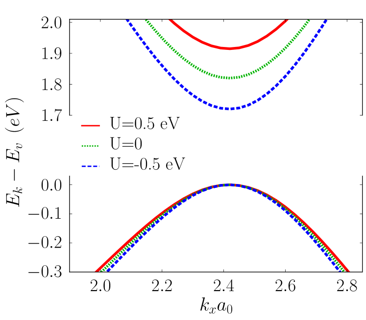
Figure 3: (Color online) Spin-up conduction and valence energy bands, referred to the energy $E_{v}=E_{VBM}+U/2$, for different values of the vertical bias.

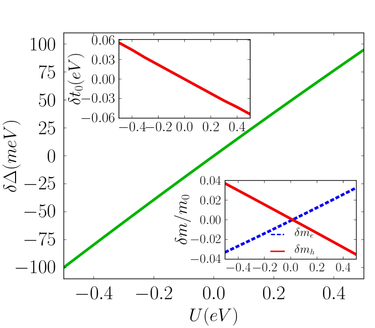
Figure 4: (Color online) Variation of the gap versus induced potential which is almost linear in the chosen range of $U$. Insets show the change in the effective hopping integral and the effective masses with $U$. Using the form of $U$-dependence of the parameters, we can also estimate the linear change of $\delta\alpha\approx-0.15U/$eV and $\delta\beta\approx-1.95U/$eV.

It is also important to investigate the tunability of the electronic structure via a perpendicular external electric field. The vertical bias breaks the mirror symmetry $\sigma_{h}$ and modifies the on-site energies of atoms in three sublayers of ML-MDS. Accordingly, these changes affect the whole electronic structure especially the low-energy characteristics such as $\Delta$, $m_{e}$, $m_{h}$ and the effective hopping $t_{0}$. Interestingly enough, the valley degeneracy breaking can be controlled by tuning $\alpha$ and $\beta$ due to the perpendicular gate voltage when the system is subjected to a perpendicular magnetic field. We assume a single-gated device in which the induced potentials take the values $U^{b}=0$ and $U^{b^{\prime}}=2U^{a}$. The variation of the mentioned parameters with the induced potential $U^{b^{\prime}}$ are shown in Figs. 3 and 4, where we illustrate only the low-energy band structure for different $U^{b^{\prime}}$ values. Using simple electrostatic arguments, the induced potentials for an applied vertical bias $V_{g}$ can be estimated as $U^{b^{\prime}}=\gamma eV_{g}$ with $\gamma\approx(d/L)\epsilon^{\prime}/\epsilon$ where $\epsilon$, $d$ and $\epsilon^{\prime}$, $L$ indicate the dielectric constants and thicknesses of ML-MDS and the substrate, respectively. For typical values $\epsilon\approx 6$ zhang02 , $\epsilon^{\prime}\approx 3.9$, $d\approx 0.32$ nm, and $L\approx 300$ nm with SiO₂ as the dielectric substrate, we obtain $\gamma\approx 0.0007$. By replacing the substrate with high-$\epsilon$ gate dielectrics like HfO₂ with $\epsilon^{\prime}\approx 25$ wallace , the coefficient $\gamma\approx 0.004$ increases and leads to $U^{b^{\prime}}\approx 0.4$eV for $V_{g}=100$V which is already used in the on-going experiments. Consequently, the perpendicular gate voltage effects are enhanced by using a proper substrate with large dielectric constant.

IV conclusion

In summary, we have formulated a tight-binding Hamiltonian in order to describe the low-energy band structure of monolayer MoS₂ which can be useful to study energy dispersion and transport phenomena in nanostructured MoS₂. We have obtained a seven-band model (for each spin component) in which four of them are contributed mainly from sulfur (S) $p$ orbitals and three remaining mostly originate from molybdenum (Mo) $d$ hybrids. Our model not only describes the low-energy behavior of monolayer MoS₂ which differs from massive Dirac fermion picture, but also predicts the difference between the effective hole and electron masses and the trigonal warping effect. In addition, the two-band model leads to a valley degeneracy breaking effect in the Landau levels and we have shown that the conduction band Landau levels are valley polarized and the valence band Landau levels are both valley and spin polarized. Finally, we have shown that by applying a perpendicular electric field to the monolayer the electronic structure especially the band gap and effective electron and hole masses can be finely tuned. It should be noted that our model is appropriate mostly for low-energy calculations in the vicinity of the conduction and valence bands.

Finally, we would like to emphasize that the diagonal quadratic terms in the low-energy Hamiltonian play an essential role in the transport and optical properties of the system Rostami133 . It is worth noting that the sign of the $\beta$ term can influence topological features of the system such as the Berry curvature, the valley Chern number which is defined as ${\cal C}_{v}\propto{\rm sign}(\Delta)-{\rm sign}(\beta)$, and $Z_{2}$ invariant which vanishes for $\beta\Delta>0$.

Note added– Recently, a paper Kormanyos13 which covers closely related material, has been published.

Appendix A Seven-band Hamiltonian

We start constructing an effective tight-binding model for the monolayer MoS₂ system, assuming the following basis orbitals,

$$|1\rangle = d_{z^{2}},$$

$$|2\rangle = \frac{1}{\sqrt{2}}(|d_{x^{2}-y^{2}}\rangle+i|d_{xy}\rangle),~{}~{}~{}|1^{\prime}\rangle=\frac{1}{\sqrt{2}}(|p_{x}\rangle+i|p_{y}\rangle),$$

$$|3\rangle = \frac{1}{\sqrt{2}}(|d_{x^{2}-y^{2}}\rangle-i|d_{xy}\rangle),~{}~{}~{}|2^{\prime}\rangle=\frac{1}{\sqrt{2}}(|p_{x}\rangle-i|p_{y}\rangle).$$

The Wannier functions for different lattice sites in a crystal are localized and they can be written as $|c,i,\mu\rangle=c^{\dagger}_{i\mu}|0\rangle$ where $i$ denotes the site and $\mu$ indicates atomic orbital. $c=a$ or $(b,b^{\prime})$ shows the annihilation operator of three different sublattices of monolayer MoS₂, consisting of one Mo and two S atoms. Up to the nearest-neighbor hopping integral, the tight binding Hamiltonian can be written as Eq. (1) in the main text,

$$\epsilon_{\mu\nu}^{c} = \langle c,i,\mu|H|c,i,\nu\rangle,$$

$$t_{ij,\mu\nu} = \langle a,i,\mu|H|b(b^{\prime}),j,\nu\rangle,$$ (6)

$$s_{ij,\mu\nu} = \langle a,i,\mu|b(b^{\prime}),j,\nu\rangle.$$

The lattice has two important symmetries $C_{3}=e^{-i\omega L_{z}/\hbar}$ and $\sigma_{v}:\{(x,y,z)\rightarrow(-x,y,z)\}$ where the first one is the trigonal rotational symmetry where $\omega=2\pi/3$ and $L_{z}$ is the $z-$component of orbital angular momentum and the second one indicates the reflection symmetry with respect to the $y-z$ plane. The action of these symmetry operators on the basis functions can be summarized in the following equations:

$$C {}_{3}|1\rangle=|1\rangle~{},~{}~{}~{}~{}~{}~{}~{}~{}~{}~{}~{}C_{3}\{|2\rangle,|2^{\prime}\rangle\}=e^{i\omega}\{|2\rangle,|2^{\prime}\rangle\}$$ (7)

$$C {}_{3}\{|3\rangle,|1^{\prime}\rangle\}=e^{-i\omega}\{|3\rangle,|1^{\prime}\rangle\},$$

$$\sigma {}_{v}\{|1\rangle,|2\rangle,|3\rangle\}=\{|1\rangle,|3\rangle,|2\rangle\}$$

$$\sigma {}_{v}\{|1^{\prime}\rangle,|2^{\prime}\rangle\}=-\{|2^{\prime}\rangle,|1^{\prime}\rangle\}.$$

It should be noticed that, here, we have dropped the spin indices. The symmetry relations in Eq. (7), impose some constraints on the on-site energies and hopping integrals, and thus we have

$$\epsilon^{a}=\begin{pmatrix}A_{1}&0&0\\ 0&A_{2}&0\\ 0&0&A_{2}\end{pmatrix}\,,~{}~{}~{}~{}~{}~{}\epsilon^{b}=\epsilon^{b^{\prime}}=\begin{pmatrix}B&0\\ 0&B\end{pmatrix}\,,$$

$$t_{\delta_{1\pm}}=\begin{pmatrix}t_{11}&-e^{-i\omega}t_{11}\\ t_{21}&t_{22}\\ -t_{22}&-e^{i\omega}t_{21}\end{pmatrix},~{}~{}t_{\delta_{2\pm}}=\begin{pmatrix}e^{i\omega}t_{11}&-e^{i\omega}t_{11}\\ e^{-i\omega}t_{21}&t_{22}\\ -t_{22}&-e^{-i\omega}t_{21}\end{pmatrix}$$

$$t_{\delta_{3\pm}}=\begin{pmatrix}e^{-i\omega}t_{11}&-t_{11}\\ e^{i\omega}t_{21}&t_{22}\\ -t_{22}&-t_{21}\end{pmatrix}.$$ (8)

Note that the same relations can be found for $s_{\delta_{i\pm}}$ by substituting the $t_{\mu\nu}$’s with $s_{\mu\nu}$’s. In the presence of spin-orbit interaction of the Mo atoms, it is easy to generalize $\epsilon^{a}$ by replacing $(\epsilon^{a})_{22}\rightarrow A_{2}+\lambda s$ and $(\epsilon^{a})_{33}\rightarrow A_{2}-\lambda s$. The subindices of the hopping matrices indicate the nearest-neighbor vectors,

$$\delta_{1\pm} = a(\frac{\sqrt{3}}{2}\cos\theta,-\frac{1}{2}\cos\theta,\pm\sin\theta),$$

$$\delta_{2\pm} = a(0,\cos\theta,\pm\sin\theta),$$ (9)

$$\delta_{3\pm} = a(\frac{-\sqrt{3}}{2}\cos\theta,-\frac{1}{2}\cos\theta,\pm\sin\theta),$$

where $a=2.43{\AA}$ and $\theta=40.7$ degree Yue12 are the Mo-S bond length and the angle between the bond and Mo’s plane, respectively. To find above equations, we also used the operation of $C_{3}$ and $\sigma_{v}$ on $\delta_{i\pm}$ as $C_{3}\delta_{1\pm}=\delta_{2\pm}$, $C_{3}\delta_{2\pm}=\delta_{3\pm}$, $\sigma_{v}\delta_{1\pm}=\delta_{3\pm}$ and $\sigma_{v}\delta_{2\pm}=\delta_{2\pm}$.

Following a method proposed by the Slater and Koster slater54 (SK), all hopping and overlap integrals can be written as linear combinations of $V_{pd\sigma}$ and $V_{pd\pi}$ and $S_{pd\sigma}$ and $S_{pd\pi}$. In this method, we define some standard hopping and overlap parameters as $V_{ll^{\prime}|m|}=\langle\vec{R}^{\prime},l^{\prime},m|H|\vec{R},l,m\rangle$ and $S_{ll^{\prime}|m|}=\langle\vec{R}^{\prime},l^{\prime},m|\vec{R},l,m\rangle$ where $m=0,1$ stands for $\sigma,\pi$ bonds and the other hopping and overlap integrals can be found from the SK table slater54 . In this way we find

$$t_{11} = -\frac{1}{\sqrt{2}}(n_{x}+in_{y})[\sqrt{3}n_{z}^{2}V_{pd\pi}+\frac{1}{2}(1-3n_{z}^{2})V_{pd\sigma}],$$

$$t_{21} = \frac{1}{2}(n_{x}-in_{y})[\frac{\sqrt{3}}{2}V_{pd\sigma}(1-n_{z}^{2})+V_{pd\pi}(1+n_{z}^{2})],$$

$$t_{22} = \frac{1}{2}(n_{x}-in_{y})^{3}(\frac{\sqrt{3}}{2}V_{pd\sigma}-V_{pd\pi}),$$ (10)

where ${\bf n}=(n_{x},n_{y},n_{z})$ is a unit vector pointing between the nearest-neighbor lattice points. Once again, we can obtain similar relations for the overlaps by substituting the hopping matrix elements with those of overlap matrix. These relations help us to reduce the number of independent hopping parameters from three to two. In the absence of external bias, due to the symmetry between the two sulfur sublattices, we can simply reduce the $7\times 7$ Hamiltonian to $5\times 5$ as below

$$\cal{H}=\begin{pmatrix}{\hat{H}}_{a}&2{\hat{H}}_{t}\\ 2{{\hat{H}}_{t}}^{\dagger}&2{\hat{H}}_{b}\end{pmatrix},~{}~{}~{}~{}~{}\cal{S}=\begin{pmatrix}1&2{\hat{S}}\\ {2{\hat{S}}}^{\dagger}&2\end{pmatrix}.$$ (11)

To find the unknown parameters, we should first obtain the energy bands around the $K$-point. After solving the generalized eigenvalue problem as $\cal H|\psi\rangle=\textit{E}\cal S|\psi\rangle$ at the $K$-point, we can find the energies as

$$E_{1} = A_{+},$$

$$E_{2} = \frac{(A_{1}+B)/2-18\Re e(t_{11}s_{11}^{*})-\sqrt{[(A_{1}+B)/2-18\Re e(t_{11}s_{11}^{*})]^{2}+(1-18|s_{11}|^{2})(18|t_{11}|^{2}-A_{1}B)}}{1-18|s_{11}|^{2}},$$

$$E_{3} = \frac{(A_{-}+B)/2-18\Re e(t_{21}s_{21}^{*})-\sqrt{[(A_{-}+B)/2-18\Re e(t_{21}s_{21}^{*})]^{2}+(1-18|s_{21}|^{2})(18|t_{21}|^{2}-A_{-}B)}}{1-18|s_{21}|^{2}},$$ (12)

$$E_{4} = \frac{(A_{1}+B)/2-18\Re e(t_{11}s_{11}^{*})+\sqrt{[(A_{1}+B)/2-18\Re e(t_{11}s_{11}^{*})]^{2}+(1-18|s_{11}|^{2})(18|t_{11}|^{2}-A_{1}B)}}{1-18|s_{11}|^{2}},$$

$$E_{5} = \frac{(A_{-}+B)/2-18\Re e(t_{21}s_{21}^{*})+\sqrt{[(A_{-}+B)/2-18\Re e(t_{21}s_{21}^{*})]^{2}+(1-18|s_{21}|^{2})(18|t_{21}|^{2}-A_{-}B)}}{1-18|s_{21}|^{2}}.$$

These eigenvalues include bonding (with lower energy) and anti-bounding ( with higher energy) of $p-d$ bands. Since the conduction and valence bands are mostly formed from $d_{z^{2}}$ and $d_{x^{2}-y^{2}}+id_{xy}$ orbital of Mo, therefore, $E_{1}$ and $E_{2}$ are the valence band maximum and the conduction band minimum located at the $K$-point, respectively.

Appendix B Two-band Hamiltonian

Here, we find the low-energy two-band effective Hamiltonian with the Löwdin partitioning method winkler . As described in the text, we change the nonorthogonal basis to an orthogonal one and then rotate them by using a unitary transformation, $U_{0}$, which diagonalize $\widetilde{H}_{0}$ so that we arrive as a new Hamiltonian,

$$H=U^{\dagger}_{0}{\cal S}^{-1/2}{\cal H}{\cal S}^{-1/2}U_{0},$$ (13)

where ${\cal H}={\cal H}_{0}+{\cal H}_{1}$ and up to the second order in $q=q_{x}+iq_{y}$, ${\cal H}_{1}$ is given by

$${\cal H}_{1}=\begin{pmatrix}0&0&0&-\frac{3}{2}e^{i\omega}t_{11}|q|^{2}a^{2}_{0}&-3e^{i\omega}t_{11}qa_{0}\\ 0&0&0&3e^{i\omega}t_{21}qa_{0}&-3t_{22}q^{*}a_{0}\\ 0&0&0&3t_{22}q^{*}a_{0}&-\frac{3}{2}e^{-i\omega}t_{21}|q|^{2}a^{2}_{0}\\ -\frac{3}{2}e^{-i\omega}t_{11}^{*}|q|^{2}a^{2}_{0}&3e^{-i\omega}t_{21}^{*}q^{*}a_{0}&3{t_{22}}^{*}qa_{0}&0&0\\ -3e^{-i\omega}{t_{11}}^{*}q^{*}a_{0}&-3{t_{22}}^{*}qa_{0}&-\frac{3}{2}e^{i\omega}{t_{21}}^{*}|q|^{2}a^{2}_{0}&0&0\end{pmatrix},$$ (14)

where $a_{0}=a\cos\theta$. In order to find the unitary transformation matrix, the eigenvectors of $\widetilde{H}_{0}={S_{0}}^{-1/2}{\cal H}_{0}{S_{0}}^{-1/2}$ are obtained first. Fortunately, ${\cal S}_{0}^{-1/2}$ can be analytically calculated at the $K$ point, however, for nonzero values of $q$, an iterative method Denman76 should be used. Therefore, in the vicinity of the $K$-point, we can treat ${\cal H}_{1}$ as a perturbation by assuming small enough $q$ values and the transformed Hamiltonian, $H$, can be expressed as the sum of two parts where $V$ is a perturbation term,

$$H_{\rm diag}=\begin{pmatrix}h_{11}[2\times 2]&0\\ 0&h_{22}[3\times 3]\end{pmatrix},$$

$$V=\begin{pmatrix}0&h_{12}[2\times 3]\\ {h_{12}}^{\dagger}[3\times 2]&0\end{pmatrix}.$$ (15)

Now, we can employ the quasi-degenerate perturbation theory that is based on the idea of constructing a unitary operator $e^{-\cal O}$ in such a way to drop the first-order $V$ in the transformed Hamiltonian, $H^{\prime}=e^{-\cal O}H{e^{\cal O}}=H_{\rm diag}+V+[H_{\rm diag},{\cal O}]+[V,{\cal O}]+\frac{1}{2}[[H_{\rm diag},{\cal O}],{\cal O}]+\cdots$. This imposes the constraint $V+[H_{diag},{\cal O}]=0$ which leads to the following form for the generator of the transformation,

$${\cal O}=\begin{pmatrix}0&\eta[2\times 3]\\ -\eta^{\dagger}[3\times 2]&0\end{pmatrix},$$ (16)

with the property that $\eta h_{22}-h_{11}\eta=h_{12}$. Then $H^{\prime}=H_{\rm diag}+\frac{1}{2}[V,{\cal O}]+\cdots$ is an effective Hamiltonian with two decoupled subspaces. Following straightforward calculations, the effective Hamiltonian of the low-energy bands can be obtained as follows

$$h_{11}-\frac{1}{2}\{\eta{h_{12}}^{\dagger}+h_{12}\eta^{\dagger}\}.$$ (17)

Insertion of matrix form of operators $h_{11}$, $h_{12}$, and $\eta$ results in the two-band form proposed in Eq. (4) in the text as

$$H_{\tau s} = \frac{\Delta}{2}\sigma_{z}+\lambda\tau s\frac{1-\sigma_{z}}{2}+t_{0}a_{0}{\bf q}\cdot{\bm{\sigma}}_{\tau}$$ (18)

$$+ \frac{\hbar^{2}|{\bf q}|^{2}}{4m_{0}}(\alpha+\beta\sigma_{z})+t_{1}a_{0}^{2}{\bf q}\cdot{\bm{\sigma}}^{\ast}_{\tau}\sigma_{x}{\bf q}\cdot{\bm{\sigma}}^{\ast}_{\tau}$$

for spin $s=\pm$ and valley $\tau=\pm$.

It should be noticed that the parameters of the tight-binding model dependence on the $p-$orbital mixing do not have a simple form which prevents us from introducing an analytical relation between the parameters of the two-band model Hamiltonian and the $p-$orbital percentage. The parameter $\alpha$ depends only on the effective mass difference between the conduction and valence bands. The energy gap and the spin orbit splitting do not depend on the mixing. Therefore, the influence of the mixing parameter has been checked for $5\%$ and $15\%$ mixing and they lead to the following values $\beta=2.30$ and $2.15$, $t_{0}=1.65$ and $1.70$, respectively. In addition, the values of the effective hopping trigonal wrapping $t_{1}$ in the low-energy Hamiltonian change slightly with variation in the mixing value by $1\%$ which can be neglected.

References

• (1) K. S. Novoselov, A. K. Geim, S. V. Morozov, D. Jiang, Y. Zhang, S. V. Dubonos, I. V. Grigorieva, A. A. Firsov, Science 306, 666 (2004).
• (2) K. F. Mak, C. Lee, J. Hone, J. Shan, and T. F. Heinz, Phys. Rev. Lett. 105, 136805 (2010); A. Splendiani, L. Sun, Y. Zhang, T. Li, J. Kim, C. Y. Chim, G. Galli, and F. Wang, Nano Lett. 10, 1271 (2010); T. Korn, D. Stich, R. Schulz, D. Schuh, W. Wegscheider, and C. Schüller, Appl. Phys. Lett. 99, 102109 (2011).
• (3) B. Radisavljevic, A. Radenovic, J. Brivio, V. Giacometti and A. Kis, Nature Nanotech. 6, 147 (2011).
• (4) D. Xiao, D. Xiao, G. Liu, W. Feng, X. Xu, and W. Yao, Phys. Rev. Lett. 108, 196802 (2012).
• (5) H. Zeng, J. Dai, W. Yao, D. Xiao, and X.D. Cui, Nature Nanotech. 7, 490 (2012).
• (6) T. Cao, G. Wang, W. Han, H. Ye, C. Zhu, J. Shi, Q. Niu, P. Tan, E. Wang, B. Liu, and J. Feng, Nature Commun. 3, 887 (2012).
• (7) Q. H. Wang, K. Kalantar-Zadeh, A. Kis, J. N. Coleman and M. S. Strano, Nature Nanotech. 7, 699 (2012).
• (8) G. Sallen, L. Bouet, X. Marie, G. Wang, C. R. Zhu, W. P. Han, Y. Lu, P. H. Tan, T. Amand, B. L. Liu, and B. Urbaszek, Phys. Rev. B 86, 081301(R) (2012).
• (9) K. F. Mak, K. He, J. Shan, and T. F. Heinz, Nature Nanotech. 7, 494 (2012); K. F. Mak, K. He, C. Lee, G. Hyoung Lee, J. Hone, Tony F. Heinz, and J. Shan, Nature Mat. 12, 207 (2013);
• (10) S. Wu, J.S. Ross, Gui-Bin Liu, G. Aivazian, A. Jones, Z. Fei, W. Zhu, D. Xiao, W. Yao, D. Cobden and X. Xu Nature Physics 9, 149 (2013); K. Behnia, Nature Nanotech. 7, 488 (2012).
• (11) R. A. Bromley, R. B. Murray, and A. D. Yoffe, J. Phys. C 5, 759 (1972).
• (12) L. F. Mattheiss, Phys. Rev. B 8, 3719 (1973); D. W. Bullett, J. Phys. C 11, 4501 (1978).
• (13) E. S. Kadantsev, P. Hawrylak, Solid State Commun. 152, 909 (2012); H. Shi, H. Pan, Y.-W. Zhang, B. I. Yakobson, Phys. Rev. B 87, 155304 (2013).
• (14) J. Kang, J. Kang, S. Tongay, J. Li and J. Wu, Appl. Phys. Lett. 102, 012111 (2013).
• (15) J. K. Ellis, M. J. Lucero, and G. E. Scuseria, Appl. Phys. Lett. 99, 261908 (2011); C. Ataca, H. Şahin and, S. Ciraci, J. Phys. Chem. C 116, 8983 (2012); S. Lebègue and O. Eriksson, Phys. Rev. B 79, 115409 (2009); Z. Y. Zhu, Y. C. Cheng, and U. Schwingenschlögl, ibid 84, 153402 (2011); D. Le, D. Sun, W. Lu, L. Bartels, and T. S. Rahman, ibid 85, 075429 (2012); T. Cheiwchanchamnangij and W. R. L. Lambrecht, ibid 85, 205302 (2012); A. Ramasubramaniam, ibid 86, 115409 (2012).
• (16) X. Li, F. Zhang, and Q. Niu, Phys. Rev. Lett. 110, 066803 (2013).
• (17) J. C. Slater and G. F. Koster, Phys. Rev. 94, 1498 (1954).
• (18) E. Cappelluti, R. Roldán, J.A. Silva-Guillén, P. Ordejón, F. Guinea, arXiv:1304.4831(2013).
• (19) H. Peelaers and C. G. Van de Walle, Phys. Rev. B 86, 241401(R) (2012).
• (20) Y. Li, Y.-L. Li, C. Moyses Araujo, W. Luo, and R. Ahuja, arXiv:1211.4052 (2012).
• (21) R. Winkler, Spin Orbit Coupling Effects in Two-Dimensional Electron and Hole Systems (Springer, Berlin, 2003).
• (22) X. Zhang, D. O. Hayward, and D. M. P. Mingos, Catalyst Lett. 84, 225 (2002).
• (23) G. D. Wilka, R. M. Wallaceb, Appl. Phys. Rev. 89, 5243 (2001).
• (24) Q. Yue, J. Kang, Z. Shao, X. Zhang, S. Chang, G. Wang, S. Qin, and J. Li, Phys. Lett. A 376, 1166 (2012).
• (25) E. D. Denman, A. N. Beavers, Applied Mathematics and Computation 2, 63 (1976).
• (26) H. Rostami and R. Asgari (unpublished).
• (27) A. Kormanyos, V. Zolyomi, N. D. Drummond, P. Rakyta, G. Burkard, and V. I. Fal’ko, Phys. Rev. B 88, 045416 (2013).