A simple model of ultrasound propagation in a cavitating liquid. Part II: Primary Bjerknes force and bubble structures.

Abstract

In a companion paper, a reduced model for propagation of acoustic waves in a cloud of inertial cavitation bubbles was proposed. The wave attenuation was calculated directly from the energy dissipated by a single bubble, the latter being estimated directly from the fully nonlinear radial dynamics. The use of this model in a mono-dimensional configuration has shown that the attenuation near the vibrating emitter was much higher than predictions obtained from linear theory, and that this strong attenuation creates a large traveling wave contribution, even for closed domain where standing waves are normally expected. In this paper, we show that, owing to the appearance of traveling waves, the primary Bjerknes force near the emitter becomes very large and tends to expel the bubbles up to a stagnation point. Two-dimensional axi-symmetric computations of the acoustic field created by a large area immersed sonotrode are also performed, and the paths of the bubbles in the resulting Bjerknes force field are sketched. Cone bubble structures are recovered and compare reasonably well to reported experimental results. The underlying mechanisms yielding such structures is examined, and it is found that the conical structure is generic and results from the appearance a sound velocity gradient along the transducer area. Finally, a more complex system, similar to an ultrasonic bath, in which the sound field results from the flexural vibrations of a thin plate, is also simulated. The calculated bubble paths reveal the appearance of other commonly observed structures in such configurations, such as streamers and flare structures.

1 Introduction

A common observation in acoustic cavitation experiments is the rapid translational motion of the bubbles relative to the liquid, and their self-organization into various spectacular structures. These structures have been systematically reviewed recently [1], and some of them have been successfully explained by results derived from single bubble physics [2, 1, 3].

The origin for bubble translational motion in an acoustic field is the so-called Bjerknes force [4, 5, 6], which is the average over one oscillation period of the generalized buoyancy force exerting on any body in an accelerating liquid [7]. It is commonly expressed in terms of the pressure gradient as:

$$\mathbf{F_{B}}=-\left<V\boldsymbol{\nabla}p\right>,$$ (1)

where $\left<.\right>$ denotes the average over one acoustic period, $V$ is the bubble volume and $p$ the acoustic pressure which would exist in the liquid at the center of the bubble if the latter were not present. Since $V$ and $p$ are oscillatory, the average of their product can be non-zero.

The most spectacular and known manifestation of the primary Bjerknes force occurs in standing waves. It can be simply deduced from linear theory that bubbles smaller than the resonant size are attracted by pressure antinodes, whereas bubbles larger than resonant size are attracted by pressure nodes [8]. This was confirmed by the early experiments of Crum & Eller [9], and is the basic principle of levitation experiments used to study single bubble sonoluminescence, where attraction by the central antinode of the flask counteracts the buoyancy force [10, 11].

However, nonlinear effects can produce repulsion of inertial bubbles from pressure antinodes above a given threshold [6]. This threshold can be estimated analytically for low frequency driving and is found to be near 170 kPa, with a slight dependence on surface tension [12]. This can be evidenced in multi-bubble experiments by a void region near the pressure antinode surrounded by bubbles accumulating near the threshold zone [2], or by bubbles self-arrangement into parallel layers shifted relative to the antinodal planes [1], correctly predicted by particle model simulations.

A more important issue concerns the Bjerknes force exerted on bubbles by large amplitude traveling waves. While small amplitude traveling waves exert a negligible Bjerknes force on bubbles, this is no longer true for large traveling waves, and theory predicts a large Bjerknes force, oriented in the direction of the wave propagation [13, 1, 3]. This means that an ultrasonic source emitting a traveling wave would strongly repel the bubbles nucleating on its surface. This issue has been investigated theoretically by Koch and co-workers [14], who, assuming an arbitrary wave, traveling in the sonotrode direction and standing in the perpendicular plane, showed that the conical bubble structure observed under large area transducers [15, 16] could be partially reproduced by particle models.

Other complex bubble structures can be observed in other configurations, such as ultrasonic baths, and were conjectured to result from a combination of both traveling and standing waves [1]. This raises the issue of the origin of such traveling waves, which was one of the motivation of the present paper and the companion one (which we will denote hereinafter by $[$OL I$]$). In the latter, we showed that traveling waves appear as a simple consequence of the attenuation by inertial bubbles. The model presented in $[$OL I$]$ constitutes therefore the missing link in the theory, and allows to calculate the acoustic field without any a priori on its structure, just from the knowledge of the vibrations of the ultrasonic emitter, whatever its complexity. From there, the Bjerknes force field can be calculated, and the shape of the structures formed by the bubble paths in the liquid can be examined.

Before going further, one should remind that Eq. (1) is an over-simplification of the complex problem of bubbles translational motion. A correct representation of the latter requires to write Newton’s second law for the bubble, accounting not only for the instantaneous driving force $-V\nabla p$ [of which (1) is the time-average], but also for viscous drag and added-mass forces [7]. All members of such an equation are dependent of the bubble radial dynamics, so that considering Eq. (1) as a mean force pushing the bubbles is a reduced view of the reality, masking the periodic translational motion superimposed to the (macroscopically visible) average translational motion. This is historically justified, since the first studies on Bjerknes forces aimed at localizing the stagnation points of the bubbles where $\mathbf{F_{B}}$ vanishes [17], as is the case in the center of single-bubble levitation experiments [10, 18]. Slightly extrapolating this point of view, if one accepts that the average bubble velocity can be obtained approximately by a balance between Eq. (1) and an average viscous drag force, a terminal mean velocity of the bubble can be calculated, which allowed for example successful particle simulations of bubble structures [2]. This raises the issue of nontrivial averaging procedure for moderate or large drivings [19, 20], which may be performed by elaborate multiple scales procedures [21]. However, some experimental situations exist where such a terminal velocity cannot be defined, and a bubble may wander between the nodes and antinodes of a standing wave [22]. The description of such a phenomenon requires the simultaneous resolution of the instantaneous radial and translational equations of the bubble, initially proposed in Ref. [23], and improved recently by a Lagrangian formulation [24, 25, 26]. The main result of the latter studies is that the radial and translational motions are strongly coupled, so that the bubble dynamics equation is also affected by the translational motion. Direct simulation of the two coupled equations in standing waves fields reveal that, apart from the classical scheme of bubble migration toward stagnation points, some bubbles may have no spatial attractors and can wander indefinitely between a node and an antinode, as observed in [22]. Such a behavior, termed as “translationally unstable”, has been found to result from an hysteretic response of the radial bubble dynamics below the main resonance [27].

In spite of the latter remarks, we will keep in this paper the classical picture of the mean primary Bjerknes force defined by Eq. (1) acting on the bubbles, and focus on the effects of traveling waves. The paper is organized as follows: in section 2, we will first briefly recall the main results on the primary Bjerknes force, and indicate how it can be calculated for an arbitrary bubble dynamics in a given acoustic field. In section 3, we will calculate the Bjerknes force field in acoustic fields calculated with the model proposed in $[$OL I$]$, which we will briefly recall in section 3.1. First, in section 3.2, the 1D configuration examined in $[$OL I$]$ will be considered. Then, in section 3.3, we will examine a 2D axi-symmetrical configuration, constituted by a large area sonotrode emitting in a large bath, similar to the experiments reported in Refs. [15, 16, 28]. Finally, section 3.4 will address another 2D configuration, mimicking an ultrasonic bath in which the acoustic field is produced by a plate undergoing flexural vibrations. For both 2D configurations, the bubble paths will be drawn from the knowledge of the acoustic and Bjerknes force fields at every point in the liquid. The structures obtained will be compared to experimental results of the literature and discussed.

2 Primary Bjerknes forces

2.1 Intuitive analysis and linear case

The physical origin of the primary Bjerknes force can be recalled simply by considering a mono-dimensional wave. The instantaneous pressure force exerted by the external liquid on a liquid sphere that would replace the bubble is approximately the difference $\Delta p$ between the instantaneous acoustic pressures on two opposite sizes of the sphere, multiplied by the bubble area $S$. Besides, the pressure difference $\Delta p$ is roughly $\partial p/\partial x\times 2R$, so that the instantaneous force is roughly $2R\times S\times\partial p/\partial x\simeq V\partial p/\partial x$. Generalizing this result in 3D Eq. (1) is recovered.

Along an acoustic cycle, the bubble therefore wanders forward and backward along the direction of the pressure gradient, under the influence of this instantaneous force, but the two motions may not exactly compensate, because the bubble may be for example larger when the pressure gradient is directed forward than when it is directed backward. The average force is therefore a matter of phase between the volume $V$ and the pressure gradient $\partial p/\partial x$, which can be better understood with the schematic representation of Fig. 1: the phase shift between $V$ and $\partial p/\partial x$ can be decomposed into two part: the phase shift $\gamma$ between volume $V$ and pressure $p$, and the phase shift $\theta$ between $p$ and its gradient $\partial p/\partial x$. The former depends on the way the bubble responds to the local acoustic field, that is on the bubble dynamics, whereas the latter depends on the structure of the acoustic field. All the results mentioned in the introduction can be interpreted from this picture.

Figure 1: Schematic interpretation of Eq. (1). The phase shift between bubble volume $V$ and pressure gradient $\partial p/\partial x$ can be decomposed into two parts: $\gamma$ depending on the bubble dynamics, and $\theta$ depending on the acoustic field.

Let’s take for example the case of sub-resonant bubble oscillating linearly. In this case, pressure and volume are in opposition ($\gamma=\pi$). In a pure 1D linear standing wave, away from pressure nodes or antinodes, $p$ and $\partial p/\partial x$ are either in phase ($\theta=0$), or in phase opposition ($\theta=\pi$), depending on the location relative to the pressure antinode. Thus, the phase shift between $V$ and $\partial p/\partial x$ is either $0$ or $\pi$. This yields therefore a large average value for the product $\left<V\partial p/\partial x\right>$, except in the pressure antinodes and nodes where it is zero. Conversely, for a traveling wave, pressure and pressure gradient are in quadrature ($\theta=\pi/2$), so that $\left<V\partial p/\partial x\right>$ is clearly zero in this case.

If the analysis is rather simple for linear oscillations, this is no longer the case for strongly nonlinear inertial oscillations. In that case, the bubble radial motion is mainly driven by the inertia of the liquid, and the bubble radius contains a large out-of-phase component with respect to the driving pressure $p$. This is the reason why pressure antinodes may become repulsive even for a sub-resonant bubble in a large amplitude standing wave [6], and why the Bjerknes force may become very large in traveling waves [13, 14]. The next section quantifies this qualitative analysis

2.2 General calculation of the Bjerknes force

The model described in $[$OL I$]$ was shown to result from the assumption that the bubbles mainly respond to the first harmonic of the field, which we termed as “first harmonic approximation” (FHA). We therefore assume that the pressure field in the liquid is mono-harmonic at angular frequency $\omega$, and defined in any point $\mathbf{r}$ by

$$p(\mathbf{r},t)=p_{0}+\frac{1}{2}\biggl{(}P(\mathbf{r})e^{i\omega t}+\overline{P}(\mathbf{r})e^{-i\omega t}\biggr{)},$$ (2)

which, writing $P=|P(\mathbf{r})|\exp\bigl{(}i\phi(\mathbf{r})\bigr{)}$, can be recast as

$$p(\mathbf{r},t)=p_{0}+|P(\mathbf{r})|\cos\left[\omega t+\phi(\mathbf{r})\right]$$ (3)

This expression may represent a traveling wave, a standing wave, or any combination of both. We also define the pressure gradient in general form as

$$\frac{\partial p}{\partial x_{i}}(\mathbf{r},t)=G_{i}(\mathbf{r})\cos\left[\omega t+\psi_{i}(\mathbf{r})\right],$$ (4)

where the fields $G_{i}$ and $\psi_{i}$ can be expressed as functions of $P$ and $\phi$ once the acoustic field is known.

The following two extreme cases deserve special consideration: for a standing wave, $\phi(\mathbf{r})=\phi_{0}$, so that $G_{i}(\mathbf{r})=\partial P/\partial x_{i}$ and $\psi_{i}(\mathbf{r})=\phi_{0}$; for a traveling wave, $P(\mathbf{r})=P_{0}$ and $\phi(\mathbf{r})=-\mathbf{k}.\mathbf{r}$ so that $G_{i}(\mathbf{r})=k_{i}P_{0}$ and $\psi_{i}(\mathbf{r})=\phi(\mathbf{r})-\pi/2$.

The expression of the Bjerknes force on the bubble located at $\mathbf{r}$ reads, from (1):

$$\mathbf{F_{B}}_{i}=-G_{i}(\mathbf{r})\frac{1}{T}\int_{0}^{T}V(\mathbf{r},t)\cos\left[\omega t+\psi_{i}(\mathbf{r})\right]\;dt,$$ (5)

where $T$ is the acoustic period and $V(\mathbf{r},t)$ is the instantaneous volume of a bubble located at $\mathbf{r}$ and can be calculated by solving a radial dynamics equation, for example:

$$\rho_{l}\left(R\ddot{R}+\frac{3}{2}\dot{R}^{2}\right)=p_{g}-\frac{2\sigma}{R}-4\mu_{l}\frac{\dot{R}}{R}-p(\mathbf{r},t).$$ (6)

The bubble volume depends on $\mathbf{r}$ because two bubbles located at different points may be excited by fields of different amplitudes $|P|$ but also different phases $\phi$. However, in order to be able to calculate the volume $V$ of any bubble over one acoustic period independently of its spatial location, we must fix the phase of the driving field in Eq. (6) by a convenient change of variables. We therefore set, taking this opportunity to non-dimensionalize the variables:

$$p(\mathbf{r},t)=p_{0}\left(1-|P^{*}|\cos\tau^{*}\right),$$ (7)

where the minus sign has been chosen to be consistent with earlier studies [29, 12], and, comparing this expression with Eq. (3), we get:

$$P^{*}=P(\mathbf{r})/p_{0},$$ (8)

$$\tau^{*}(\mathbf{r},t)=\omega t+\phi(\mathbf{r})-\pi.$$ (9)

We now note $V(\tau^{*})$ the volume of the bubble when it is driven by the pressure field (7), and making the change of variables in (5), we get:

$$\mathbf{F_{B}}_{i}=G_{i}(\mathbf{r})\frac{1}{2\pi}\int_{0}^{2\pi}V(\tau^{*})\cos\left[\tau^{*}-\phi(\mathbf{r})+\psi_{i}(\mathbf{r})\right]\;d\tau^{*},$$ (10)

which we recast as:

$$\mathbf{F_{B}}_{i} = G_{i}(\mathbf{r})\biggl{(}I_{C}\cos\left[\phi(\mathbf{r})-\psi_{i}(\mathbf{r})\right]$$

$$+I_{S}\sin\left[\phi(\mathbf{r})-\psi_{i}(\mathbf{r})\right]\biggr{)}.,$$ (11)

with

$$I_{C}=\frac{1}{2\pi}\int_{0}^{2\pi}V(\tau^{*})\cos\tau^{*}\;d\tau^{*},$$ (12)

$$I_{S}=\frac{1}{2\pi}\int_{0}^{2\pi}V(\tau^{*})\sin\tau^{*}\;d\tau^{*}.$$ (13)

This decomposition (which was suggested in a slightly different form by Mettin [1]), has the advantage to clearly decompose the respective influences of the bubble dynamics through integrals $I_{C}$ and $I_{S}$, and the one of the acoustic field, through the phase shift $\phi(\mathbf{r})-\psi_{i}(\mathbf{r})$. In the case of a 1D wave, the latter corresponds to the angle $\theta$ that we defined in figure 1. Integral $I_{C}$ measures the standing wave contribution to the Bjerknes force ($\phi-\psi=0$ or $\pi$), while integral $I_{S}$ measures the traveling wave contribution ($\phi-\psi=\pm\pi/2$).

The two integrals $I_{C}$ and $I_{S}$ can be easily calculated numerically by solving a radial dynamics equation to obtain $V$ and averaging over one period. They can also be calculated analytically, trivially for linear oscillations, and in a more complex manner for inertial oscillations in a small size range above the Blake threshold [12]. The correct matching between the two extreme cases is however difficult, so that we will use the numerical values hereinafter.

The results are displayed in Fig. 2 in the case of air bubbles in water in ambient conditions for two ambient radii $R_{0}=3$ $\mu$m (solid lines) and $R_{0}=5$ $\mu$m (dashed lines). The integral $I_{C}$ is represented in signed logarithmic scale (note the different scales for the positive and negative parts). It is seen that it is positive for low drivings, and quickly increases near the Blake threshold by about 3 orders of magnitude. In this range of acoustic pressures, antinodes are attractive. Then, above $|P^{*}|=1.7$ bar, $I_{c}$ becomes largely negative and the antinodes become repulsive, as was found in Ref. [6].

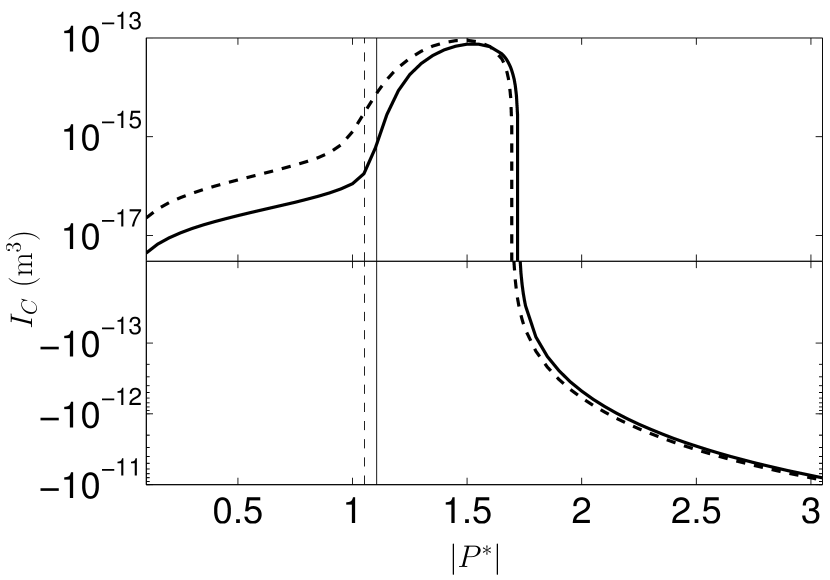
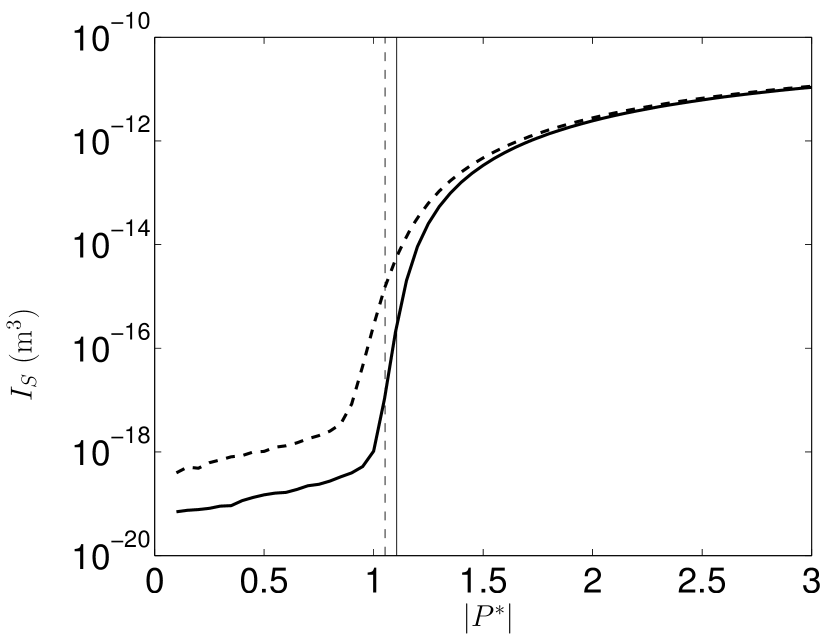
Figure 2: Average quantities $I_{C}$ and $I_{S}$ for an air bubble of ambient radius 3 $\mu$m (solid line) and 5 $\mu$m (dashed line) in water, as a function of the dimensionless acoustic pressure $|P^{*}|$ for frequency of 20 kHz. The vertical lines represent the Blake thresholds for 3 $\mu$m (solid) and 5 $\mu$m bubbles (dashed).

The integral $I_{S}$ is always positive, is very weak below the Blake threshold, and drastically increases above the Blake threshold (by 6 to 7 orders of magnitude). This predicts that, as reported in Ref. [13], the Bjerknes force can become very large in traveling waves.

3 Results

3.1 Simulation method

The complex acoustic field $P$ is obtained by solving a nonlinear Helmholtz equation, which has been detailed in $[$OL I$]$ and is briefly recalled here for completeness:

$$\nabla^{2}P+k^{2}\left(|P|\right)P=0.$$ (14)

where the complex wave number is given by:

$$\Re(k^{2})=\frac{\omega^{2}}{c_{l}^{2}}+\frac{4\pi R_{0}\omega^{2}N}{\omega_{0}^{2}-\omega^{2}},$$ (15)

$$\Im\left(k^{2}\right)=-2\rho_{l}\omega N\frac{\Pi_{\text{th}}+\Pi_{\text{v}}}{|P|^{2}}.$$ (16)

The bubble number $N$ is defined as a step function: it is assumed zero in the zones where the acoustic pressure is less than the Blake threshold, and is assigned to a constant value in the opposite case.

$$N=\left\{\begin{array}[]{lll}N_{0}&\text{if }|P|>P_{B}\\ 0&\text{if }|P|<P_{B}\end{array}\right.$$ (17)

3.2 1D results

We first calculate the primary Bjerknes force for the same 1D configuration as in $[$OL I$]$: the domain length is 10 cm, the right boundary is assumed infinitely soft, air bubbles of ambient radius 5 $\mu$m in water. For a low amplitude of the emitter ($U_{0}=0.3$ $\mu$m), the pressure amplitude profile is almost a perfect standing wave (Fig. 3a), and Fig. 3b exhibits the classical picture of a somewhat low primary Bjerknes force pushing the bubbles towards the antinodes (note that the distortion of the force profile in Fig. 3b is an artifact of the signed logarithmic scale used in ordinate). In this case, the value of the Bjerknes force mainly owes to the $I_{C}$ term in Eq. (11).

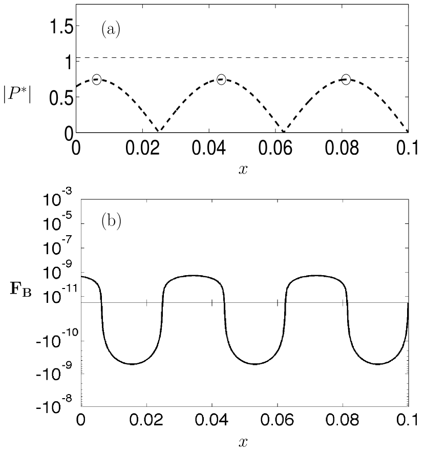
Figure 3: Simulation of the sound field and resulting primary Bjerknes force for 5 $\mu$m air bubbles in water, with an emitter displacement amplitude is $U_{0}$= 0.3 $\mu$m at 20 kHz. (a): Pressure amplitude profile. The horizontal dashed line represents the Blake threshold for 5 $\mu$m bubbles. (b): Bjerknes force exerted on bubbles at each point of the domain (with signed logarithmic scale in ordinate). The circles in Fig. (a) represents the stable stagnation points for the bubble.

For larger emitter amplitude ($U_{0}=5$ $\mu$m), the pressure amplitude profile is strongly damped near the emitter, as already commented in $[$OL I$]$ (Fig. 4a). This strong attenuation produces a noticeable traveling part in the wave and thus a large $I_{S}$ term in Eq. (11), which, as shown in Fig. 4b, results in a huge positive force near the emitter almost 6 orders of magnitude higher than the maximal force visible in Fig 3b (note that the scales used in both figures are identical). The bubbles would consequently be strongly expelled from the emitter, and travel right to the first stagnation point which is located somewhat far from the emitter (see the leftmost circle marker on Fig. 4a). The occurrence of such stagnation points has been proposed to be the key mechanism for bubble conical structure formation [14, 1]. We will show in the next section that this is partially true, but involves some additional subtleties.

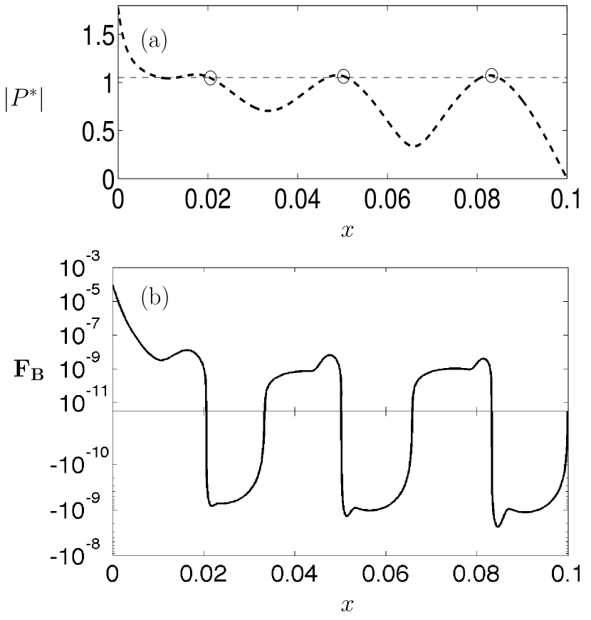
Figure 4: Simulation of the sound field and resulting primary Bjerknes force for 5 $\mu$m air bubbles in water, with an emitter displacement amplitude is $U_{0}$= 5 $\mu$m at 20 kHz. (a): Pressure amplitude profile. The horizontal dashed line represents the Blake threshold for 5 $\mu$m bubbles. (b): Bjerknes force exerted on bubbles at each point of the domain (with signed logarithmic scale in ordinate). The circles in Fig. (a) represents the stable stagnation points for the bubble.

3.3 Sonotrode

3.3.1 Experiments with a 12 cm diameter sonotrode

In this section we compare the results of our model to cone bubble structures images presented in Ref. [15]. The latter work used a 100 cm $\times$ 60 cm rectangular water tank of 40 cm depth, where a sonotrode of diameter $2a=$ 12 cm driven at 20.7 kHz is immersed at 3 cm below the free liquid level (Fig. 5).

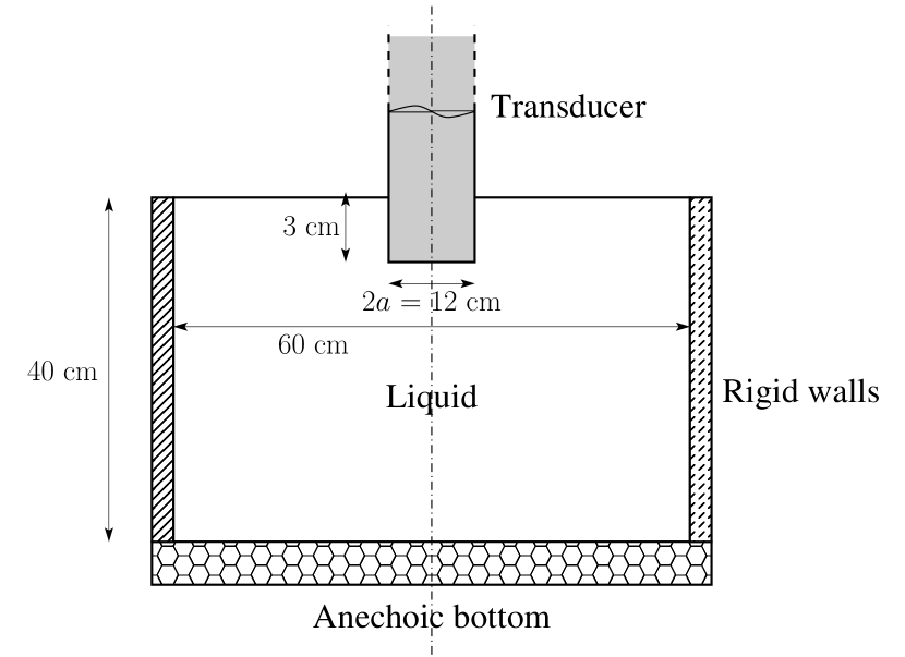
Figure 5: Axi-symmetrical geometry for large area sonotrode.

The geometry simulated follows the experimental configuration used in Ref. [15] as closely as possible. However, in order to avoid time-consuming 3D simulations, we replaced the rectangular tank by a cylindrical one with the same depth and a diameter of 60 cm, and simulate only a half-plane cut in axi-symmetrical mode. The characteristic of the bottom of the tank is not specified in Ref. [15] but following a similar work by the same authors in which the same bubble structures were observed [16], we considered an anechoic tank bottom. The lateral sides of the tank were taken as infinitely rigid boundaries, and the free liquid surface as infinitely soft. The nonlinear Helmholtz equation with the latter boundary conditions was solved in axi-symmetrical geometry, using the commercial COMSOL software.

The transducer is also simulated in order to account for its lateral deformation in the liquid, which, as will be seen below, is necessary to catch some experimental features. However, since details on the internal structure of the transducer are not given in Refs. [15, 16], we assumed the latter made of steel and following a non-dissipative elastic behavior represented by Hooke’s law (with Young modulus $E=2\times 10^{11}$ Pa, Poisson ratio $\nu=0.3$, density $\rho_{S}=7900$ kg/m³). The vibration of the transducer is coupled to the acoustic field in the liquid by using the convenient cinematic and dynamic interface conditions, as detailed in Ref. [30]. We simulate only the bottom part of the transducer, containing the whole part immersed in the liquid and an arbitrary small length (3 cm) of the emerged part. A uniform sinusoidal displacement of amplitude $U_{0}$ is imposed on the upper boundary of the simulated transducer rod. In order to match the conditions of the experiments, the acoustic intensity $I$ entering the medium through the lower boundary of the sonotrode is calculated by: [30]

$$I=\frac{1}{\pi a^{2}}\iint\limits_{S}\frac{1}{2}\Re\left(PV^{*}\right)\;dS$$ (18)

Both parameters $U_{0}$ and $N_{0}$ are varied in order to obtain the required value of $I$.

In order to tentatively exhibit the bubble structures formed in a given configuration, the bubble paths, generally termed as “streamers”, will be materialized by drawing the ”streamlines” of the Bjerknes force field in some parts of the liquid. The adequate choice of the starting points of these streamlines is difficult, because it would require a clear knowledge of the bubble nucleation process. Solid boundaries are known to act as sources of bubble nuclei, where the latter may be trapped by microscopic crevices [31]. Common observation of cavitation experiments indeed show that bubbles often originate from the transducer area, which might suggest that the release of crevice-trapped bubbles is more efficient on vibrating surfaces. We will therefore launch systematically streamlines of the Bjerknes force field from equidistant points of vibrating boundaries, and we will term them as ”S-streamers”.

Besides, many bubble structures appear far from solid boundaries as a more or less complex set of bubble filaments [1]. In that case, bubble seem to originate from given points of the bulk liquid, but the precise mechanism of nucleation of such bubbles is not clear. Although it has long been thought that sub-micronic nuclei could grow up to the Blake threshold by rectified diffusion [32, 33], this is ruled out by nonlinear theory, since a sub-Blake bubble cannot grow by rectified diffusion [34]. Coalescence is an alternative growth process, but this issue is yet unresolved. We will therefore assume that a bubble is visible and contributes to structures only if it is inertially oscillating, that is in zones above the Blake threshold. This is anyway consistent with our assumption on the bubble density (17) used to calculate the acoustic field. We will therefore launch streamlines from arbitrary points located on the calculated curves $|P|=P_{B}$, where $P_{B}$ is the Blake threshold ($P_{B}=1.178$ bar for 2 $\mu$m bubbles in ambient conditions, see $[$OL I$]$). We will refer to such streamlines as “L-streamers” and we will represent then with a color different from surface streamlines in order to distinguish them.

Figure 6 displays one of the original images obtained in Ref. [15] for an acoustic intensity $I=8.2$ W. The cone is completely formed and ends in a long tail undergoing lateral fluctuations, which explains the slightly non-symmetric shape of the structure. Besides, it can be easily seen that a large region inside the cone is poorly populated in bubbles, compared to the the immediate vicinity of the transducer and the lateral boundaries of the cone.

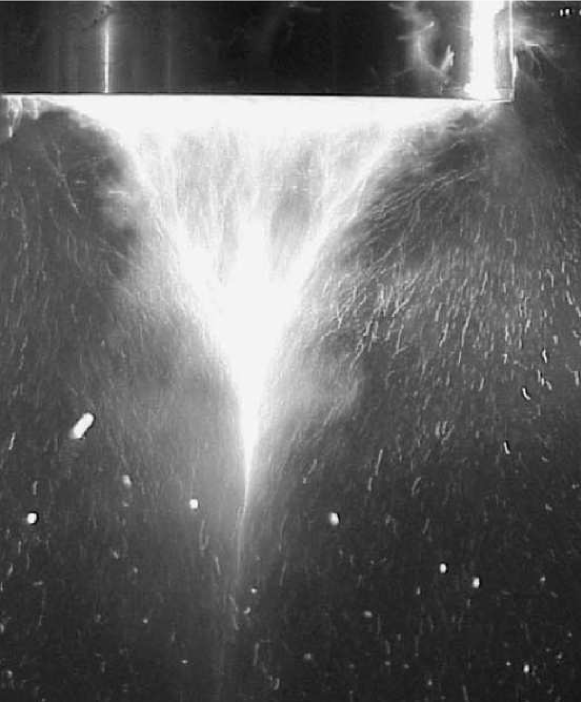
Figure 6: Original image of cone bubble structure (reprinted from Ref. [15], with permission from Elsevier). The transducer diameter is 12 cm.

We present in Fig. 7 a comparison between this picture and the result of our model for $U_{0}=1.4$ $\mu$m and $N_{0}=360$ bubbles.mm^-3. Because the original picture is non-symmetric, and to ensure a maximal objectivity in the comparison, we present our result compared both to the left part of the cone (Fig. 7a) and to its mirrored right part (Fig. 7b). Besides, the original picture has been video-reversed in order to obtain black bubble paths on a white background. We emphasize that this was the only image treatment performed. The Blake threshold contour curve is displayed in thick solid red line. The S-streamers, originating from the transducer, are displayed in black, while the L-streamers, originating from arbitrary points on the Blake threshold contour line are displayed in blue.

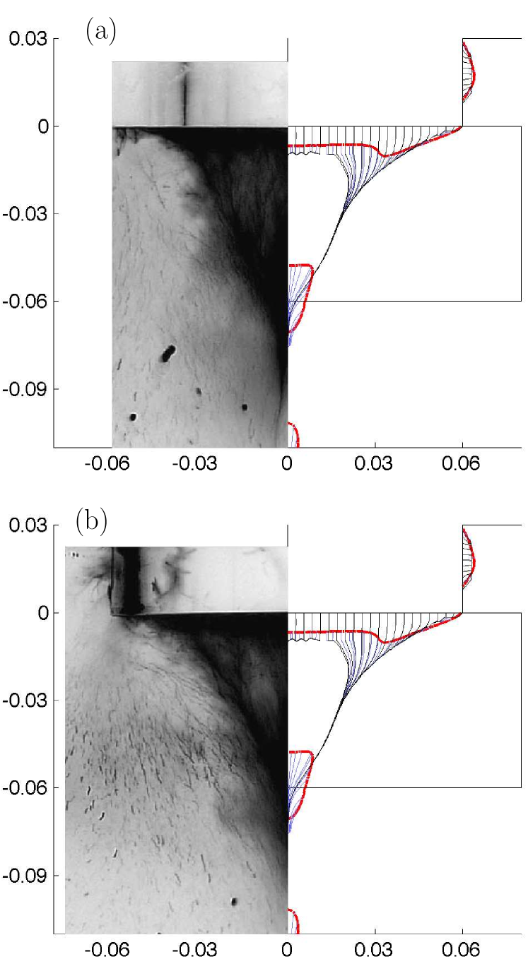
Figure 7: Comparison between the experimental picture of Fig. 6 (the image of Ref [15] has been video reversed in order to make the comparison easier) and the numerical results obtained for 2 $\mu$m air bubbles, with $U_{0}=1.4$ $\mu$m, $N_{0}=360$ bubbles.mm^-3. The input intensity is 8.2 W.cm^-2. The black lines are the S-streamers, the blue lines are the L-streamers, and the thick solid red line is the Blake threshold contour curve ($|P^{*}|=1.178$ for 2 $\mu$m bubbles). (a) comparison with the left part of Fig. 6 ; (b) comparison with the mirrored right part of Fig. 6. The horizontal and vertical lines in the liquid just mark the separation between various subdomains and do not have any physical meaning.

First, it is seen that the global shape of the cone is correctly reproduced. The acoustic pressure on the axial point of the emitter is 2.16 bar. Cavitation occurring near the sonotrode dissipates a lot of energy, which produces a strong attenuation and therefore a large traveling wave contribution in the vertical direction. Bubbles originating from the transducer (black lines in Fig. 7) are therefore strongly expelled from the sonotrode surface, the mechanism being the same as the one explained above for 1D waves (see Fig. 4).

A more detailed analysis of the vertical component of the Bjerknes force can be made by referring to the $z$-projection of Eq. (11). The green line in Fig. 8 represents the standing wave contribution $I_{C}\cos\left[\phi(\mathbf{r})-\psi_{z}(\mathbf{r})\right]$ as a function of the distance to the sonotrode (the latter being located on the right of the graph), the red line is the traveling wave contribution $I_{S}\sin\left[\phi(\mathbf{r})-\psi_{z}(\mathbf{r})\right]$, and the blue line is the sum of the two latter. The sign of the blue line represents therefore the sign of the $z$-component of $\mathbf{F_{B}}$, which, if negative, corresponds to a downward oriented force. It can be seen that near the sonotrode, the vertical Bjerknes force is dominated by the strong repulsive traveling wave contribution, as was the case for the 1D simulation, which is clearly due to the strong attenuation of the wave near the sonotrode. It can be noticed by the way that the standing wave contribution is repulsive only in a small layer near the sonotrode because the acoustic pressure is larger than the threshold 1.7 bar in this zone. Then, slightly before $z=-0.01$ m, the positive standing wave contribution cancels exactly the traveling wave one, and becomes dominant, so that the Bjerknes force becomes positive. This means that, as far as only the $z$-component of the Bjerknes force is concerned, there is a stagnation point for bubbles near $z=-0.01$ m. In fact as will be seen below, this point is a saddle-point since the axis is repulsive in the radial direction at this point, so that the bubbles expelled from the sonotrode brake here in the $z$-direction and follow their motion radially, which explains the formation of the void region in the core of the cone. Near $z=-0.02$ m, the standing wave contribution changes sign again, so that the force becomes downwards and dominated by the traveling wave again. Drawing the same curves for larger distances from the sonotrode would show that this is the case up to another sign-change of the standing wave contribution, near $z=-0.155$ m, which constitutes a real stagnation point since there, the radial force is oriented towards the axis. Contrarily to earlier interpretations [14, 1], the present results suggest that the tip of the cone (near $z=-0.07$ m) is not a stagnation point, and that the real one is located well below, so that the bubbles follow closely the axis up to the latter on an appreciable distance. This is consistent, at least qualitatively, with the original picture of the cone Fig. (6) which shows that the cone ends into a long fluctuating tail.

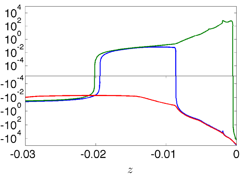
Figure 8: Blue line: magnitude of the parenthesis of $\mathbf{F_{B}}_{z}$ in Eq. (11) along the symmetry axis. The emitter is on the right of the graph. Green line: $\cos$ term in the parenthesis of $\mathbf{F_{B}}_{z}$ in Eq. (11) (standing wave contribution). Red line: $\sin$ term in the parenthesis of $\mathbf{F_{B}}_{z}$ in Eq. (11) (traveling wave contribution).

We now look at the behavior in the radial direction. Figure 9 displays $\sin^{2}\theta_{r}$, where $\theta_{r}=\phi(\mathbf{r})-\psi_{r}(\mathbf{r})$ is the phase shift between $p$ and $\partial p/\partial r$. It can be seen that a large region of traveling wave in the r-direction ($\sin^{2}\theta_{r}\simeq 1$) surrounds approximately the cone boundary, but that $\sin^{2}\theta_{r}$ decreases back to zero when either entering the core of the cone, or moving outward perpendicular to the cone boundary. In the latter two regions, the wave has therefore a larger standing part, so that the classical picture of attraction by pressure antinodes and repulsion by pressure nodes applies. Thus, when the pressure is maximal on the axis, bubbles converge toward the latter, and this explains the formation of the narrow cone tip. This is the case for $z=-0.04$ m (thin solid line in Fig. 10). The opposite holds in the core of the cone, where the variations of the acoustic pressure in the radial direction presents a local minimum on the axis, for example at $z=-0.01$ m (dashed line in Fig. 10) or $z=-0.02$ m (dash-dotted line). The radial component of the Bjerknes force in this zone is therefore oriented outwards. This is why, as mentioned above, the point on the axis (near $z=-0.01$ m) where the $z$-component of the Bjerknes force change sign is in fact a saddle-point, which locally pushes the bubbles far from the axis, and produces a void region in the heart of the cone, clearly visible on the experimental picture. This feature has been commented in Ref. [15] and was attributed to the nonlinear reversal of the Bjerknes force in standing waves near 1.7 bar. Our results suggest that this is not the case, and that the void region results from a combination of a canceling $z$-component of the Bjerknes force and a local inversion of the radial standing wave pressure profile.

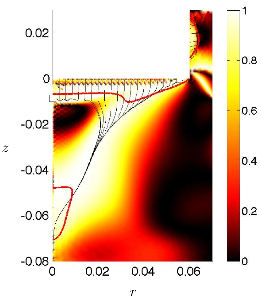
Figure 9: Color plot of $\sin^{2}\theta_{r}$, where $\theta_{r}$ represents the phase between $p$ and $\partial p/\partial r$. The S-streamers are recalled in black lines.

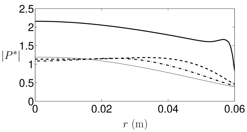
Figure 10: Radial pressure profiles at $z=0$ m (thick solid line), $z=-0.01$ m(dashed line), $z=-0.02$ m (dash-dotted line), $z=-0.04$ m (thin solid line).

The shape of our predicted void region shows reasonable agreement with the experiments. Furthermore, the experimental cone tip seems to be more dense than its core. This may be due to nucleation of bubbles at the Blake threshold in this part, as suggested by the L-streamers starting from the Blake contour loop just above the cone tip in Fig. 7 (blue lines).

Another common observation on such sonotrodes is the presence of small streamers on their lateral side, visible near the upper left corner of Fig. 7b. As seen in the right part of the latter figure, this phenomenon is reasonably caught by the simulation, and this is the reason why the deformation of the transducer was accounted for. Indeed, our result suggests that such small structures result from the lateral vibration of the sonotrode, which emits a radial wave, and produces a small zone of large acoustic pressure. The bubbles in this zone strongly attenuate the wave, and produces a traveling part in the radial wave. The physical mechanism is therefore similar to the cone formation, but here the stagnation point is very close to the sonotrode surface, so that only a small flat filamentary structure is formed.

Figure 11 shows the same result as Fig. 7b where we sketched additional streamers originating from arbitrary points in the liquid (green lines), which makes the comparison of the lateral filamentary structure with experiments more striking. Furthermore, this representation allows to evidence streamers starting near the cone lateral boundary and quickly merging with the latter, as indeed visible on the experimental picture. Figure 11 also shows that the corner of the sonotrode acts as a separatrix between the streamers attracted by the cone and the ones attracted by the lateral filamentary structure, as can be also speculated from the experimental picture. We note however that streamers starting at a larger distance from the cone (see magenta lines in Fig. 11) start upwards, whereas such streamers on the experimental picture seems to start downwards. The experimental image also suggests that some streamers starting from points far from the cone (say, near $r=0.06$ m, $z=-0.07$ m) seem to be attracted by points located outside the picture, and this feature is not caught by our simulation.

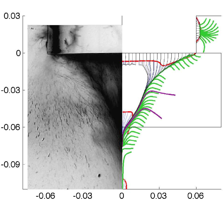
Figure 11: Same as Fig. 7b, sketching additional streamers originating from arbitrary points points below the Blake threshold (green and magenta lines).

The interpretation of the cone structure as the result of the combination of a longitudinal traveling wave and a lateral standing wave proposed in Ref. [14] is therefore confirmed by the present model. However, the above analysis does not tell much about how such an acoustic field appears. Since cone bubble structure are very robust against amplitude, sonotrode size (see discussion in Ref. [15]), and even appear near the walls of ultrasonic baths (see Ref. [1], and next section), there must be some generic mechanism responsible of its formation. Since traveling waves constitute the key phenomenon of the problem, it is interesting to sketch the contour lines of the acoustic field phase ($\phi$ in Eq. (3)). For a traveling wave these lines are orthogonal to the direction of propagation and constitute therefore a powerful visual tool to assess the latter. The result is displayed in Fig. 12 (white lines). It can be seen that, while the wave mainly propagates along the $z$-direction inside the cone, it bends into an oblique direction near the cone boundary, targeting at a point located on the symmetry axis (S-streamers are recalled in black). We emphasize that the emission of an oblique wave from the sonotrode corner was found to occur in all our simulations, whatever the sizes of the sonotrode and the liquid domain, and the type of the bottom liquid boundary. More importantly, we found that the same phenomenon occurs whenever the deformation of the sonotrode was accounted for or not, which rules out any effect of a non uniform displacement of the sonotrode tip.

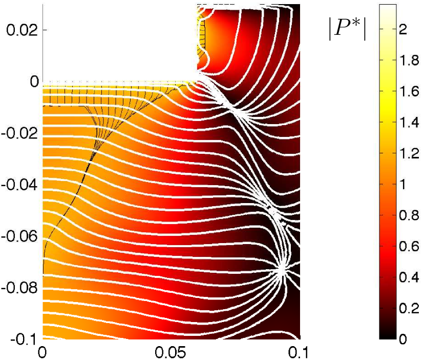
Figure 12: Color plot of the acoustic pressure field in the liquid. The white lines are the contour lines of the phase $\phi$ of the acoustic pressure field (see Eq. (3)). The S-streamers are recalled by the black lines.

We therefore infer that the slanting of the wave propagation direction is definitely linked to the presence of strongly driven bubbles near the vibrating area. These bubbles dissipate a lot of energy, rendering the square of the local wave number almost purely imaginary. But the acoustic field near the outer points of the sonotrode is weaker, because this region is less constrained laterally (see pressure profile in thick solid line in Fig. 10). Therefore, as evidenced in $[$OL I$]$ (see Fig. 4 in the latter reference), the real part of $k$ is higher in the central part of the sonotrode than in its outer part, and the opposite holds for the sound velocity $\omega/\Re(k)$, which is confirmed by Fig. 13. There appears therefore an outward gradient of sound speed along the sonotrode area, which, following Huygens principle, bends the wave number towards the axis, and produces the conical traveling wave visible on Fig. 12. This traveling wave produces in turn a strong Bjerknes force directed along the propagation direction of the wave (a large $I_{S}$ term in Eq. (11)), which structures the bubbles into a conical shape. The latter scenario was qualitatively checked by simple linear acoustics simulations: setting the sound field to $c_{l}$ uniformly in the liquid except in a thin cylinder-shaped region below the transducer, the bending of the iso-$\phi$ lines was indeed observed.

Figure 13: Radial profile of sound velocity on the transducer area. The sound velocity is non-dimensionalized by the sound velocity in the pure liquid $c_{l}$.

A remarkable feature of cone bubble structures is the invariance of their shape when intensity is increased above a given level [15]. Following the suggestion of an anonymous reviewer, we performed an additional simulation of the above configuration, increasing the sonotrode displacement $U_{0}$ up to 4.2 $\mu$m (instead of 1.4 $\mu$m). The results are presented as supplementary material. The cone shape obtained is indiscernible from the one presented in Fig. 11. However, a close examination of the axial pressure profiles in the two cases reveals that the acoustic fields differ mainly in a thin layer of about 5 mm near the sonotrode (see supplementary material). This is a clear manifestation of the self-saturation effect inherent to the present model through the field-dependence of the attenuation coefficient (see $[$OL I$]$): increasing the sonotrode displacement produces a large increase of acoustic pressure only locally, but the bubbles in this zone being excited more strongly, they dissipate the excess acoustic energy very rapidly. It should be noted that experimental manifestations of this phenomenon have been reported in the early work of Rozenberg [35].

Other studies demonstrates that conversely, for low excitations, the shape of the cone bubble structure does depend on the driving. Although some of our simulations could partially catch such a dependence, convergence problems in this range prohibited any firm conclusion. We observed however that the cone shape was very sensitive to the choice of the bubble density when the latter was low enough. This might suggest that the experimentally observed shape dependence for low drivings would be rather due to the variation of the bubble density with acoustic pressure, than to the pressure dependence of a single bubble dissipation. This is a missing brick in our model since we consider constant bubble densities above the Blake threshold. We thus infer that the model in its present form is not able to catch the latter experimental feature.

One should finally mention, as underlined in Ref. [28], another explanation for the cone structure robustness against driving level above a certain threshold, borrowed to phase transitions theory. Skokov and co-workers measured laser intensity transmission through a cavitation zone and obtained time-series presenting fluctuations whose power spectrum were found to be inversely proportional to frequency [36, 37]. This feature, also termed as “flicker noise” has been shown to occur in various physical processes [38], and has been interpreted as a consequence of the interaction between two phase transitions, one subcritical, the other supercritical [39]. The result is that the system self-organizes into a critical state, whatever the precise value of the controlling parameter, contrarily to classical critical states which require a fine tuning of the latter to be reached. This phenomenon has been termed as “self-criticality” and produces organized self-similar spatial structures, reminiscent of bubble web-like organization. Self-criticality can be modeled generically by a stochastic dynamical system of two equations, generalizing the Ginzburg-Landau equation. One of the two order parameters exhibits fluctuations between two attractors, with a power spectrum varying in $1/f$, as observed in experiments. This original theory has the advantage to explain some generally overlooked features of cavitation clouds by a universal physical mechanism. However it still remains very far from the precise cavitation physics, and the proposed equations are phenomenological. In particular the precise physical sense of the order parameters remains to be explicited, maybe on the light of the coupled evolutions of the bubble field and the acoustic wave. For now, the model is still far from a predictive tool for acoustic cavitation, but this promising approach remains opened.

3.3.2 Experiments with a 7 cm diameter sonotrode

Reference [15] also present results for thinner sonotrodes, but the latters produce acoustic currents which deform the cone structure, so that a direct comparison of the experimental images and simulated cone structures is not possible in this case. In spite of the latter restriction, we performed additional simulations for a 8 mm diameter sonotrode (referred as “type B” in Ref. [15]), in an otherwise identical geometry, for 2 $\mu$m bubble radii and a bubble density $N_{0}=$ 90 bubbles/mm³, in order to match at best the experimental shape of the cone structure. The result of the visual comparison between the simulated cone structure and Fig. 2 in [15] is deferred to supplementary material, and shows that, in spite of the blurring of the structure by acoustic currents, some similarities in the cone shape can be observed.

Apart from imaging cone structures, Dubus and co-workers have collected valuable quantitative experimental informations in additional studies, using 7 cm diameter sonotrodes excited in pulsed mode in order to avoid acoustic currents [16, 28]. In order to put our model to the test, we performed additional simulations of a 7 cm sonotrode, again with for 2 $\mu$m bubble radii and $N_{0}=$ 90 bubbles/mm³. The transducer displacement was set in order to match the velocity of the sonotrode area measured in Ref. [16] (1.31 m/s). It is interesting to compare the calculated and experimental axial acoustic pressure profiles (Fig 6 in Ref. [16], star signs). The result is displayed in Fig. 14. It can be seen that the agreement is somewhat poor: even if the order of magnitude of the predicted pressure field is reasonable, it vanishes much more slowly than the experimental one. We increased the bubble density up to $N_{0}=$ 360 bubbles/mm³ without appreciable change in the pressure profile, except near the sonotrode. This underlines the limit of the present model, and may result of the rough assumption of a constant bubble density. Besides, the pressure field calculated in the immediate vicinity of the transducer ($z=0$) is found to be much larger than the experimental one. It should however be noted that hydrophones have a finite size, which does not allow to measure the acoustic pressure exactly near $z=0$, where the present theory predicts a large pressure gradient.

Figure 14: Pressure profile on the symmetry axis for a 7 cm diameter sonotrode, with $R_{0}=2$ $\mu$m, $N_{0}=90$ bubbles/mm³. The velocity of the sonotrode tip is 1.31 m/s. Solid line: prediction by the present model. Stars: experimental measurements redrawn from Fig. 6 in Ref. [16].

Finally, Dubus and co-workers [28] proposed an alternative explanation of the bubble cone structure. Their analysis relies on the formation of a nonlinear resonant layer of bubbly liquid attached on the transducer, the focusing being qualitatively attributed to the curvature of the bubble layer. This layer produces a phase shift of the wave emitted by the sonotrode, dependent on its local width. The argumentation is supported by phase measurements of the pressure field in a horizontal plane below the layer. We have therefore reported the corresponding experimental values, along with the prediction of our simulation in Fig. 15 (the simulation parameters are the same as for Fig. 14). It can be seen that the agreement is very good, and the result was found almost unsensitive to an increase of the bubble density up to $N_{0}=$ 360 bubbles/mm³.

Figure 15: Radial variation of the phase of the pressure field, at 1.5 cm from the transducer. The quantity represented is $(\phi(0,1.5\text{ cm})-\phi(r,1.5\text{ cm}))/(2\pi)$, where $\phi(r,z)=\arg(p(r,z))$. The solid line represents the theoretical prediction, and the stars are experimental results redrawn from Fig. 10 in Ref. [28]. The simulations parameter are the same as for Fig. 14.

The present calculation shows therefore that the existence of a curved resonant layer of bubble is not necessary to explain the experimental results, although nonlinear resonant effects cannot be discarded. The wave focuses anyway just because the outermost bubbles in the bubble layer are more smoothly driven than the central ones, and therefore have a lower influence on the local sound speed. This a purely nonlinear effect, and is correctly summarized by Fig. 4 in $[$OL I$]$. Besides, our simulations indeed exhibit a bubbly layer near the transducer, but rather than being resonant, this layer is in fact found to be very dissipative. Such a large dissipation cannot be predicted by using a reduced bubble dynamic equation, and is strongly correlated to the inertial character of the bubble oscillations, as shown in our companion paper $[$OL I$]$.

3.4 Cleaning bath

The system considered is axi-symmetrical and is represented in a half-plane cut on Fig. 16. The bottom of the bath is a thin circular steel plate of 4 mm thickness and 20 cm diameter, which upper side is in contact with the liquid, while its lower side is free, except its central part (red line on Fig. 16, $r\in[0,3$ cm$]$) which is assumed to vibrate with a uniform amplitude $U_{0}=2$ $\mu$m and a frequency of 20 kHz. This boundary condition is a simplification of a system where a piezo-ceramic ring would be clamped to the bottom side of the plate and impose an oscillatory displacement. The liquid fills the space above the plate, and is limited laterally by a cylindrical boundary, which is assumed infinitely rigid, while the free surface is considered as infinitely soft. The plate is assumed elastic and its deformation follows the Hooke’s law, its vibrations being coupled to the acoustic field in the liquid by adequate interface conditions [30].

Figure 16: Geometry and meshing of the cleaning bath configuration. The geometry has axial symmetry and only a half-plane cut is represented. The blue line is the symmetry axis. A uniform displacement $U_{0}$ is imposed on the red line.

Fig. 17 displays the result obtained with 5 $\mu$m air bubbles and a water height of 0.14 m. The green line represents the deformed shape of the bottom plate, and shows that a flexural standing wave is excited in the latter. This flexural wave produces a spatially inhomogeneous acoustic pressure field on the plate area, ranging in this case between 0.5 and 2.8 bar (the red lines represent the Blake threshold contour curves). In the zones on the plate where the acoustic pressure is larger than the Blake threshold, bubbles are produced, dissipating locally a large energy and modifying the sound speed. The remaining mechanisms are similar to the cone bubble structure described above. Dissipation produces traveling waves, and and can even result into the production of a small cone bubble structure (near $r=0.04$ m) attached on the plate, while other structures on the plate are more similar to the above-mentioned streamers attached on the lateral side of sonotrodes. A few streamers are also visible in the middle of the liquid, located on the antinodes of the wave, which again takes a standing character in this region.

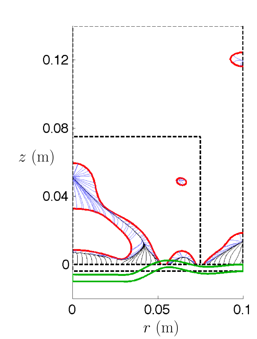
Figure 17: Simulation of the cleaning bath configuration. The thick red lines materialize the Blake-threshold. The black lines are the S-streamers, paths of bubbles originating from the vibrating plate, and the blue lines are the L-streamers, path of bubbles originating from the Blake threshold. The green thick line represents the deformed shape of the plate at $\omega t=2n\pi$.

An interesting feature can also be seen in Fig. 17 and is magnified in Fig. 18b. It is seen that the S-streamers (black lines) merging at the vertex of the cone then follow a unique path up to a stagnation point located on the symmetry axis. If we also launch bubbles from the Bjerknes contour curves, the corresponding L-streamers (blue lines) join the main S-streamers up to the stagnation point where numerous secondary streamers end up, forming a star-like structure. The experimental occurrence of this behavior has been reported in a detailed presentation by Mettin [1], who termed this bubbles arrangement as “flare structure”, and is represented in Fig. 18a). It is seen that, apart from the curvature of the structure observed in our simulation, the latter reproduces reasonably well the main features of the phenomenon, especially the cone structure attached to the vibrating plate merging into a jet, fed laterally by bubbles originating in the bulk liquid. Mettin reported that this structure was universally found in cleaning bath setups and proposed a qualitative explanation involving a “complicated near field structure with shares of both traveling and standing waves”. The present results seem to enforce this interpretation: a traveling wave takes birth near the vibrating area, because of the strong attenuation by the bubbles located there, and launches the bubbles far from the plate. It ends up at a pressure antinode which attracts all the bubbles, either coming from the plate, or taking birth in neighboring zones. The lateral enrichment of the main bubble path originates from a standing wave in the direction perpendicular to the traveling wave.

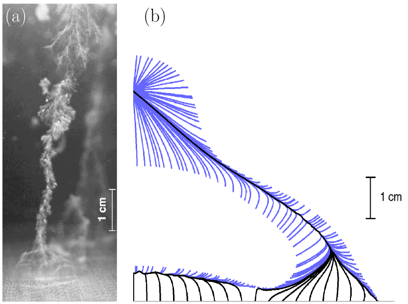
Figure 18: Comparison between: (a) a flare structure observed on the lateral side of a cleaning bath (reprinted from Ref. [1] with permission of Research Signpost; the original image has been 90^∘ rotated for comparison purposes) (b) the structure predicted in the simulated configuration (zoom of Fig. 17 with more L-streamers sketched).

4 Summary and discussion

The model proposed in the companion paper $[$OL I$]$ has been applied to classical 2D configurations, namely large area transducer emitting in a liquid, and cleaning baths. The density of bubbles was assumed constant in zones where the acoustic pressure is above the Blake threshold, and null everywhere else. The possible paths of the bubbles were assumed to originate either from the vibrating parts of the solid, or from the Blake threshold contour curves, and calculated by computing the primary Bjerknes force field directly from nonlinear bubble dynamics simulations.

In the case of large area transducer, cone bubble structures observed experimentally can be easily reproduced, with reasonable agreement in the cone shape. A strongly dissipative bubble layer was found to appear near the transducer, and the cone boundaries were shown to be made of bubbles following a focused traveling wave. The focusing was found to result from a radial acoustic pressure gradient on the transducer area, which, following the result of the companion paper $[$OL I$]$ produces a radial gradient of sound velocity. The streamers located on the lateral boundary of the transducer, observed experimentally, were correctly reproduced by our simulations, provided that the elastic deformations of the emitting transducer were accounted for. Besides, the calculated stagnation point on the symmetry axis was found to be much farther than the cone tip, which would explain the long bubble tail visible in experimental picture.

In the cleaning bath configurations, the flexural vibrations of the bottom plate were found to produce several zones of large acoustic pressures, located near the plate displacement antinodes. These high acoustic pressures produce locally a thin layer of strongly oscillating bubbles dissipating a lot of acoustic energy, which yields damped traveling waves and cone-like structures. In some cases, the bubbles reaching the cone tip carry on their motion along a unique line, ending into a distant pressure antinode, and laterally enriched by bubbles originating from liquid zones excited above the Blake threshold. The obtained structure is reminiscent of a flare-like structure described in the literature, and known to occur frequently in cleaning baths configurations.

The reasonable success of our model in predicting ab initio such structures is encouraging, and seem to show that strong energy dissipation by inertial bubbles is a key mechanism ruling the structure of the acoustic field in a cavitating medium. It is interesting to note that the self-action of the acoustic field evidenced in the present paper differs from the mechanisms presented in the work of Kobelev & Ostrovski [40]. In the latter work, the self-action of the acoustic field is mediated by its slow influence on the bubble population, while here, the mechanism is only due to the bubbles radial motion, even for constant bubble density. The latter assumption constitutes however a weak point of our model, and requires the arbitrary choice of two free parameters: the ambient radius of the bubbles $R_{0}$, and the bubble density, both being assumed spatially homogeneous in regions above the Blake threshold. A more realistic model would require at least the spatial redistribution of the bubbles. This may be done for example by coupling the nonlinear Helmholtz equation used in this paper with a convection-like equation for the bubble number density, as done in the linear case in Ref. [40], which requires the correct estimation of the average translational velocity of inertial bubbles. As already mentioned in introduction, this translational motion is described by a somewhat elaborate physics [26, 27], and the estimation of an average velocity raises the complicated issue of properly averaging the translation equation [19, 20, 21]. Along the same line of investigation, an extension of the present work could consist in launching some bubbles in the acoustic fields presented here, and to calculate their paths within the latter by integrating in time the coupled equations of radial and translational motion described in Refs. [25, 27]. Apart from testing the validity of the current approximation, this would also provide a clear picture of the dynamics of bubble drift in the studied structures. This may reveal some unexpected features, such as bubble precession around some points in the liquid, as evidenced in simple standing waves in Ref. [27]. Such refinements may be the subject of future work, keeping however as a main objective a model simple enough to be used in real engineering applications.

Finally, many other bubble structures can be observed experimentally [1]. Among the latter, the grouping of bubbles into so-called “clusters” classically appear in numerous experimental configuration either in the bulk liquid, or as hemi-spherical structures near solid boundaries, especially in the case of focused ultrasound [41, 42, 43]. In some aspects, they behave as a single large bubble and may collapse as a whole, emitting a complex set of primary and secondary shock-waves (see Ref. [43] for high-speed photographs), and yield strongly erosive effects [44]. A complete theoretical description of such structures is not yet available, the difficulty lying in the strong interaction between the bubbles constituting the cloud. Clearly, this interaction cannot be accounted for by our simple model which includes only primary Bjerknes forces. Moreover, these structures often present a transitory behavior, moving as a whole entity in the liquid, appearing and disappearing near other structures [44, 1], and have even been observed as early precursors of conical structures [45]. As a conclusion, we feel therefore that our model in the present form cannot account for such structures.

5 Acknowledgments

The author acknowledges the support of the French Agence Nationale de la Recherche (ANR), under grant SONONUCLICE (ANR-09-BLAN-0040-02) ”Contrôle par ultrasons de la nucléation de la glace pour l’optimisation des procédés de congélation et de lyophilisation”. Besides the author would like to thank Nicolas Huc of COMSOL France for his help in solving convergence issues.

Appendix A Supplementary data

Supplementary data associated with this article can be found, in the online version, at doi:xx.xxxx/x.xxx.xxxx.xx.xx.

References

- [1] R. Mettin, in: A. A. Doinikov (Ed.), Bubble and Particle Dynamics in Acoustic Fields: Modern Trends and Applications, Research Signpost, Kerala (India), 2005, pp. 1–36.
- [2] U. Parlitz, R. Mettin, S. Luther, I. Akhatov, M. Voss, W. Lauterborn, Phil. Trans. R. Soc. Lond. A 357 (1999) 313–334.
- [3] R. Mettin, in: T. Kurz, U. Parlitz, U. Kaatze (Eds.), Oscillations, Waves and Interactions, Universitätsverlag Göttingen, 2007, pp. 171–198.
- [4] V. F. K. Bjerknes, Fields of Force, Columbia University Press, New York, 1906.
- [5] S. A. Zwick, J. Math. Phys. 37 (1958) 246–268.
- [6] I. Akhatov, R. Mettin, C. D. Ohl, U. Parlitz, W. Lauterborn, Phys. Rev. E 55 (3) (1997) 3747–3750.
- [7] J. Magnaudet, I. Eames, Ann. Rev. Fluid Mech. 32 (2000) 659–708.
- [8] T. G. Leighton, A. J. Walton, M. J. W. Pickworth, Eur. J. Phys. 11 (1990) 47–50.
- [9] L. A. Crum, A. I. Eller, J. Acoust. Soc. Am. 48 (1) (1970) 181–189.
- [10] D. F. Gaitan, L. A. Crum, C. C. Church, R. A. Roy, J. Acoust. Soc. Am. 91 (6) (1992) 3166–3183.
- [11] B. P. Barber, R. A. Hiller, R. Löfstedt, S. J. Putterman, K. R. Weninger, Phys. Rep. 281 (1997) 65–143.
- [12] O. Louisnard, Phys. Rev. E 78 (3) (2008) 036322.
- [13] P. Koch, D. Krefting, T. Tervo, R. Mettin, W. Lauterborn, in: Proc. ICA 2004, Kyoto (Japan), Vol. Fr3.A.2, 2004, pp. V3571–V3572.
- [14] P. Koch, R. Mettin, W. Lauterborn, in: D. Cassereau (Ed.), Proceedings CFA/DAGA’04 Strasbourg, DEGA Oldenburg, 2004, pp. 919–920.
- [15] A. Moussatov, C. Granger, B. Dubus, Ultrasonics Sonochemistry 10 (2003) 191–195.
- [16] C. Campos-Pozuelo, C. Granger, C. Vanhille, A. Moussatov, B. Dubus, Ultrasonics Sonochemistry 12 (2005) 79–84.
- [17] A. I. Eller, L. A. Crum, J. Acoust. Soc. Am. 47 (3) (1970) 762–767.
- [18] T. J. Matula, Philos. Trans. R. Soc. London, Ser. A 357 (1999) 225–249.
- [19] A. J. Reddy, A. J. Szeri, J. Acoust. Soc. Am. 112 (2002) 1346–1352.
- [20] D. Krefting, J. O. Toilliez, A. J. Szeri, R. Mettin, W. Lauterborn, J. Acoust. Soc. Am. 120 (2) (2006) 670–675.
- [21] J. O. Toilliez, A. J. Szeri, J. Acoust. Soc. Am. 122 (5) (2008) 3006–3006.
- [22] S. Khanna, N. N. Amso, S. J. Paynter, W. T. Coakley, Ultrasound in Medicine & Biology 29 (10) (2003) 1463 – 1470.
- [23] T. Watanabe, Y. Kukita, Phys. Fluids A 5 (11) (1993) 2682–2688.
- [24] A. A. Doinikov, Phys. Fluids 14 (4) (2002) 1420–1425.
- [25] A. A. Doinikov, Phys. Fluids 17 (128101) (2005) 1–4.
- [26] A. A. Doinikov, Recent Res. Devel. Acoustics 2 (2005) 13–38.
- [27] R. Mettin, A. A. Doinikov, Applied Acoustics 70 (2009) 1330–1339.
- [28] B. Dubus, C. Vanhille, C. Campos-Pozuelo, C. Granger, Ultrasonics Sonochemistry 17 (2010) 810–818.
- [29] S. Hilgenfeldt, M. P. Brenner, S. Grossman, D. Lohse, J. Fluid Mech. 365 (1998) 171–204.
- [30] O. Louisnard, J. Gonzalez-Garcia, I. Tudela, J. Klima, V. Saez, Y. Vargas-Hernandez, Ultrasonics Sonochemistry 16 (2009) 250–259.
- [31] L. A. Crum, Appl. Sci. Res. 38 (3) (1982) 101–115.
- [32] E. A. Neppiras, Phys. Rep. 61 (1980) 159–251.
- [33] T. J. Leighton, The acoustic bubble, Academic Press, 1994.
- [34] O. Louisnard, F. Gomez, Phys. Rev. E 67 (3) (2003) 036610.
- [35] L. D. Rozenberg, in: L. D. Rozenberg (Ed.), High-intensity ultrasonic fields, Plenum Press, New-York, 1971.
- [36] V. N. Skokov, V. P. Koverda, A. V. Reshetnikov, A. V. Vinogradov, Physica A 364 (2006) 63–69.
- [37] V. N. Skokov, A. V. Reshetnikov, A. V. Vinogradov, V. P. Koverda, Acoust. Phys. 53 (2) (2007) 136–140.
- [38] P. Bak, C. Tang, K. Wiesenfeld, Phys. Rev. A 38 (1) (1988) 364–374.
- [39] V. N. Skokov, A. V. Reshetnikov, V. P. Koverda, A. V. Vinogradov, Physica A 293 (1-2) (2001) 1–12.
- [40] Y. A. Kobelev, L. A. Ostrovskii, J. Acoust. Soc. Am. 85 (2) (1989) 621–629.
- [41] L. Hallez, F. Touyeras, J. Y. Hihn, J. Klima, J. Guey, M. Spajer, Y. Bailly, Ultrasonics 50 (2) (2010) 310–317.
- [42] H. Chen, X. Li, M. Wan, S. Wang, Ultrasonics Sonochemistry 14 (2007) 291–297.
- [43] E. A. Brujan, T. Ikeda, K. Yoshinaka, Y. Matsumoto, Ultrasonics Sonochemistry 18 (1) (2011) 59–64.
- [44] D. Krefting, R. Mettin, W. Lauterborn, Ultrasonics Sonochemistry 11 (2004) 119–123.
- [45] A. Moussatov, R. Mettin, C. Granger, T. Tervo, B. Dubus, W. Lauterborn, in: Proceedings of the World Congress on Ultrasonics, Paris (France), 2003, pp. 955–958.