A framework for coupling flow and deformation of the porous solid

Abstract.

In this paper, we consider the flow of an incompressible fluid in a deformable porous solid. We present a mathematical model using the framework offered by the theory of interacting continua. In its most general form, this framework provides a mechanism for capturing multiphase flow, deformation, chemical reactions and thermal processes, as well as interactions between the various physics in a conveniently implemented fashion. To simplify the presentation of the framework, results are presented for a particular model than can be seen as an extension of Darcy’s equation (which assumes that the porous solid is rigid) that takes into account elastic deformation of the porous solid. The model also considers the effect of deformation on porosity. We show that using this model one can recover identical results as in the framework proposed by Biot and Terzaghi. Some salient features of the framework are as follows: (a) It is a consistent mixture theory model, and adheres to the laws and principles of continuum thermodynamics, (b) the model is capable of simulating various important phenomena like consolidation and surface subsidence, and (c) the model is amenable to several extensions. We also present numerical coupling algorithms to obtain coupled flow-deformation response. Several representative numerical examples are presented to illustrate the capability of the mathematical model and the performance of the computational framework.

1. MOTIVATION AND INTRODUCTION

Higher oil prices and increasing awareness of the environmental impact of carbon pollution have motivated substantial interest in carbon-dioxide capture and storage (CCS). There is a growing consensus in both policy circles and in the energy industry that within the next few years, the US federal government will adopt some form of regulation for $\mathrm{CO}_{2}$ emissions [1]. At the same time, it is widely believed that much of the energy supply over the coming decades will continue to come from fossil fuels. Many analysts believe that the only way to reconcile the anticipated growth in the use of fossil fuels with anticipated limits on $\mathrm{CO}_{2}$ emissions is through the development and deployment of carbon-dioxide capture and sequestration.

Of the proposed techniques for abating anthropogenic carbon-dioxide, storage in deep geologic formations is the only method that has gained widespread acceptance for its feasibility [2, 3]. If geological carbon-dioxide sequestration is implemented on the scale needed to make noticeable reductions in atmospheric $\mathrm{CO}_{2}$, a billion metric tons or more must be sequestered annually – a 250-fold increase over the amount sequestered today. Large sedimentary basins are considered best suited to sequester such large volumes of $\mathrm{CO}_{2}$ as they have tremendous pore volume and connectivity and they are widely distributed [4, 5].

The development of energy systems like geological carbon-dioxide sequestration requires the understanding and predictive simulations of complex processes in earth systems. In particular, securing a large volume of carbon-dioxide will require a solid scientific foundation defining the coupled hydrologic-geochemical-geomechanical processes that govern the long term fate of $\mathrm{CO}_{2}$. This path is becoming more dependent on modeling coupled geomechanical, thermal, fluid and chemical processes and the response of natural and engineered systems. Similarly, these models can be utilized to simulate oil and gas reservoirs, advanced recovery from tar sands and shales, underground storage of hydrogen, natural gas and oil, and evaluating aquifers for new water resources. Significant progress in these areas requires new coupled modeling approaches.

Figure 1. Lake Nyos is a deep crater lake in Cameroon (top figure). In 1986, huge amounts of carbon-dioxide gas were released from the lake possibly due to seismic tremors. A mix of carbon-dioxide and water erupted 120 meters above the lake with a speed of roughly 100 kilometers per hour. This displaced oxygen resulting in asphyxiation of more than 1,700 people and 3,000 cattle as far as 23 kilometers from the lake (bottom figure). [Source: http://www.waterencyclopedia.com/]

Unfortunately, there are still a number of unanswered scientific questions regarding deep geological sequestration that critically affect the efficacy and safety of this method. Although a number of studies have been conducted on geochemical interactions within the storage reservoir, and on the flow characteristics of the carbon-dioxide plume, relatively little effort has been devoted towards the reservoir’s structural integrity. The seal created by the cap rock is one of the primary mechanisms that prevents injected carbon-dioxide from escaping back into the atmosphere. Failure of this seal can release large quantities of carbon-dioxide, which will have dire consequences. For example, in 1986 more than 1700 people were killed by the sudden release of geologic carbon-dioxide from lake Nyos in Cameroon (see Figure 1). Although, in the case of lake Nyos, the carbon-dioxide was sequestered naturally, one can learn valuable lessons from this disaster. What happened in lake Nyos is similar to opening a shaken bottle of carbonated soda. As long as the cap is on, the carbon-dioxide gas stays dissolved under pressure. But when the cap is removed, the bubbles (and the soda) rapidly flow out of the bottle. The lake Nyos incident clearly highlights the importance of the structural integrity of the cap rock, and an immediate need for a systematic study along the lines presented in this paper.

It is important to note that very few parallel processing commercial and/or research software tools exist for simulating complex processes such as coupled multiphase flow with chemical transport and geomechanics. Current computational limitations place significant restrictions on realistic problems that can be solved. Predictive computational simulation of the coupled-physics associated with geosystems is a critical enabling technology for their optimal management. A major stumbling block to high-fidelity modeling and simulation of geosystems is the lack of viable, robust, and efficient computational technologies for describing multiphase, multicomponent chemically reactive fluid mixtures in heterogeneous deformable geologic media. The present paper aims at advancing mathematical and numerical modeling, and predictive simulation of flow in deformable porous media under high pressures.

1.1. Main contributions of this paper

Some of the main contributions of this paper are as follows:

1. We have presented a mathematical model based on the theory of interacting continua which is capable of capturing surface subsidence and consolidation of soils. The model is fully coupled, and the interaction between the fluid and the porous solid is modeled through drag-like term and deformation-dependent porosity.

2. We have presented various numerical coupling algorithms, which can be used to obtain the coupled response.

3. We have presented various representative numerical examples illustrating the predictive capabilities of the proposed mathematical model, and the numerical performance of the coupling algorithms.

1.2. Organization of the paper

The remainder of this paper is organized as follows. In Section 2 we give a brief review of the theory of interacting continua. In Section 3 we present a model for the flow of an incompressible fluid in deformable porous solid. In Section 4 we shall present coupling algorithms that will be employed to obtained the coupled flow-deformation response. Several representative numerical results will be presented in Section 5, and conclusions are drawn in Section 6.

2. ELEMENTS OF THE THEORY OF INTERACTING CONTINUA

We shall employ the mathematical framework offered by the theory of interacting continua (TIC), which is sometimes referred to as the theory of mixtures. The basic assumption of the theory of interacting continua is that the constituents can be homogenized and assumed to co-occupy the domain occupied by the mixture. The theory of interacting continua traces its origins to the works of Darcy [6] (also see its English translation by Patricia Bobeck [7]) and Fick [8]. Truesdell later gave the theory a firm mathematical footing (see [9, 10, 11] and several appendices in Reference [12]). We now provide a brief review of the basic equations of the theory of interacting continua. A more detailed treatment can be found in Atkin and Craine [13], Bowen [14], and Bedford and Drumheller [15]. One can also consult texts by Bowen [16], Coussy [17, 18], de Boer [19], Rajagopal and Tao [20], and Voyiadjis and Song [21].

\psfrag{O}{$\delta V$}\psfrag{O1}{$\delta V^{(1)}$}\psfrag{O2}{$\delta V^{(2)}$}\psfrag{ON}{$\delta V^{(N)}$}\includegraphics[scale={0.55}]{Figures/RVE_mod.eps}

Figure 2. Elementary volume of the porous material $\delta V$, and the volume occupied by the $i$-th constituent $\delta V^{(i)}\;(i=1,\cdots,N)$.

In the remainder of the paper, it should be noted that the usual summation convention on repeated indices will not be adopted. Consider a mixture of $N$ components. One of the components can be the porous solid, which will be the case when dealing with a deformable porous solid. A typical particle belonging to each constituent in the reference state is denoted $\boldsymbol{X}^{(i)}\;(i=1,\cdots,N)$. At time $t$, these particles occupy the position $\boldsymbol{x}$. The motion and velocity of each constituent $(i=1,\cdots,N)$ are defined through

$$\boldsymbol{x} =\chi^{(i)}(\boldsymbol{X}^{(i)},t)$$ (1)

$$\boldsymbol{v}^{(i)} =\frac{\partial\chi^{(i)}(\boldsymbol{X}^{(i)},t)}{\partial t}$$ (2)

We denote the gradient and divergence operators with respect to $\boldsymbol{x}$ through $\mathrm{grad}[\cdot]$ and $\mathrm{div}[\cdot]$, respectively. We now define the volume fractions and porosity by considering a representative volume element (RVE) with volume $\delta V$. The volume occupied by the $i$-th component in the RVE is denoted $\delta V^{(i)}$. The volume fraction of the $i$-th component is then defined as follows:

$$\eta^{(i)}:=\frac{\delta V^{(i)}}{\delta V}$$ (3)

By definition, the volume fractions satisfy the following relationship:

$$\sum_{i=1}^{N}\eta^{(i)}(\boldsymbol{x})=1$$ (4)

The porosity of the porous medium is defined as follows:

$$\phi(\boldsymbol{x}):=1-\eta^{(s)}(\boldsymbol{x})$$ (5)

where $\eta^{(s)}(\boldsymbol{x})$ is the volume fraction of the porous solid. Let the mass of the $i$-th component in this RVE be $\delta m^{(i)}$. The true and bulk mass densities of the $i$-th component are, respectively, denoted by $\gamma^{(i)}$ and $\rho^{(i)}$. That is,

$$\gamma^{(i)} :=\frac{\delta m^{(i)}}{\delta V^{(i)}}$$ (6)

$$\rho^{(i)} :=\frac{\delta m^{(i)}}{\delta V}$$ (7)

The bulk mass density of the mixture is defined as follows:

$$\rho(\boldsymbol{x},t) :=\sum_{i=1}^{N}\rho^{(i)}(\boldsymbol{x},t)$$ (8)

The mixture velocity is defined as follows:

$$\boldsymbol{v}(\boldsymbol{x},t) :=\frac{1}{\rho(\boldsymbol{x},t)}\sum_{i=1}^{N}\rho^{(i)}(\boldsymbol{x},t)\boldsymbol{v}^{(i)}(\boldsymbol{x},t)$$ (9)

The diffusion velocity $\tilde{\boldsymbol{v}}^{(i)}(\boldsymbol{x},t)$ of the $i$-th constituent is defined as follows:

$$\tilde{\boldsymbol{v}}^{(i)}(\boldsymbol{x},t)=\boldsymbol{v}^{(i)}(\boldsymbol{x},t)-\boldsymbol{v}(\boldsymbol{x},t)$$ (10)

Let $\alpha(\boldsymbol{x},t)$ be any quantity (scalar, vector, tensor) defined at the point $\boldsymbol{x}$ in the mixture at time $t$. We then define

$$\frac{\mathrm{D}^{(i)}\alpha}{\mathrm{D}t} :=\frac{\partial}{\partial t}\alpha(\boldsymbol{x},t)+\mathrm{grad}\left[\alpha(\boldsymbol{x},t)\right]\cdot\boldsymbol{v}^{(i)}(\boldsymbol{x},t)$$ (11a)

$$\frac{\mathrm{D}\alpha}{\mathrm{D}t} :=\frac{\partial}{\partial t}\alpha(\boldsymbol{x},t)+\mathrm{grad}\left[\alpha(\boldsymbol{x},t)\right]\cdot\boldsymbol{v}(\boldsymbol{x},t)$$ (11b)

The velocity gradient for the $i$-th constituent $\boldsymbol{L}^{(i)}$ and its symmetric part $\boldsymbol{D}^{(i)}$ are, respectively, defined through

$$\boldsymbol{L}^{(i)} :=\mathrm{grad}[\boldsymbol{v}^{(i)}]$$ (12)

$$\boldsymbol{D}^{(i)} :=\frac{1}{2}\left(\boldsymbol{L}^{(i)}+{\boldsymbol{L}^{(i)}}^{T}\right)$$ (13)

We assume the existence of a partial traction vector $\boldsymbol{t}^{(i)}$ and a partial stress tensor $\boldsymbol{T}^{(i)}$ associated with each constituent of the mixture such that

$$\boldsymbol{t}^{(i)}=(\boldsymbol{T}^{(i)})^{T}\boldsymbol{n}_{S}$$ (14)

where $\boldsymbol{n}_{S}$ is the normal to the surface $S$. We define the total traction and total stress through

$$\boldsymbol{t} =\sum_{i=1}^{N}\boldsymbol{t}^{(i)}$$ (15)

$$\boldsymbol{T} =\sum_{i=1}^{N}\boldsymbol{T}^{(i)}$$ (16)

so that we have

$$\boldsymbol{t}=\boldsymbol{T}^{T}\boldsymbol{n}_{S}$$ (17)

2.1. Balance laws for constituents and the mixture

The balance of mass for the $i$-th constituent takes the following form:

$$\frac{\partial\rho^{(i)}}{\partial t}+\mathrm{div}[\rho^{(i)}\boldsymbol{v}^{(i)}]=m^{(i)}$$ (18)

where $m^{(i)}$ is the mass supply for the $i$-th constituent. It is noteworthy that the theory of interacting continua can take into account the possible inter-conversion of mass due to chemical reactions between the constituents. The balance of mass for the mixture as a whole warrants that

$$\sum_{i=1}^{N}m^{(i)}=0$$ (19)

The balance of linear momentum of individual constituents can be written as follows:

$$\rho^{(i)}\frac{\mathrm{D}^{(i)}\boldsymbol{v}^{(i)}}{\mathrm{D}t}=\mathrm{div}[\boldsymbol{T}^{(i)}]^{T}+\rho^{(i)}\boldsymbol{b}^{(i)}+\boldsymbol{i}^{(i)}$$ (20)

where $\boldsymbol{b}^{(i)}$ is the external body force that acts on the $i$-th constituent, and $\boldsymbol{i}^{(i)}$ represents the interactive forces acting on the $i$-th constituent. That is, $\boldsymbol{i}^{(i)}$ arises due to the forces exerted by the other constituents on the $i$-th constituent by virtue of their being forced to co-occupy the domain of the mixture. Constitutive relations need to be specified for these interaction forces and they in general depend on not just the $i$-th constituent but also on the other constituents. Also, it follows from Newton’s third law that

$$\sum_{i=1}^{N}\left(\boldsymbol{i}^{(i)}+m^{(i)}\boldsymbol{v}^{(i)}\right)=\boldsymbol{0}$$ (21)

In the case of a mixture, even in the absence of angular momentum supply, the individual partial stresses need not be symmetric. However, the total stress will be symmetric in the absence of angular momentum supply, i.e.,

$$\sum_{i=1}^{N}\boldsymbol{T}^{(i)}=\left(\sum_{i=1}^{N}\boldsymbol{T}^{(i)}\right)^{T}$$ (22)

We shall assume that the individual partial stresses are symmetric, and hence equation (22) will be satisfied automatically. That is,

$$\boldsymbol{T}^{(i)}=\left(\boldsymbol{T}^{(i)}\right)^{T}\quad\forall i=1,\cdots,N$$ (23)

One can similarly write governing equations for the balance of energy and the second law of thermodynamics. Herein, we shall restrict the studies to isothermal processes, and hence these equations are either trivially satisfied or not coupled with the mechanical aspects of the problem.

3. A MODEL FOR FLUID FLOW IN DEFORMABLE POROUS SOLID

The above framework offered by the theory of interacting continua is quite general and can model a wide variety of interesting phenomena. Herein, however, we shall consider a simplified but representative model for fluid and solid, which will be a special case of the above comprehensive framework. This simplified model will be used in our study on the stability of coupling algorithms. It should be noted that even this simplified model can capture many interesting features in the flow of fluids in deformable solids as discussed later in this paper.

We do not consider chemical reactions, and hence can set

$$m^{(i)}=0\quad\forall i=1,\cdots,N$$ (24)

The constitutive equation for the fluid is taken to be that of a perfect fluid. That is,

$$\boldsymbol{T}^{(f)}=-p^{(f)}\boldsymbol{I}$$ (25)

where $\boldsymbol{T}^{(f)}$ is the stress in the fluid, $\boldsymbol{I}$ is the second-order identity tensor, and $p^{(f)}$ is the pressure in the fluid. We take into account interactions at the fluid-solid interface by including the following drag-like terms:

$$\boldsymbol{i}^{(f)} =\alpha^{(fs)}\left(\boldsymbol{v}^{(f)}-\boldsymbol{v}^{(s)}\right)$$ (26a)

$$\boldsymbol{i}^{(s)} =\alpha^{(sf)}\left(\boldsymbol{v}^{(s)}-\boldsymbol{v}^{(f)}\right)$$ (26b)

By Newton’s third law (21), we have $\alpha^{(fs)}=\alpha^{(sf)}$. The drag term models the friction between the fluid and the porous solid, and it does not consider the friction within the fluid. The drag coefficient $\alpha^{(fs)}$ can be written as follows:

$$\alpha^{(fs)}=\frac{\mu^{(f)}}{k}$$ (27)

where $\mu^{(f)}$ is the coefficient of viscosity of the fluid, and $k$ is permeability. In this paper, we shall allow the coefficient of viscosity is allowed to depend on the pressure, and is modeled using Barus formula [22, 23]:

$$\mu^{(f)}\left(p^{(f)}\right)=\mu^{(f)}_{0}\exp\left[\beta^{(f)}p^{(f)}\right]$$ (28)

where $\beta^{(f)}$ has units of $\mathrm{Pa}^{-1}$. The values of $\mu^{(f)}_{0}$ and $\beta^{(f)}$ of various organic liquids can found in references [24, 22]. It is straightforward to show that the balance of linear momentum, given in equation (20), becomes

$$\rho^{(f)}\left(\frac{\partial\boldsymbol{v}^{(f)}}{\partial t}+\mathrm{grad}[\boldsymbol{v}^{(f)}]\boldsymbol{v}^{(f)}\right)+\alpha^{(fs)}\left(\boldsymbol{v}^{(f)}-\boldsymbol{v}^{(s)}\right)+\mathrm{grad}[p^{(f)}]=\rho^{(f)}\boldsymbol{b}^{(f)}$$ (29)

Remark 3.1.

A simple model that takes into account the friction between the layers of the fluid has been proposed by Brinkman [25]. The model is referred to as Brinkman equation or sometimes Darcy-Stokes equation. Under this model, the partial stress in the fluid takes the following form:

$$\boldsymbol{T}^{(f)}=-p^{(f)}\boldsymbol{I}+2\mu^{(f)}\boldsymbol{D}^{(f)}$$ (30)

In such a case, the above expression for balance of linear momentum (29) should be altered as follows:

$$\rho^{(f)}\left(\frac{\partial\boldsymbol{v}^{(f)}}{\partial t}+\mathrm{grad}[\boldsymbol{v}^{(f)}]\boldsymbol{v}^{(f)}\right)+\alpha^{(fs)}\left(\boldsymbol{v}^{(f)}-\boldsymbol{v}^{(s)}\right)+\mathrm{grad}[p^{(f)}]-\mathrm{div}[2\mu^{(f)}\boldsymbol{D}^{(f)}]=\rho^{(f)}\boldsymbol{b}^{(f)}$$ (31)

The fluid is assumed to be incompressible, and hence the balance of mass for the fluid can be written as follows:

$$\frac{\partial\phi}{\partial t}+\mathrm{div}\left[\phi\boldsymbol{v}^{(f)}\right]=0$$ (32)

where $\phi$ is the porosity of the porous media. It should be noted that the formulation can be easily extended to variable density flows. We shall model the subsurface rock as a linearized elastic material. That is,

$$\mathop{\mathrm{max}}_{\boldsymbol{x},t}\;\big{\|}\mathrm{grad}[\boldsymbol{u}^{(s)}]\big{\|}_{*}\ll 1$$ (33)

where $\|\cdot\|_{*}$ denotes the trace norm [26], which is defined as follows:

$$\|\boldsymbol{A}\|_{*}=\mathrm{tr}\left[\sqrt{\boldsymbol{A}^{T}\boldsymbol{A}}\right]$$ (34)

where $\boldsymbol{A}$ is a second-order tensor, and $\mathrm{tr}[\cdot]$ denotes the trace. The (linearized) strain in the porous solid is given by

$$\boldsymbol{\epsilon}^{(s)}:=\frac{1}{2}\left(\mathrm{grad}[\boldsymbol{u}^{(s)}]+\mathrm{grad}[\boldsymbol{u}^{(s)}]^{T}\right)$$ (35)

Note that the velocity of the solid is given by

$$\boldsymbol{v}^{(s)}=\frac{\partial\boldsymbol{u}^{(s)}}{\partial t}$$ (36)

The governing equation for the balance of linear momentum for the porous solid takes the following form:

$$\rho^{(s)}\frac{\partial^{2}\boldsymbol{u}^{(s)}}{\partial t^{2}} -\alpha^{(fs)}\left(\boldsymbol{v}^{(f)}-\boldsymbol{v}^{(s)}\right)-\mathrm{div}[\boldsymbol{T}^{(s)}]=\rho^{(s)}\boldsymbol{b}^{(s)}$$ (37)

where $\boldsymbol{u}^{(s)}$ is the displacement of the solid. Note that the interaction effect has opposite signs in the two balance equations (29) and (37) in virtue of Newton’s third law. The constitutive equation for the porous solid can be written as follows:

$$\boldsymbol{T}^{(s)}=\lambda^{(s)}\mathrm{tr}[\boldsymbol{\epsilon}^{(s)}]\boldsymbol{I}+2\mu^{(s)}\boldsymbol{\epsilon}^{(s)}$$ (38)

where $\boldsymbol{T}^{(s)}$ is the stress in the porous solid, and $\lambda^{(s)}$ and $\mu^{(s)}$ are the Lamé parameters of the porous solid. A few remarks about the above mathematical model are in order.

Remark 3.2.

The partial stresses for the fluid (given by equation (25)) and for the solid (given by equation (38)) are symmetric, which is in accordance with the assumption discussed in the previous section.

Remark 3.3.

Equations (29), (32) and (37) are coupled and are in terms of three unknowns: $p^{(f)}$, $\boldsymbol{v}^{(f)}$, and $\boldsymbol{u}^{(s)}$. In some of the specialized models discussed below, the number of unknowns can be reduced by substituting one or more of the equations in the above system into the other equations.

3.1. Quasi-static models

One popular approach to incorporate the influence of the fluid motion on the deformation of the solid and vice versa is by modeling the porosity of the porous media to be dependent on the deformation gradient in the solid. Typically, in this scenario, a number of approximations are made which are necessary to model the balance of momentum for the fluid using Darcy’s law. If we ignore inertia in both the fluid and the solid, we can drop the first term in equations (29) and (37). Similarly, if we assume that the solid velocity is much smaller than the fluid velocity, the interaction term (second term in equations (29) and (37)) may be written as $\alpha^{(f)}\boldsymbol{v}^{(f)}$.

Darcy’s equation can be substituted into the interaction term for the fluid velocity. Rather than replace the interaction, $-\alpha^{(fs)}\boldsymbol{v}^{(f)}$, with the gradient of the fluid pressure, $\mathrm{grad}[p^{(f)}]$, and the fluid body force, $-\rho^{(f)}\boldsymbol{b}^{(f)}$, we shall incorporate the influence of the fluid pressure in the solid stress tensor as

$$\boldsymbol{T}^{(s)}=\boldsymbol{T}_{e}^{(s)}+\boldsymbol{T}_{p}^{(s)}$$ (39)

where $\boldsymbol{T}_{p}^{(s)}=-p^{(f)}\boldsymbol{I}$. Partially incorporating the interaction term due to the fluid pressure in the solid stress as above is possible due to the following relationship, $\mathrm{grad}[p^{(f)}]=-\mathrm{div}[\boldsymbol{T}_{p}^{(s)}]$. The fluid body force, $\rho^{(f)}\boldsymbol{b}^{(f)}$, must of course be taken into account.

3.2. Steady-state response

The governing equations for steady-state response of flow of an incompressible fluid in a deformable porous solid can be written as follows:

Governing equations for fluid

$$\alpha^{(fs)}(p^{(f)})\boldsymbol{v}^{(f)}+\mathrm{grad}[p^{(f)}]=\rho^{(f)}\boldsymbol{b}^{(f)}$$ (40a)

$$\mathrm{div}[\phi\boldsymbol{v}^{(f)}]=0$$ (40b)

Governing equations for solid

$$\mathrm{div}[\boldsymbol{T}^{(s)}]+\alpha^{(fs)}(p^{(f)})\boldsymbol{v}^{(f)}+\rho^{(s)}\boldsymbol{b}^{(s)}=\boldsymbol{0}$$ (40c)

$$\boldsymbol{T}^{(s)}=\lambda^{(s)}\mathrm{tr}[\boldsymbol{\epsilon}^{(s)}]\boldsymbol{I}+2\mu^{(s)}\boldsymbol{\epsilon}^{(s)}$$ (40d)

$$\boldsymbol{\epsilon}^{(s)}:=\frac{1}{2}\left(\mathrm{grad}[\boldsymbol{u}^{(s)}]+\mathrm{grad}[\boldsymbol{u}^{(s)}]^{T}\right)$$ (40e)

Deformation-dependent porosity

$$\phi=\frac{\phi_{0}}{1+(1-\phi_{0})\mathrm{tr}[\boldsymbol{\epsilon}^{(s)}]}$$ (40f)

where $\phi_{0}$ is the porosity when the porous solid is unstrained (i.e., $\mathrm{tr}[\boldsymbol{\epsilon}^{(s)}]=0$). The unknown field variables are: velocity of the fluid $\boldsymbol{v}^{(f)}(\boldsymbol{x})$, pressure in the fluid $p^{(f)}(\boldsymbol{x})$, displacement of the porous solid $\boldsymbol{u}^{(s)}(\boldsymbol{x})$, and porosity $\phi(\boldsymbol{x})$. The above model (given by equations (40a)–(40f)) is nonlinear and fully coupled in the sense that neither the fluid model nor the solid model can be solved independently.

Remark 3.4.

In the literature, one can find many other models for deformation-dependent porosity. For example, the following expression has been proposed:

$$\phi=1-\frac{1-\phi_{0}}{\exp[\mathrm{tr}[\boldsymbol{\epsilon}^{(s)}]]}$$ (41)

Another model, which is used for large deformations of the porous solid, takes the following form:

$$\phi=C_{\phi}\left(1-\frac{(1-\phi_{0})}{\mathrm{det}[\boldsymbol{F}^{(s)}]}\right)$$ (42)

where $\phi_{0}$ is the initial porosity, $\boldsymbol{F}^{(s)}$ is the solid deformation gradient

$$\boldsymbol{F}^{(s)}=\boldsymbol{I}+\mathrm{grad}[\boldsymbol{u}^{(s)}]$$ (43)

and $C_{\phi}$ is a coefficient that may very in time, and can be used to smooth jumps in the porosity in time. In the case where the mass balance equation (equation (40b)) is subcycled, large changes in porosity can occur during synchronization updates. Using a reference pressure, $p_{\mathrm{ref}}$, that is taken as the pressure at the last synchronization update, the following expression can be used to interpolate the porosity between updates

$$C_{\phi}=1+C_{r}(p-p_{\mathrm{ref}})$$ (44)

where $C_{r}$ is the rock compressibility constant.

4. NUMERICAL COUPLING ALGORITHMS

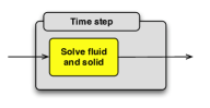
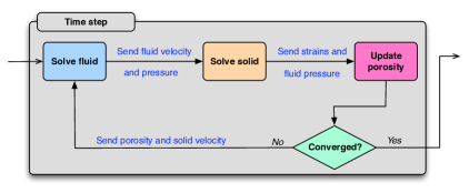
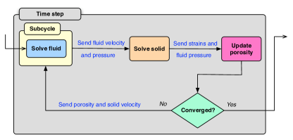
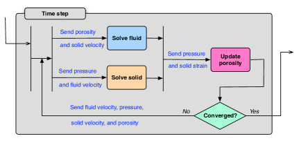
Figure 3. Numerical coupling algorithms: fully coupled (top left), lockstep (top right), subcycling (bottom left), and Jacobi (bottom right).

The coupled equations presented above can be solved in a number of ways, which will depend on how the overall problem is decomposed. The first method is the fully coupled method, which solves governing equations for fluid, solid and porosity update simultaneously as one monolithic system. The variables in this case are solid displacement, fluid velocity, fluid pressure, and porosity. Under this method, it is typical to use the same time step for all subsystems. The second method is the lockstep method (which is also referred to as Gauss-Seidel), which solves each subsystem individually until convergence in serial fashion. The solution is then transferred to the other subsystems which then iterate until convergence. Under the lockstep method, the same time step is also used for all subsystems. In the third method, referred to as the subcycle method, subcycling occurs in either the mass balance or solid deformation equation. For the problems presented below, subcycling was only used for the mass balance equation since the physics of the flow evolves much faster than the solid deformation. The last method considered in this paper is the Jacobi method. Under this method, both equations are decoupled and converged individually, but fields are transferred after each iteration. Figure 3 pictorially describes these coupling algorithms.

5. REPRESENTATIVE NUMERICAL RESULTS

In this section, using the mathematical model described in Section 3, we shall study the performance and relative efficiency of the coupling algorithms that are outlined in the previous section. Several canonical problems are solved.

5.1. Verification by a manufactured solution

In this subsection, we shall use the method of manufactured solutions to verify the implementation of the coupling algorithms. The method of manufactured solutions assumes an exact solution and then derives the corresponding source terms that satisfy the governing equations. The (manufactured) exact solution for the coupled problem (40a)–(40f) takes the following form:

$$u^{(s)}(x)=u_{0}^{(s)}\sin(\pi x),\;\epsilon^{(s)}(x)=u_{0}^{(s)}\pi\cos(\pi x),\;T^{(s)}(x)=\left(\lambda^{(s)}+2\mu^{(s)}\right)u_{0}^{(s)}\pi\cos(\pi x)$$ (45a)

$$v^{(f)}(x)=v_{0}^{(f)}\left(1+(1-\phi_{0})u_{0}^{(s)}\pi\cos(\pi x)\right),\;p^{(f)}(x)=-\alpha^{(fs)}v_{0}^{(f)}\left(x+(1-\phi_{0})u_{0}^{(s)}\sin(\pi x)\right)+p_{0}^{(f)}$$ (45b)

$$\phi(x)=\frac{\phi_{0}}{1+(1-\phi_{0})\mathrm{tr}[\epsilon^{(s)}]}=\frac{\phi_{0}}{1+(1-\phi_{0})u_{0}^{(s)}\pi\cos(\pi x)}$$ (45c)

The prescribed body forces for the fluid and the porous solid are as follows:

$$b^{(f)}(x)=0,\quad b^{(s)}(x)=\frac{u_{0}^{(s)}\pi^{2}}{\rho^{(s)}}\left(\lambda^{(s)}+2\mu^{(s)}\right)\sin(\pi x)$$ (46)

The constants used in this numerical experiment are listed in Table 1.

Table 1. Verification by a manufactured solution: Values used in the numerical simulation.

Parameter	Value	Parameter	Value
$\rho^{(f)}$	1.0	$\rho^{(s)}$	1.0
$v_{0}^{(f)}$	1.0	$p_{0}^{(f)}$	1.0
$\lambda^{(s)}$	1.0	$\mu^{(s)}$	0.5
$\alpha^{(fs)}$	1.0	$\phi_{0}$	0.1
$u_{0}^{(s)}$	0.01

To restrict the analysis of this problem to one-dimension, the boundary conditions are prescribed such that displacements in the $y$-direction are fixed and only displacements in the $x$-direction are considered. The problem domain consists of a unit square with a single element in the $y$-direction and 200 elements in the $x$-direction. On the left side of the domain the solid displacement is fixed. On the right side of the domain, the manufactured solution is applied for the solid displacements as a boundary condition.

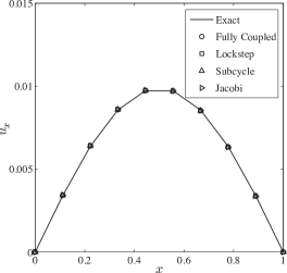
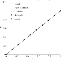
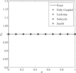
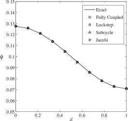
Figure 4. Verification by a manufactured solution: numerical solution vs. $x$ compared with the exact solution (top left) solid displacement, $u_{x}$ (top right) pressure, $p$ (bottom left) fluid velocity, $v_{x}$ (bottom right) porosity, $\phi$. The lockstep method was computed using a tolerance of $\epsilon_{l}=1\times 10^{-9}$. The subcycle method was computed using one subcycle (equivalent to lockstep) and a tolerance of $\epsilon_{s}=1\times 10^{-9}$. The Jacobi method was computed using a tolerance of $\epsilon_{j}=1\times 10^{-9}$.

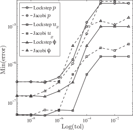
Figure 5. Verification by a manufactured solution: minimum error vs. global convergence tolerance, $\epsilon_{l}$ or $\epsilon_{j}$. The error is measured as the $L_{2}$-norm of the computed solution minus the exact solution and the minimum is taken over the total solution time.

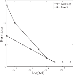
Figure 6. Verification by a manufactured solution: number of iterations vs. global convergence tolerance, $\epsilon_{l}$ or $\epsilon_{j}$. The number of iterations is measured as the number of fluid and solid solves per solution cycle before the global tolerance is met.

The above outlined problem was solved by each of the coupling algorithms described in Figure 3. A comparison between the exact solution and the obtained numerical solution for the fluid pressure, solid displacements, and the porosity are shown in Figure 4. Figures 5 and 6 provide a measure of the efficiency of the loosely coupled algorithms (lockstep and Jacobi). The relative error of the solution is computed as the $L_{2}$ norm of the exact solution minus the computed solution. Notice that both the lockstep and Jacobi methods perform similarly in terms of the accuracy obtained for a given convergence tolerance, but the Jacobi method requires more iterations for a given level of accuracy.

5.2. Terzaghi consolidation problem

To evaluate the performance of the quasi-static model (equations (40a) to (40f)) for one-dimensional transient wave propagation in fluid saturated incompressible porous media we investigate the response of an infinite half-space to time dependent loading. This example problem, which has been studied by a number of researchers including [27, 28], is represented computationally by the domain and parameters shown in Figure 7, although the dimensions of the domain are insignificant regarding the resulting response. The top surface of the domain is subjected to a forcing function, $F$, given as:

$$F=100\left((1-\mathrm{cos}(75t)\right)$$ (47)

The distributed force is applied in a weak fashion over the top surface. This surface is also treated as perfectly drained meaning that the fluid is free to drain from the top surface and the pressure is equal to the ambient pressure. Along the sides and bottom of the domain the fluid is not allowed to drain. The displacement boundary conditions consist of fixing the $x$-displacement along the right and left boundary and the $y$-displacement on the bottom surface. This essentially allows for only one-dimensional consolidation in the $y$-direction.

The analytic solution for the $y$-displacement of the top surface of the domain is given as:

$$u^{(s)}_{y}(t)=\frac{-1.0}{\sqrt{a}(\lambda^{(s)}+2\mu^{(s)})}\int_{0}^{t}F(t-\tau)e^{-\frac{b\tau}{2a}}I_{0}\left(\frac{b\sqrt{\tau^{2}-az^{2}}}{2a}\right)U(\tau-\sqrt{a}z)\;\mathrm{d}\tau$$ (48)

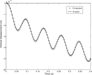
Figure 8. Terzaghi dynamic consolidation: computed solution compared with the analytic solution given in [27].

where $a=(n^{(s)2}\rho^{(f)}+n^{(f)2}\rho^{(s)})/c$, $b=n^{(f)2}k_{c}/c$, $c=(\lambda^{(s)}+2\mu^{(s)})n^{(f)2}$, $k_{c}=1\times 10^{6}$, $I_{0}(z)$ is the modified Bessel function of zeroth order, and $U(t)$ is a unit Heaviside function. The computed solution using the proposed quasi-static model is shown in Figure 8. Notice that the model performs well even though the loading is nonlinear and the dynamic response of the solid is treated in a quasi-static fashion.

5.3. Surface subsidence problem

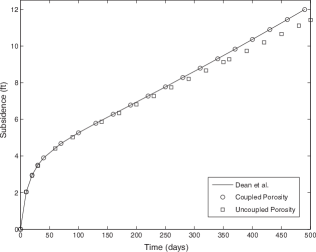
Figure 10. Surface subsidence: Comparison of the subsidence at the center of the top of the domain with published results in [29] for both coupled and uncoupled porosity.

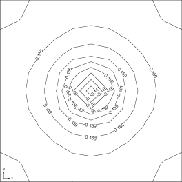
Figure 11. Surface subsidence: Contours of porosity for the top surface of the domain.

In this verification problem we consider the subsidence of a reservoir resulting from extraction of fluid via a centrally located well that has been studied extensively in [29]. Figure 9 shows the domain and boundary conditions used for this problem. In order to create confinement conditions similar to the subsurface environment an initial stress state was specified for the solid stress. The coupling between the solid stress and the fluid pore pressure is defined by equation (39) and the porosity model corresponds to equation (40f). The quasi-static model given in the previous examples was also used for the governing equations. Figure 10 shows a comparison between the results published in [29] and the computed results from the present study. Results are shown for both coupled and uncoupled porosity. Close correlation is achieved for the subsidence of the center of the top surface the domain for the coupled results. If the effect of the solid deformation is not taken into account in the porosity, the subsidence of the top surface is under-predicted by roughly 5%. Figure 11 shows contours of porosity for the top surface of the domain. Notice that near the ejection well, the porosity is decreased by almost 30% from the initial value.

5.4. Two-phase immiscible water flood

In the last example we present results for a water flood of the five spot well domain. The problem domain consists of two-dimensional square with injection wells at one of the sets of opposing corners and ejection wells at the other. Water is injected into the domain pushing oil out the ejection wells. The solution to this problem has been published for a number of numerical approaches including the results found in [30].

5.4.1. Changes in porosity vs. change in permeability due to solid stress

In the present study we consider the effects of both changes in porosity due to stresses in the solid skeleton and resulting changes in permeability due to damage. Conceptually, it is well established that solid deformation dependent porosity models behave like compressibility models. The otherwise incompressible fluid is able to be squeezed into pores that are expanding and vice versa. This is also apparent from the solid stress dependent contribution to the fluid equations showing up in the mass balance equation. In addition to the effect of pores enlarging and collapsing, one may wish to incorporate the increased permeability or interconnectedness of the void spaces due to solid damage. For example, in regions of high stress in the reservoir rock, cracks will form that allow fluid to flow with much less resistance. As a result, the flow magnitude and path of the fluid may change depending on the state of stress in the geologic formation. To explore differences between porosity coupled and permeability coupled models we investigate the two-phase water flood problem using both models separately. For the porosity coupled results we employ the model given in equation (40f), for the permeability coupled results we consider a damage modified permeability model given as:

$$\alpha^{(f)}=\alpha^{(f)}_{0}\left(1.0+\frac{\zeta||\boldsymbol{T}^{(s)}-\boldsymbol{T}_{0}^{(s)}||}{||\boldsymbol{T}_{0}^{(s)}||}\right)$$ (49)

where $\zeta$ is a scaling parameter. The permeability coupled model is based on the magnitude of the solid stress tensor, $||\boldsymbol{T}^{(s)}||$ normalized by the tensor magnitude of the stress in the solid due to in-situ conditions, $||\boldsymbol{T}_{0}^{(s)}||$. This ad-hoc model will serve as the basis for comparison with the coupled porosity model. In a forthcoming work, we investigate damage modified permeability models more thoroughly.

Since we are dealing with two-phase immiscible flow, we modify the governing equations of the quasi-static model as follows:

$$\frac{\partial}{\partial t}(\rho_{w}^{(f)}\phi(1-S_{n}))+\mathrm{div}[\rho_{w}^{(f)}\boldsymbol{v}_{w}^{(f)}] =m_{w}^{(f)}\quad\mbox{in}\;\Omega$$ (50a)

$$\frac{\partial}{\partial t}(\rho_{n}^{(f)}\phi S_{n})+\mathrm{div}[\rho_{n}^{(f)}\boldsymbol{v}_{n}^{(f)}] =m_{n}^{(f)}\quad\mbox{in}\;\Omega$$ (50b)

$$\mathrm{div}[\boldsymbol{T}^{(s)}] =0\quad\mbox{in}\;\Omega$$ (50c)

$$p^{(f)}(\boldsymbol{x}) =p^{\mathrm{p}}(\boldsymbol{x})\quad\mbox{on}\;\Gamma^{p}$$ (50d)

$$\boldsymbol{u}^{(f)}(\boldsymbol{x}) =\boldsymbol{u}^{\mathrm{p}}(\boldsymbol{x})\quad\mbox{on}\;\Gamma^{\boldsymbol{u}}$$ (50e)

$$\boldsymbol{T}^{(s)}\boldsymbol{n} =\boldsymbol{t}^{\boldsymbol{n}}\quad\mbox{on}\;\Gamma^{\boldsymbol{t}}$$ (50f)

where $S$ is the saturation and the subscripts “$w$” and “$n$” denote the wetting and non-wetting phases respectively. Note that we have incorporated the relationship $S_{n}+S_{w}=1.0$ in the first equation. The Darcy velocities for this problem are given as:

$$\boldsymbol{v}_{w}^{(f)}=-\alpha^{(f)}(\mathrm{grad}[p_{w}^{(f)}]+\rho_{w}^{(f)}\boldsymbol{b}_{w}^{(f)})$$ (51)

$$\boldsymbol{v}_{n}^{(f)}=-\alpha^{(f)}(\mathrm{grad}[p_{n}^{(f)}]+\rho_{n}^{(f)}\boldsymbol{b}_{n}^{(f)})$$ (52)

Here we have assumed no capillary pressure such that $p_{n}=p_{w}$. With this assumption, the equations above may be solved for $S_{n}$ and $p_{n}$ (or $p_{w}$). Note that we are using the same damage modified permeability $\alpha^{(f)}$ for both phases. To limit the spurious oscillations engendered by the advection terms, we use the CVFEM upwinding method presented by Forsyth in references [31, 32].

The problem domain and boundary conditions are shown in Figure 12. The elastic properties for the reservoir (used only in the coupled results) were generated by the code Sierra/Encore [33, 34] using a Karhunen–Loéve realization. Contours of $\lambda^{(s)}$ are shown in Figure 13. Notice large regions of variation of the elastic properties throughout the domain. Also shown in Figure 13 are contours of the porosity and permeability at time $t=2\times 10^{8}\;\mathrm{s}$ for both porosity coupled and permeability coupled results. Figure 14 shows the tensor magnitude contours of the solid stress due to the pore pressure loading. When compared with Figure 13 it reveals that the porosity model exhibits its largest porosity in a concentrated region near the region of low solid stress magnitude. The permeability model on the other hand shows high permeability in regions of high stress as the model intends. This results in a drastically different flow behavior between the models as shown in Figure 15. The top-left side of Figure 15 shows the non-wetting phase saturation for uncoupled two phase model. The top-right part of the figure shows the non-wetting phase saturation for the porosity coupled model. Notice that the differences with the uncoupled model are negligible. In contrast, the damage modified permeability model results clear show race-tracking in the regions of high stress, which is shown the bottom side of Figure 15. This example highlights the need for further model development to capture damage motivated permeability effects.

6. CONCLUDING REMARKS

We have considered a comprehensive mathematical model for flow of an incompressible fluid in deformable porous solid. The model is based on the theory of interacting continua with deformation-dependent porosity and damage modified permeability. The model also takes into account the dependence of viscosity the fluid on the pressure of the fluid. The model is fully coupled in the sense that the flow problem depends on the response of the porous solid, and the deformation of the porous solid depends on the velocity of the fluid. Several numerical coupling algorithms to obtain coupled flow-deformation response are also presented. Representative numerical results show the importance of considering the deformation of the solid on the flow and vice-versa. A possible future work is develop models and numerical coupling algorithms for flow in an elasto-plastic fracturable porous solid.

Figure 7. Terzaghi dynamic consolidation: problem geometry and boundary conditions

Figure 9. Surface subsidence: Problem geometry, parameters, and boundary conditions.

Figure 12. Two phase immiscible water flood: Problem geometry, parameters, and boundary conditions.

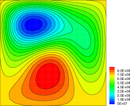
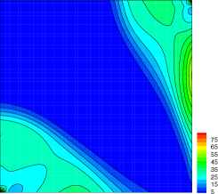
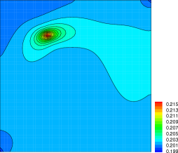
Figure 13. Two phase immiscible water flood: Contours of $\lambda^{(s)}$ (top-left), $\alpha$ (top-right), and $\phi$ (bottom).

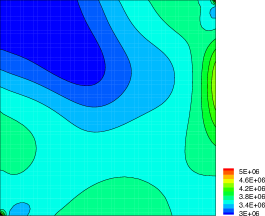
Figure 14. Two phase immiscible water flood: solid stress magnitude.

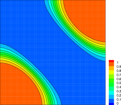
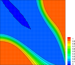
Figure 15. Two phase immiscible water flood: Contours of $S_{n}$. The top-left figure shows the non-wetting phase saturation for uncoupled two phase model. The top-right figure shows the non-wetting phase saturation for the porosity coupled model. The bottom figure shows the non-wetting phase saturation obtained using the damage modified permeability model. There are no noticeable differences between the results between the uncoupled model and the porosity coupled model. In contrast, the damage modified permeability model results clear show race-tracking in the regions of high stress.

References

- [1] A. Leach, C. F. Mason, and K. Veld. Co-optimization of enhanced oil recovery and carbon sequestration. Technical Report NBER Working Paper No. 15035, National Bureau of Economic Research, 2009.
- [2] A. M. Macfarlance. Energy: The issue of the century. Elements, 3:165–170, 2007.
- [3] D. P. Schrag. Confronting the climate-energy challenge. Elements, 3:171–178, 2007.
- [4] S. Bachu. Screening and ranking of sedimentary basins for sequestration of in geological media in response to climate change. Environmental Geology, 44:277–289, 2003.
- [5] S. M. Benson and D. R. Cole. sequestration in deep sedimentary formations. Elements, 4:325–331, 2008.
- [6] H. Darcy. Les Fontaines Publiques de la Ville de Dijon. Victor Dalmont, Paris, 1856.
- [7] P. Bobeck. The Public Fountains of the City of Dijon. Kendall Hunt Publishing, Dubuque, Iowa, USA, 2004.
- [8] A. Fick. Über diffusion. Poggendorff’s Annalen der Physik und Chemie, 94:59–86, 1855.
- [9] C. Truesdell. Sulla basi della thermomechanica. Rendiconti dei Lincei, 22:33–38, 1957.
- [10] C. Truesdell. Sulla basi della thermomechanica. Rendiconti dei Lincei, 22:158–166, 1957.
- [11] C. Truesdell and R. A. Toupin. The Classical Field Theories in Handbuch der Physik, volume III/1, pages 226–793. Springer-Verlag, New York, 1960.
- [12] C. Truesdell. Rational Thermodynamics. Springer, New York, USA, 1984.
- [13] R. J. Atkin and R. E. Craine. Continuum theories of mixtures: Basic theory and historical development. The Quaterly Journal of Mechanics and Applied Mathematics, 29:209–244, 1976.
- [14] R. M. Bowen. Theory of mixtures. In A. C. Eringen, editor, Continuum Physics, volume III. Academic Press, New York, 1976.
- [15] A. Bedford and D. S. Drumheller. Theories of immiscible and structured mixtures. International Journal of Engineering Science, 21:863–960, 1983.
- [16] R. Bowen. Porous Elasticity: Lectures on the Elasticity of Porous Materials as an Application of the Theory of Mixtures. Available online: http://repository.tamu.edu/handle/1969.1/2500, Texas A&M University, 2010.
- [17] O. Coussy. Poromechanics. John Wiley & Sons, Inc., New York, USA, 2004.
- [18] O. Coussy. Mechanics and Physics of Porous Solids. John Wiley & Sons, Inc., New York, USA, 2010.
- [19] R. de Boer. Theory of Porous Media: Highlights in the Historical Development and Current State. Springer-Verlag, New York, USA, 2000.
- [20] K. R. Rajagopal and L. Tao. Mechanics of Mixtures. World Scientific Publishing, River Edge, New Jersey, USA, 1995.
- [21] G. Z. Voyiadjis and C. R. Song. The Coupled Theory of Mixtures in Geomechanics with Applications. Springer-Verlag, New York, USA, 2006.
- [22] C. Barus. Isotherms, isopiestics and isometrics relative to viscosity. American Journal of Science, 45:87–96, 1893.
- [23] K. B. Nakshatrala and K. R. Rajagopal. A numerical study of fluids with pressure dependent viscosity flowing through a rigid porous medium. International Journal for Numerical Methods in Fluids, 67:342–368, 2011.
- [24] P. W. Bridgman. The Physics of High Pressure. MacMillan Company, New York, USA, 1931.
- [25] H. C. Brinkman. A calculation of the viscous force exerted by a flowing fluid on a dense swarm of particles. Applied Scientific Research, A1:27–34, 1947.
- [26] P. D. Lax. Functional Analysis. John Wiley & Sons, Inc., New York, USA, 2002.
- [27] R. de Boer, W. Ehlers, and Z. Liu. One-dimensional transient wave propagation in fluid-saturated incompressible porous media. Applied Mechanics, 63:59–72, 1993.
- [28] S. Diebels and W. Ehlers. Dynamic analysis of a fully saturated porous medium accounting for geometrical and material non-linearities. International Journal for Numerical Methods in Engineering, 39:81–97, 1996.
- [29] R. H. Dean, X. Gai, C. M. Stone, and S. E. Minkoff. A comparison of techniques for coupling porous flow and geomechanics. Society of Petroleum Engineers, SPE 79709:132–140, 2003.
- [30] R. Helmig. Multiphase Flow and Transport Processes in the Subsurface: A Contribution to the Modeling of Hydrosystems. Springer-Verlag, Berlin, second edition, 1997.
- [31] P. Forsyth. A control-volume, finite-element method for local mesh refinement in thermal reservoir simulation. SPE Reservoir Engineering, 5:561–566, 1990.
- [32] P. Forsyth. A control volume finite element approach to NAPL groundwater contamination. SIAM Journal on Scientific and Statistical Computing, 12:1029–1057, 1991.
- [33] P. Notz, S. R. Subia, M. Hopkins, H. K. Moffat, and D. R. Noble. Aria 1.5 User Manual. Technical report, Sandia Report SAND2007-2734, Sandia National Laboratories, 2007.
- [34] Fuego. SIERRA/Fuego 2.7 User’s Manual. Sandia National Laboratories, SAND 2006-6084P, 2008.