DYSON–SCHWINGER APPROACH TO STRONGLY COUPLED THEORIES

Abstract

Although nonperturbative functional methods are often associated with low energy Quantum Chromodynamics, contemporary studies indicate that they provide reliable tools to characterize a much wider spectrum of strongly interacting many-body systems. In this review, we aim to provide a modest overview on a few notable applications of Dyson–Schwinger equations to QCD and condensed matter physics. After a short introduction, we lay out some formal considerations and proceed by addressing the confinement problem. We discuss in some detail the heavy quark limit of Coulomb gauge QCD, in particular the simple connection between the nonperturbative Green’s functions of Yang–Mills theory and the confinement potential. Landau gauge results on the infrared Yang–Mills propagators are also briefly reviewed. We then focus on less common applications, in graphene and high-temperature superconductivity. We discuss recent developments, and present theoretical predictions that are supported by experimental findings.

Received (Day Month Year)Revised (Day Month Year)

PACS Nos.: 71.10.-w,12.38.Aw,72.80.Vp

1 Introduction

Quite generally, one of the challenges of modern theoretical physics is to explain the dynamics of quantum systems. Among them, fermion-fermion interactions are very specific and generate a large number of effects — from quark confinement in hadron physics, to quark gluon plasma in heavy ion collisions, from superconductivity in metals to band structure in crystals. Many different methods have been devised to tackle the many-body problem, under a variety of circumstances and at different energy scales. In high energy QCD, where asymptotic freedom guarantees that the coupling between quarks and gluons can be treated as a small parameter, perturbation theory has been successfully applied. At intermediate and low momenta, different methods are required since the coupling increases as we go to lower energies and perturbation theory alone cannot give a good description of the theory. One possibility is to employ continuum functional techniques such as renormalization group[1] and Dyson–Schwinger equations.[2, 3] Alternatively, numerical lattice simulations represent a potentially exact method, however extrapolation to chiral and infinite volume limits is often a numerical challenge.[4, 5] The situation is very similar in condensed matter electronic systems, where an equivalent program has been implemented.[6, 7, 8, 9]

This review is organized as follows. In section 2 we briefly review the general features of Dyson–Schwinger equations, and proceed in section 3 by discussing the confinement problem, with particular emphasis on the heavy quark limit of Coulomb gauge QCD. A brief overview of the progress made on infrared propagators of Landau gauge Yang–Mills theory is also attempted. Phenomenological findings are not discussed here, since they have been presented in many other works, see for example Ref. Roberts:2012sv for a recent review. In section 4 we turn to planar condensed matter systems. We exemplify the Dyson–Schwinger approach to strongly interacting many electron systems with two case studies, graphene and high temperature superconductors (HTSs). Our choice is motivated by the fact that these systems share a common aspect, namely, they can be described by effective quantum field theoretical models that inherit features of both (2+1) dimensional Quantum Electrodynamics (QED₃) and its four dimensional counterpart. We present results obtained from the Dyson–Schwinger equations, and where available the supporting experimental evidences. At the more formal level, it is also worth mentioning the similarities between the propagators of Yang–Mills theory and QED₃, i.e., the possibility of power law behavior in the deep infrared. A short summary is presented in section 5.

2 Dyson–Schwinger formalism

Dyson–Schwinger equations built up an infinite set of coupled non-linear integral equations that relate the various Green’s functions of a quantum field theory. From a practical point of view, defining a tractable problem requires the ability to reduce these equations to a closed subset, e.g. by making controlled ansätze for the higher order Green’s functions. In general the resulting coupled integral equations are solved numerically, nevertheless it is possible that in particular setups, such as heavy quark sector of Coulomb gauge QCD (under certain truncations), or infrared limit of Landau gauge Yang–Mills theory, exact analytic solutions become available. These aspects will be discussed in more detail in the next section.

The derivation of the Dyson–Schwinger equations rests on the idea that the generating functional of a theory

$$Z[J]=\int{\cal D}\Phi\exp{\left\{\mathrm{i}{\cal S}+\mathrm{i}{\cal S}_{s}\right\}}$$ (2.1)

is invariant under the variation of a generic field $\Phi_{\alpha}$:

$$\int{\cal D}\Phi\frac{\delta}{\delta\mathrm{i}\Phi_{\alpha}}\exp\left\{\mathrm{i}{\cal S}+\mathrm{i}{\cal S}_{s}\right\}=0,$$ (2.2)

where ${\cal S}$ is the action of the problem at hand, ${\cal S}_{s}$ the corresponding source term and ${\cal D}\Phi$ denotes the integration over all fields. To ensure the validity of this equation, translational invariance of the measure ${\cal D}\Phi$ is assumed. From Eq. (2.2), one can derive the Dyson–Schwinger equation for any $n$-point Green’s function, by taking further functional derivatives with respect to the fields and omitting those terms which vanish when the sources are set to zero.

Among the most investigated Dyson–Schwinger equations is the fermion gap equation, which, regardless of the underlying gauge theory, has the diagrammatical representation shown in Fig. 1. It essentially states that the inverse of the nonperturbative fermion propagator equals the sum between the inverse of the bare fermion propagator and the fermion self energy, which in turn contains dressed fermion and gauge boson propagators, and one bare and one dressed fermion-gauge boson vertex. Formally, the fermion gap equation appears in systems as discrepant as QCD, graphene and superconductors, whereby the raw form Fig. 1 has to be customized to the particular theory under consideration.

In addition to formal analogies, there are also important qualitative similarities between the systems that we are going to examine. An example is the possibility of scaling laws for the propagators in the deep infrared — a feature shared by both Landau gauge Yang–Mills theory and QED₃ (including high temperature superconductors, which can be described with a model that has properties reminiscent of QED₃). [3, 11, 12]

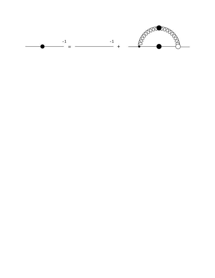
Figure 1: Dyson–Schwinger equation for a generic fermion propagator in a gauge theory. Filled circles denote dressed propagators, the empty circle denotes the dressed fermion-gauge boson vertex, the spring denotes the gauge propagator and solid lines stand for the fermion propagator.

3 Confining solutions from the Dyson–Schwinger equations

Confinement, i.e., the experimental evidence that quarks and gluons must be confined into color singlet hadronic states, represents, along with chiral symmetry breaking, one of the theoretical pillars of low energy hadron physics. A rigorous understanding of this phenomenon, i.e., identifying the specific mechanisms that act at the level of the underlying (gauge dependent) Green’s functions, is to date still an open problem.

As is well known, in order to overcome the difficulties related to the definition of the generating functional Eq. (2.1), the QCD action needs to be supplemented by a gauge fixing term, along with the associated ghost fields. Among various options, Coulomb gauge $\partial_{i}A_{i}^{a}=0$ has properties that qualify it as an efficient choice to study nonperturbative phenomena: in this gauge, Gauss law is naturally built in such that gauge invariance is fully accounted for, the total color charge is conserved and vanishing,[13, 14] and most importantly, a natural picture of confinement emerges. Furthermore, Coulomb gauge allows for different manifestations of confinement depending on the specific formalism, as shall be discussed below.

In the Hamiltonian formalism, Coulomb gauge is implemented simultaneously with Weyl gauge $A_{0}=0$.[15, 16, 17, 18, 19] In this approach, the Dyson–Schwinger equations for the ghost and spatial gluon propagators have been solved, analytically in the infrared and numerically in the whole momentum regime [16, 17, 20, 21, 22] (in Ref. Reinhardt:2011hq recent results at finite temperature are presented). Similar to Landau gauge scaling solutions,[24, 25, 26] the ghost and gluon dressing functions exhibit power law behaviors, $(p^{2})^{\delta_{gh}}$ and $(p^{2})^{\delta_{gl}}$. A general infrared power law analysis has yielded the following relation between the infrared exponents (with Landau and Coulomb gauge differing only in the number of dimensions $d$) [27, 20]

$$\delta_{gl}+2\delta_{gh}=\frac{4-d}{2}.$$ (3.3)

In the case $d=3$, which corresponds to equal-time Green’s functions in Coulomb gauge, two power law exponents $\kappa:=-\delta_{gh}$ have been found, $\kappa^{(1)}=0.398$ and $\kappa^{(2)}=1/2$ [20]. The energetically favored solution is the most singular, which produces a ghost propagator dressing function diverging as $1/|\vec{k}|$. In turn, this gives rise to a strictly linearly rising static quark potential at large distances.[21] The case $d=4$ trivially leads to the Landau gauge scaling relation $\delta_{gh}=-\delta_{gl}/2$ [27, 26] (see also the discussion at the end of this section).

In the functional formalism (as applied to Coulomb gauge QCD), apart from the ghost and transversal spatial gluon propagator, there is a third propagator, the temporal gluon propagator, which plays an important role in uncovering the confining potential between (static) quarks. To see how this comes about, let us first briefly review the main characteristics of the functional formalism.

In general, functional Dyson–Schwinger studies in Coulomb gauge are plagued by the so-called energy divergence problem, i.e., the unregulated divergences generated by ghost loops, as in the one-loop integral $\int dk_{0}\int d^{3}\vec{k}[(\vec{k}-\vec{p})^{2}\vec{k}^{2}]^{-1}$. The usual dimensional regularization fails in this case, although the full set of such loops should cancel in the Dyson–Schwinger equations. While such cancellations have been isolated up to two loops in perturbation theory,[28, 29, 30, 31] they are exceedingly difficult to pin down in the full tower of Dyson–Schwinger equations. This problem can be bypassed by converting to first order functional formalism, i.e., linearizing the chromoelectric term in the action via the auxiliary field $\vec{\pi}$ [13]

$$\exp{\left\{\mathrm{i}\int d^{4}x\frac{1}{2}{\vec{E}}\!\cdot\!{\vec{E}}\right\}}=\int{\cal D}\vec{\pi}\exp{\left\{\mathrm{i}\int d^{4}x\left[-\frac{1}{2}{\vec{\pi}}\!\cdot\!{\vec{\pi}}-{\vec{\pi}}\!\cdot\!{\vec{E}}\right]\right\}}.$$ (3.4)

The $\vec{\pi}$ field is subsequently split into transverse and longitudinal components (details are provided in Ref. Watson:2006yq). With this new fields, the QCD action is rewritten such that the ghost field, i.e., the Faddeev-Popov determinant, cancels against the inverse functional determinant that stems from resolving the chromodynamical equivalent of the Gauss law. The resulting action contains only the ’would-be-physical’ degrees of freedom, the transverse $\vec{A}$ and $\vec{\pi}$ fields (which classically would correspond to the configuration variables and their momentum conjugates), whereas the unphysical ghosts are formally eliminated. The shortcoming, however, is that we end up with a nonlocal Lagrangian that is unsuited for practical applications.[13, 32] Nevertheless, the nonlocal formulation can provide important guidelines to the local theory.

It is important to realize that identifying the mechanisms that lead to the cancellations of the unphysical components is essential for a thorough understanding of the theory. For example, the (unphysical) energy-independent ghost loop mentioned above should be canceled by the temporal component of the gluon propagator, and this implies that the temporal gluon itself must have an energy-independent part.[33] This argument is supported by lattice results [34] and analytic findings [35]. In the limit of the heavy quark mass, this information has been used as input to derive a relation between the temporal gluon propagator and the nonperturbative scale associated with confinement (the string tension).[36] We will return to this relation below.

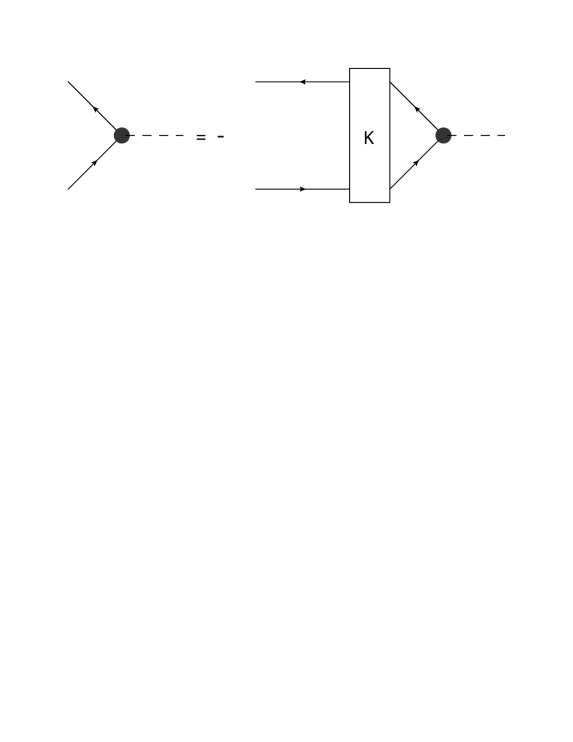
Figure 2: Homogeneous Bethe–Salpeter equation for quark-antiquark bound states. Solid lines represent the (dressed) quark propagators, dashed lines denote the corresponding bound state, and blobs denote the Bethe–Salpeter vertex function. The box represents the Bethe–Salpeter kernel which in the heavy quark limit reduces to the exchange of a single temporal gluon.

Explicitly, heavy quark limit refers in this case to a heavy quark mass expansion of the QCD action at leading order, with the truncation of the Yang–Mills sector to include only dressed propagators. In this framework, a full nonperturbative study of the gap and Bethe–Salpeter equations has been performed. Solving the gap equation (generically represented in Fig. 1) yields the following solution for the heavy quark propagator:

$$W_{\overline{q}q}(k_{0})=\frac{-\mathrm{i}}{\left[k_{0}-m-{\cal I}_{r}+\mathrm{i}\varepsilon\right]},$$ (3.5)

where $m$ denotes the quark mass and ${\cal I}_{r}$ is an (implicitly regularized) constant. Since this propagator has a single pole in the complex $k_{0}$ plane, it follows that the closed quark loops are suppressed, and this implies that the theory is quenched in the heavy mass limit:

$$\int dk_{0}\frac{1}{\left[k_{0}-m-{\cal I}_{r}+\mathrm{i}\varepsilon\right]\left[k_{0}+p_{0}-m-{\cal I}_{r}+\mathrm{i}\varepsilon\right]}=0.$$ (3.6)

By using the associated Slavnov–Taylor identity, it is easy to show that the temporal quark-gluon vertex remains nonperturbatively bare, $\Gamma_{\bar{q}qA_{0}}\to\Gamma_{\bar{q}qA_{0}}^{(0)}=gT^{a}$, with $T^{a}$ being the hermitian generators of the gauge group. Moreover, the kernel of the Bethe–Salpeter equation, depicted in Fig. 2, reduces to a single gluon exchange:

$$K(k)=\Gamma^{a}_{\bar{q}qA_{0}}\,W_{00}^{ab}(\vec{k})\,\Gamma^{Tb}_{q\bar{q}A_{0}},$$ (3.7)

where $W_{00}(\vec{k})$ is the temporal gluon propagator (a complete description and derivation is provided in Ref. Popovici:2010mb). With the kernel Eq. (3.7), the bound state energy between a quark and an antiquark at leading order in the mass expansion reads:

$$P_{\bar{q}q}=g^{2}\int_{r}\frac{d\vec{\omega}}{(2\pi)^{3}}W_{00}(\vec{\omega})\left[C_{F}-C_{M}e^{\mathrm{i}\vec{\omega}\cdot\vec{x}}\right],$$ (3.8)

where the index ’$r$’ denotes an implicitly regularized integral, $C_{F}$ is the Casimir factor, $C_{M}$ denotes an (unknown) color factor assigned to the quark-meson vertex, and $|\vec{x}|$ represents the separation between the quark and the antiquark. To identify $C_{M}$, we recall that since a quark cannot live as asymptotic state,[14] the bound state energy $P_{\bar{q}q}$ must be linearly rising, or otherwise the energy is infinite and the quark-antiquark system is not allowed. With a temporal gluon dressing function more divergent than $1/|\vec{\omega}|$, it follows that $C_{M}=C_{F}$ and hence a finite solution of the Bethe–Salpeter equation exists only for color singlet states. Assuming that in the infrared

$$W_{00}(\vec{\omega})=\frac{X}{\vec{\omega}^{4}},$$ (3.9)

where $X$ is a combination of constants (and $g^{2}X$ is a renormalization group invariant [13]), Eq. (3.8) reduces to

$$P_{\bar{q}q}:=\sigma|\vec{x}|=\frac{g^{2}C_{F}X}{8\pi}|\vec{x}|.$$ (3.10)

This result provides the link (at least at leading order) between the physical string tension $\sigma$ and the nonperturbative Yang–Mills sector of QCD. It corresponds to the only physical solution (a color singlet bound state of a quark and an antiquark) or else the energy of the system is divergent. A similar calculation performed for the diquark Bethe–Salpeter equation has shown that diquarks are confined for $N_{c}=2$ colors, which corresponds to a confined, antisymmetric bound state of two quarks (the $SU(2)$ baryon), and otherwise there are no physical states. Finally, a thorough investigation of the Dyson–Schwinger equation for the full nonperturbative four-point quark-antiquark Green’s functions has evidenced the separation of the physical and unphysical singularities of the Green’s function, and that the physical pole coincides with the pole Eq. (3.8) of the homogenous Bethe–Salpeter equation.[41] An analogous investigation for the diquark system has shown that the resonant pole of the four-point Green’s function is attached to the only physical solution, for $N_{c}=2$ colors, corresponding to color antisymmetric and flavor symmetric configuration.

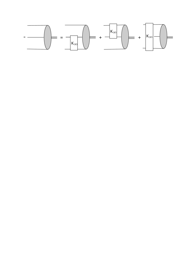
Figure 3: Faddeev equation for three-quark bound states. The box depicts in this case the diquark kernel, the ellipse denotes the Faddeev vertex function, and the triple lines represent the three-quark bound state. Same conventions as in Fig. 2 apply.

Following the same approach, a similar analysis has been carried out for three quark systems by means of Faddeev equation, depicted in Fig. 3.[42] Since in the quark-diquark model the binding energy between quarks is assumed to be provided essentially by two-quark correlations,[43] in the Faddeev equation only the permuted two-quark kernels $K_{(d)}$ are employed, whereas the three-body irreducible diagrams are neglected. Just like for $\bar{q}q$ states, the diquark kernel reduces to the ladder approximation,

$$K_{(d)}(k)=\Gamma_{\bar{q}qA_{0}}^{a}\,W_{00}^{ab}(\vec{k})\,\Gamma_{\bar{q}qA_{0}}^{b}.$$ (3.11)

By working in the symmetric case (equal spatial separations between quarks), the following three-quark bound state energy has been determined as a solution of the Faddeev equation

$$P_{3q}=3m+\frac{3}{2}g^{2}\int_{r}\frac{d\vec{\omega}}{(2\pi)^{3}}W_{00}(\vec{\omega})\left[C_{F}-2C_{B}e^{\mathrm{i}\vec{\omega}\cdot\vec{x}}\right],$$ (3.12)

where $C_{B}$ denotes the color factor attached to the quark-baryon vertex. As before, the only possibilities are either that the $3q$ system is confined, or it is physically not allowed. An infrared confining solution requires that the condition $C_{B}=C_{F}/2$ is satisfied, provided that the temporal gluon propagator is infrared enhanced. This implies that the baryon is a color singlet bound state of three quarks and otherwise the energy of the system is infinite. Inserting $C_{B}=C_{F}/2$, along with the infrared temporal gluon propagator Eq. (3.9), into Eq. (3.12), yields the following result for the bound state energy of the three quark system:

$$P_{3q}=3m+\frac{3}{2}\frac{g^{2}C_{F}X}{8\pi}|\vec{x}|.$$ (3.13)

As in the case of $\bar{q}q$ systems, the ’string tension’, i.e., the coefficient of the three-body linear confinement term, is directly related to the nonperturbative temporal gluon propagator. Comparing the above result with Eq. (3.10), it appears that the string tension corresponding to the $qqq$ system is 3/2 times that of the $\bar{q}q$ system. The $3m$ term is a reminiscence of the heavy quark transformation which enters the Faddeev equation via the heavy quark propagator, Eq. (3.5).

Let us now turn our attention towards Landau gauge $\partial_{\mu}A_{\mu}^{a}=0$. Unlike Coulomb gauge, where one is faced with severe technical difficulties introduced by noncovariance, Landau gauge remains popular due to its covariance, but also because of certain technical simplifications (the ghost-gluon vertex remains approximately bare in the infrared [44]). In this gauge, the coupled system of Dyson–Schwinger equations for ghost and gluon propagators has been solved,[26, 45] see also the discussion above Eq. (3.3). It was found that the gluon propagator vanishes at zero momentum, whereas the ghost propagator is infrared enhanced, in agreement with the ghost dominance picture of Gribov and Zwanziger,[46, 47, 13] and Kugo and Ojima.[48, 49, 50] With the truncation to employ a bare ghost-gluon vertex, the scaling coefficient $\kappa\approx 0.595$ has been calculated independently in Refs. Zwanziger:2001kw and Lerche:2002ep. By combining informations stemming from both Dyson–Schwinger and renormalization group equations, it has been shown that the Landau gauge scaling solution is unique (however, this should not be confused with the uniqueness of the solution itself).[51]

On the lattice, it eventually become clear that the gluon propagator is not vanishing at small momentum; instead, a massive behavior has been seen, although some papers were still in agreement with a vanishing gluon propagator, see for example Ref. Vandersickel:2012tz and references therein. These findings support the so-called decoupling solution — a second solution derived with Dyson–Schwinger methods, where the gluon and ghost propagate quite differently: at small momenta, the gluon propagator becomes finite instead of going to zero, whereas the ghost dressing remains finite.[53, 54, 55] In order to understand the connection between the two solutions, it is necessary to examine the renormalization of the ghost propagator. A finite ghost dressing function at zero momentum generates a continuous set of decoupling solutions, whereas if an infinite ghost dressing at zero momentum is employed, the scaling solution is recovered.[56] Finally, we note that a numerical analysis of gluon and ghost propagators in the complex momentum plane has been recently carried out.[57]

Importantly, both the decoupling and scaling solutions fulfill the criterion for a confining Polyakov loop potential, meaning that quarks are confined.[58] This criterion depends only on the asymptotic part, and as it turns out, in the actual calculations the dynamics of the system is driven by the non-perturbative mid-momentum regime (where both solutions agree), and not the deep infrared.

4 Manifestations of (2+1) dimensional QED in condensed matter physics

Although when studying gauge theories it seems natural to consider a theory set in $3+1$ dimensions, it is nevertheless possible that some insight might be gained by restricting to $2+1$ dimensions. An example is QED₃, which apart from having intrinsically interesting features, such as superrenormalizability,[59] is also attractive for its ability to describe the behavior of certain materials that lay at the border between particle and condensed matter physics, such as graphene and high temperature superconductors. The quantum field theoretical modeling of these materials has provided a description of phenomena that are nonperturbative in essence, e.g. dynamical mass generation via chiral symmetry breaking.

Before turning our attention to condensed matter systems, we note that the infrared behavior of Landau gauge QED₃ propagators is given by power laws, just like the scaling solutions of Landau gauge Yang–Mills theory (see also the discussion from the previous section). The QED₃ power laws have been derived from an infrared analysis of the coupled system of fermion and photon Dyson–Schwinger equations.[11]

4.1 Graphene

Graphene is a monatomic layer of carbon atoms arranged on a honeycomb lattice.[60, 61, 62] Its remarkable electronic properties, such as unconventional quantum Hall effect,[63, 64] Klein tunneling [65, 66] or charge confinement,[67] qualify it as one of the most promising materials for future nanoscale devices. Its synthesis in 2004 [68, 69] was awarded the Nobel Prize in physics in 2010.

The fundamentally new characteristics of this system are theoretically explicable in terms of the low energy behavior of the charge carriers: instead of the familiar Schrödinger equation, the electrons in graphene are described by the relativistic Dirac equation for massless fermions.[70, 71] The resulting single particle dispersion relation is linear in the momentum, $E_{k}=\pm v_{F}|\vec{k}|$, where $v_{F}$ is the Fermi velocity (about $300$ times smaller than the speed of light) and $\vec{k}=(k_{x},k_{y})$ is the fermion momentum, measured relative to the inequivalent corners of the Brillouin zone.

From a technological point of view, graphene based nanoscale devices require the ability to control the so-called charge confinement, i.e., the clustering of electronic charge such that the Klein effect can be overcome.[67] Theoretically, a low energy effective model that is well suited to describe various disorder phenomena has been constructed by means of a chiral gauge theory.[72, 73] This has been supplemented by scalar and gauge fields that account for the self-interaction of the carbon background and the mean self-interaction of the Dirac fermions.[74] In this framework, charge confinement has been described by modeling one-dimensional defects, associated e.g. with chemical bonding of foreign atoms to carbon atoms, as potential barriers which break sublattice symmetry.[75]

The single-particle picture, however, changes quite dramatically if the long range Coulomb interaction is taken into account. Since fermions are confined to live in the plane, whereas the gauge bosons live in three spatial dimensions, one is confronted with the problem of coupling the two-dimensional current with a three-dimensional gauge potential. This difficulty is solved by integrating the usual photon propagator over the third momentum dimension (known as dimensional reduction), which leads to an atypical behavior of the gauge propagator, namely, it goes like $1/k$, instead of $1/k^{2}$. This anomalous gauge propagator induces the renormalization of the electron self-energy, which is not present in ordinary QED₃.

Various theoretical studies have predicted that Coulomb interaction may generate dynamically a finite mass gap, such that graphene undergoes a phase transition from semimetal to insulator above some critical coupling $\alpha_{c}$.[76, 77, 78, 8, 79] This possibility is motivated by the large value of the ’bare’ coupling $\alpha=e^{2}/\epsilon hv_{F}$ of graphene on a substrate with dielectric constant $\epsilon$ (for suspended graphene $\alpha_{0}=2.19$).

On the other hand, most recent experiments find no signature of an insulating phase in suspended graphene.[80, 81] Measurements indicate, however, that the real dispersion relation is logarithmic, instead of linear, near the neutrality point. This reshaping of the Dirac cones is caused by the charge-carrier density dependent renormalization of the Fermi velocity (induced by the Coulomb interaction). In fact, the running of the fermion velocity with the energy was already predicted in earlier renormalization group calculations,[82] where it was found that the Fermi velocity grows logarithmically without bound, until retardation effects become important enough to invalidate the instantaneous Coulomb approximation.

To analyze the problem of the gap generation, it is useful to inspect the Dyson–Schwinger equation for the fermion propagator Fig. 1. Following the usual procedure, this equation is converted into a system of coupled integral equations for the Fermi velocity dressing function $A(p)$ and the gap function $\Delta(p)$, which characterize the fermion propagator,

$$S(p)^{-1}=\gamma^{0}p_{0}-v_{F}A(p)\,\gamma^{i}p_{i}-\Delta(p).$$ (4.14)

At the critical coupling $\alpha_{c}$, where the phase transition should take place, the system is well described by bifurcation theory. Applying bifurcation theory amounts to linearizing the equations around the critical point, i.e., neglect quadratic and higher order terms. By using a one-loop photon propagator, it has been found that the function $A(p)$ is logarithmically divergent,[83] in agreement with the experimental evidences.[80] Explicitly, it reads ($g=\alpha N_{f}\pi/4$)

$$A(p)=1+\frac{2}{\pi^{2}N_{f}g}\left\{-\left[\pi-2g+c(g)(g^{2}-1)\right]\ln\frac{p}{\Lambda}+f(g)\right\},$$ (4.15)

where $c(g)$ and $f(g)$ are functions of the coupling, $N_{f}=2$ for monolayer graphene, and the physical cutoff $\Lambda$ is determined by the size of the graphene’s Brillouin zone. This result is then used in the bifurcation analysis of the gap equation, which around the critical point reduces to:

$$\Delta(p)=\frac{e^{2}}{v_{F}\varepsilon}\int\frac{d^{2}\vec{k}}{(2\pi)^{2}}\frac{1}{k\,|\vec{p}-\vec{k}|}\frac{\Delta(k)}{A(k)}J\left(\frac{k}{|\vec{p}-\vec{k}|}A(k),g\right).$$ (4.16)

In the above, $J$ is a piecewise function that includes the effects of the Fermi velocity dressing function. Importantly, for determining the critical coupling corresponding to the semimetal-insulator transition, not only the logarithmic but also the regular contributions to the function $A(p)$, i.e. the function $f(g)$, become significant.[83] For the critical coupling it is obtained $\alpha_{c}=2.85$, which is larger than the bare coupling of suspended graphene $\alpha_{0}=2.19$. These findings are in agreement with the experimental observations that suspended graphene does not undergo a phase transition.[80] Hence, it appears that the logarithmic renormalization of Fermi velocity strongly weakens the Coulomb interaction, favoring the persistence of the semimetal phase in suspended graphene.[83]

Despite the encouraging results, a complete understanding of the physical picture requires a full nonperturbative investigation, by including the Dyson–Schwinger equation for the gauge propagator. Since nonperturbative contributions to both photon propagator and vertex functions have led to significant corrections in ordinary QED₃, it is likely that including these effects will lead to further corrections of the critical coupling. Furthermore, a proper comparison of our value for the critical coupling with lattice calculations is impeded by the details of the cutoff procedure in the ultraviolet, as lattice simulations have been performed on both ’standard’ squared [8] and hexagonal (physical) [84] lattices. Finally, as well known from ordinary QED₃, finite volume effects may also play a role, see for example Ref. Goecke:2008zh and references therein.

When comparing to the experiment, one has to keep in mind that other type of terms, such as four-fermion contact interactions, may also become important and thus have to be included in the model Lagrangian, in addition to the long-range Coulomb interaction. First studies in this direction have already been undertaken in Refs. Gamayun:2009em,Mesterhazy:2012ei,Herbut:2009qb. Another important line of study is to explore the effects of a finite chemical potential on the Fermi velocity — experimentally this corresponds to a finite density of charge carriers, i.e., chemical doping. This problem is currently under investigation.[88]

4.2 High-temperature superconductivity

Due to their properties apparently incompatible with conventional metal physics, high-T_c cuprate superconductors can be regarded as another example of QED₃ ’in the lab’. A particularly striking feature is the pseudogap — a third phase that lays at the boundary between the nonsuperconducting (in this case, associated with the antiferromagnetic spin density wave) and superconducting phases.[89] The physics of the pseudogap phase is dominated by strong pairing fluctuations, as has been experimentally demonstrated by measuring the so-called Nernst signal.[90]

Describing the pseudogapped phase theoretically is a challenge due to the complications introduced by the scattering of the fermions off the vortices (topological defects), which are otherwise bounded in the superconducting phase.[91] A way to circumvent this problem has been put forward by Franz and Tesanović, who adopted an ’inverted’ paradigm and proposed to start from the ’conventional’ superconducting phase and try to find the mechanism that describes the transition to the normal state.[92] In this approach, the fermion field is gauge transformed to a new field which the authors call ’topological fermions’. The pseudogap phase of the topological fermions is then associated with the chiral symmetric QED₃, whereas the transition to the antiferromagnetic phase is indicated by the generation of a dynamical mass for the quasiparticles.[93, 92, 89, 94] The generation of such a mass term results from interactions of the fermionic quasiparticles with topological excitations described by the gauge fields of QED₃.

An open question is whether at zero temperature a pseudogap associated to the onset of antiferromagnetic spin density wave instability is formed in the first place, or if the system is driven directly into the antiferromagnetic phase. The answer lays in the critical number of ’flavors’ of fermions $N_{f}^{c}$ where the system undergoes a phase transition from the chirally broken into the chirally symmetric phase. This has to be compared with the physical number of flavors $N_{f}=2$, which denotes the number of low energy quasiparticles located at the four nodal points of the gap function, see for example Ref. Franz:2002qy for details. If $N_{f}^{c}<2$, the theory will first go through the pseudogap phase; if, on the other hand, $N_{f}^{c}>2$, the system is driven directly from the superconducting into the antiferromagnetic phase upon further underdoping.

Furthermore, since experimental observations suggest that most of the HTS materials are strongly anisotropic due to the large difference between the Fermi velocity and a second velocity $v_{\Delta}$ (related to the amplitude of the superconducting order parameter),[95, 96] a complete theoretical description requires taking into account this intrinsic anisotropy as well. At the level of the Lagrangian, including the anisotropy amounts to implementing a nontrivial metric that collects the anisotropic fermion velocities.[12]

Much work has been devoted to determining the critical number of flavors $N_{f}^{c}$ at which chiral symmetry is broken, in the isotropic [97, 98, 99, 11] as well as anisotropic [93, 89, 100, 12] versions of QED₃. Studies carried out for isotropic QED₃ indicate that $N_{f}^{c}$ lays around $3.5-4$. In the following, we concentrate on anisotropic QED₃, and briefly review the results obtained within the Dyson–Schwinger formalism. In a first study, the Dyson–Schwinger equation for the fermion propagator has been solved in the limit of small anisotropic velocities.[93] It has been found that in this case there should be essentially no difference between the universal behavior of isotropic and anisotropic QED₃. Later on, a more sophisticated fermion dressing has been included, and again only the case of small anisotropic velocities has been considered.[89, 100] In the large-$N_{f}$ limit, it has been found that the critical number of flavors where the theory suffers the chiral phase transition stays the same. In a subsequent study,[101] a quantitative criterion that relates the critical number of fermion flavors and the strength of the photon-fermion coupling has been proposed, namely, it was conjectured that the dynamical fermion mass will be generated as soon the gauge field strength is larger than some threshold value which can be determined from the S-matrix for fermion-fermion scattering. It was concluded that velocity anisotropy does affect the number of critical fermion flavors at which chiral symmetry is broken due to mass generation. A recent reexamination of the situation going beyond the small anisotropy expansion, and using a power law ansatz for the photon propagator, has shown sizable deviations of the critical number of flavors from the isotropic case,[12, 102] in agreement with lattice results.[103, 104]

5 Summary

In this brief review we have presented a few selected applications of Dyson–Schwinger approach to strongly interacting fermion systems. In the first part we have considered the confinement problem, concentrating on the heavy quark limit of Coulomb gauge QCD. With the truncation to include only dressed Yang–Mills propagators, we have sketched the derivation of a simple relation between the Green’s functions of Coulomb gauge Yang–Mills theory and the quark confinement potential, for quark-antiquark and three-quark systems. Confining (finite energy) solutions exist only for color singlet meson/baryon states, and otherwise the systems have infinite energy. Further, we have seen that in the heavy quark limit, the rainbow approximation to the quark gap equation and the ladder approximation to the associated Bethe–Salpeter and Faddeev equations remain nonperturbatively exact. In the remainder of this part we have briefly reviewed Landau gauge results on the infrared Yang–Mills propagators.

In the second part we have moved on to less commonplace applications, in graphene and high temperature superconductors. These planar condensed matter systems are well described by effective QED₃-like theories, which are tailored to accommodate the particularities of the system under consideration. We have reviewed selected topics studied with Dyson–Schwinger methods, which include the problem of dynamical gap generation by long-range Coulomb interactions in suspended graphene, and the pseudogap phase in high temperature superconductors. In graphene, including renormalization effects on the Fermi velocity has lead to the conclusion that the Coulomb interaction is strongly weakened near the charge neutrality point, preventing the emergence of a gapped phase. These results agree with the experimental findings which indicate the persistence of the semimetal phase. In high-temperature superconductivity, where the physics of the pseudogap is strongly dependent on the number of fermion species, it has been shown that the inherent spatial anisotropy leads to a significant alteration of the critical number of flavors where the phase transition from chirally symmetric to chirally broken phase takes place (as compared to isotropic QED₃). Least but not last, it is important to appreciate the possible similarities between different theories, i.e., the scaling solutions of Landau gauge propagators of Yang–Mills theory and QED₃. In the context of high-T_c superconductivity, a power law ansatz for the photon propagator has been successfully employed to study the dynamical breaking of chiral symmetry. Whether the gauge field in graphene is characterized by a similar behavior remains to be clarified in the future.

References

- [1] J. M. Pawlowski, Annals Phys. 322 (2007) 2831–2915.
- [2] R. Alkofer and L. von Smekal, Phys.Rept. 353 (2001) 281.
- [3] C. S. Fischer, J. Phys. G32 (2006) R253–R291.
- [4] J. Greensite, Prog.Part.Nucl.Phys. 51 (2003) 1.
- [5] G. Colangelo, S. Durr, A. Juttner, L. Lellouch, H. Leutwyler, et al., Eur.Phys.J. C71 (2011) 1695.
- [6] P. W. Anderson, Basic notions of condensed matter physics, vol. 55 of Frontiers in Physics. The Benjamin/Cummings, 1984.
- [7] R. Shankar, Rev.Mod.Phys. 66 (1994) 129–192.
- [8] J. E. Drut and T. A. Lähde, Phys. Rev. B 79 (2009) 165425.
- [9] J. E. Drut and A. N. Nicholson, arXiv:1208.6556.
- [10] C. D. Roberts, arXiv:1203.5341.
- [11] C. S. Fischer, R. Alkofer, T. Dahm, and P. Maris, Phys. Rev. D 70 (2004) 073007.
- [12] J. A. Bonnet, C. S. Fischer, and R. Williams, Phys.Rev. B84 (2011) 024520.
- [13] D. Zwanziger, Nucl. Phys. B518 (1998) 237–272.
- [14] H. Reinhardt and P. Watson, Phys. Rev. D79 (2009) 045013.
- [15] C. Feuchter and H. Reinhardt, arXiv:hep-th/0402106.
- [16] C. Feuchter and H. Reinhardt, Phys. Rev. D70 (2004) 105021.
- [17] H. Reinhardt and C. Feuchter, Phys. Rev. D71 (2005) 105002.
- [18] A. P. Szczepaniak and E. S. Swanson, Phys. Rev. D65 (2002) 025012.
- [19] A. P. Szczepaniak and P. Krupinski, Phys.Rev. D73 (2006) 034022.
- [20] W. Schleifenbaum, M. Leder, and H. Reinhardt, Phys.Rev. D73 (2006) 125019.
- [21] D. Epple, H. Reinhardt, and W. Schleifenbaum, Phys. Rev. D75 (2007) 045011.
- [22] D. Epple, H. Reinhardt, W. Schleifenbaum, and A. P. Szczepaniak, Phys. Rev. D77 (2008) 085007.
- [23] H. Reinhardt, D. Campagnari, and A. Szczepaniak, Phys.Rev. D84 (2011) 045006.
- [24] L. von Smekal, R. Alkofer, and A. Hauck, Phys.Rev.Lett. 79 (1997) 3591–3594.
- [25] L. von Smekal, A. Hauck, and R. Alkofer, Annals Phys. 267 (1998) 1.
- [26] C. Lerche and L. von Smekal, Phys.Rev. D65 (2002) 125006.
- [27] D. Zwanziger, Phys.Rev. D65 (2002) 094039.
- [28] A. Andrasi and J. Taylor, Eur.Phys.J. C41 (2005) 377–380.
- [29] P. Watson and H. Reinhardt, Phys. Rev. D76 (2007) 125016.
- [30] G. Leibbrandt and J. Williams, Nucl.Phys. B475 (1996) 469–483.
- [31] G. Heinrich and G. Leibbrandt, Nucl.Phys. B575 (2000) 359–382.
- [32] P. Watson and H. Reinhardt, Phys. Rev. D75 (2007) 045021.
- [33] A. Cucchieri and D. Zwanziger, Phys. Rev. D65 (2001) 014002.
- [34] M. Quandt, G. Burgio, S. Chimchinda, and H. Reinhardt, PoS CONFINEMENT8 (2008) 066, arXiv:0812.3842.
- [35] P. Watson and H. Reinhardt, Phys.Rev. D82 (2010) 125010.
- [36] C. Popovici, P. Watson, and H. Reinhardt, Phys. Rev. D81 (2010) 105011.
- [37] M. Neubert, Phys. Rept. 245 (1994) 259–396.
- [38] P. Watson and H. Reinhardt, Phys.Rev. D85 (2012) 025014.
- [39] P. Watson and H. Reinhardt, Phys.Rev. D86 (2012) 125030.
- [40] C. Popovici, P. Watson, and H. Reinhardt, Phys. Rev. D79 (2009) 045006.
- [41] C. Popovici, P. Watson, and H. Reinhardt, Phys.Rev. D83 (2011) 125018.
- [42] C. Popovici, P. Watson, and H. Reinhardt, Phys.Rev. D83 (2011) 025013.
- [43] H. Reinhardt, Phys. Lett. B244 (1990) 316–326.
- [44] W. Schleifenbaum, A. Maas, J. Wambach, and R. Alkofer, Phys.Rev. D72 (2005) 014017.
- [45] C. Fischer and R. Alkofer, Phys.Lett. B536 (2002) 177–184.
- [46] V. N. Gribov, Nucl. Phys. B139 (1978) 1.
- [47] D. Zwanziger, Nucl. Phys. B485 (1997) 185–240.
- [48] T. Kugo and I. Ojima, Prog.Theor.Phys.Suppl. 66 (1979) 1.
- [49] T. Kugo, arXiv:hep-th/9511033.
- [50] P. Watson and R. Alkofer, Phys.Rev.Lett. 86 (2001) 5239.
- [51] C. S. Fischer and J. M. Pawlowski, Phys. Rev. D80 (2009) 025023.
- [52] N. Vandersickel and D. Zwanziger, Phys.Rept. 520 (2012) 175–251.
- [53] A. Aguilar, D. Binosi, and J. Papavassiliou, Phys.Rev. D78 (2008) 025010.
- [54] D. Dudal, S. Sorella, N. Vandersickel, and H. Verschelde, Phys.Rev. D77 (2008) 071501.
- [55] D. Dudal, J. A. Gracey, S. P. Sorella, N. Vandersickel, and H. Verschelde, Phys.Rev. D78 (2008) 065047.
- [56] C. S. Fischer, A. Maas, and J. M. Pawlowski, Annals Phys. 324 (2009) 2408–2437.
- [57] S. Strauss, C. S. Fischer, and C. Kellermann, Phys.Rev.Lett. 109 (2012) 252001.
- [58] J. Braun, H. Gies, and J. M. Pawlowski, Phys.Lett. B684 (2010) 262–267.
- [59] C. D. Roberts and A. G. Williams, Prog.Part.Nucl.Phys. 33 (1994) 477–575.
- [60] A. Castro Neto, F. Guinea, N. Peres, K. Novoselov, and A. Geim, Rev.Mod.Phys. 81 (2009) 109–162.
- [61] N. M. R. Peres, Reviews of Modern Physics 82 (2010) 2673–2700.
- [62] S. Das Sarma, S. Adam, E. H. Hwang, and E. Rossi, Reviews of Modern Physics 83 (2011) 407–470.
- [63] V. P. Gusynin and S. G. Sharapov, Physical Review Letters 95 (2005) 146801.
- [64] Y. Zhang, Y.-W. Tan, H. L. Stormer, and P. Kim, Nature 438 (2005) 201–204.
- [65] M. I. Katsnelson, K. S. Novoselov, and A. K. Geim, Nature Physics 2 (2006) 620–625.
- [66] V. V. Cheianov and V. I. Fal’Ko, Phys. Rev. B 74 (2006) 041403.
- [67] A. V. Rozhkov, G. Giavaras, Y. P. Bliokh, V. Freilikher, and F. Nori, Physics Reports 503 (2011) 77–114.
- [68] K. S. Novoselov, A. K. Geim, S. V. Morozov, D. Jiang, Y. Zhang, S. V. Dubonos, I. V. Grigorieva, and A. A. Firsov, Science 306 (2004) 666–669.
- [69] K. S. Novoselov, A. K. Geim, S. V. Morozov, D. Jiang, M. I. Katsnelson, I. V. Grigorieva, S. V. Dubonos, and A. A. Firsov, Nature 438 (2005) 197–200.
- [70] P. R. Wallace, Phys. Rev. 71 (1947) 622–634.
- [71] C. Berger, Z. Song, X. Li, X. Wu, N. Brown, C. Naud, D. Mayou, T. Li, J. Hass, A. N. Marchenkov, E. H. Conrad, P. N. First, and W. A. de Heer, Science 312 (2006) 1191–1196.
- [72] C.-Y. Hou, C. Chamon, and C. Mudry, Phys.Rev.Lett. 98 (2007) 186809.
- [73] R. Jackiw and S.-Y. Pi, Physical Review Letters 98 (2007) 266402.
- [74] O. Oliveira, C. E. Cordeiro, A. Delfino, W. de Paula, and T. Frederico, Phys. Rev. B83 (2011) 155419.
- [75] C. Popovici, O. Oliveira, W. de Paula, and T. Frederico, Phys.Rev. B85 (2012) 235424.
- [76] O. Gamayun, E. Gorbar, and V. Gusynin, Phys.Rev. B81 (2010) 075429.
- [77] D. V. Khveshchenko, Journal of Physics Condensed Matter 21 (2009) 075303.
- [78] O. Vafek and M. J. Case, Phys. Rev. B 77 (2008) 033410.
- [79] P. Buividovich and M. Polikarpov, arXiv:1206.0619.
- [80] D. C. Elias, R. V. Gorbachev, A. S. Mayorov, S. V. Morozov, A. A. Zhukov, P. Blake, L. A. Ponomarenko, I. V. Grigorieva, K. S. Novoselov, F. Guinea, and A. K. Geim, Nature Physics 8 (2012) 172.
- [81] A. S. Mayorov, D. C. Elias, I. S. Mukhin, S. V.Morozov, L. A. Ponomarenko, K. S. Novoselov, A. K. Geim, and R. V. Gorbachev, Nano Letters 12 (2012) 4629.
- [82] J. González, F. Guinea, and M. A. H. Vozmediano, Phys. Rev. B 59 (1999) 2474.
- [83] C. Popovici, C. Fischer, and L. von Smekal, arXiv:1302.2365.
- [84] P. Buividovich, E. Luschevskaya, O. Pavlovsky, M. Polikarpov, and M. Ulybyshev, Phys.Rev. B86 (2012) 045107.
- [85] T. Goecke, C. S. Fischer, and R. Williams, Phys.Rev. B79 (2009) 064513.
- [86] D. Mesterhazy, J. Berges, and L. von Smekal, Phys.Rev. B86 (2012) 245431.
- [87] I. F. Herbut, V. Juricic and B. Roy, Phys.Rev. B79 (2009) 085116.
- [88] C. Popovici, C. S. Fischer, and L. von Smekal, in preparation.
- [89] I. F. Herbut, Phys.Rev. B66 (2002) 094504.
- [90] Z. Xu, N. P. Ong, Y. Wang, T. Kakeshita, and S. Uchida, Nature 406 (2000) 486.
- [91] O. Vafek, A. Melikyan, M. Franz, and Z. Tešanović, Phys. Rev. B 63 (2001) 134509.
- [92] M. Franz and Z. Tesanovic, Phys.Rev.Lett. 87 (2001) 257003.
- [93] M. Franz, Z. Tesanovic, and O. Vafek, Phys.Rev. B66 (2002) 054535.
- [94] I. F. Herbut, Phys.Rev.Lett. 88 (2002) 047006.
- [95] M. Chiao, R. W. Hill, C. Lupien, L. Taillefer, P. Lambert, R. Gagnon, and P. Fournier, Phys. Rev. B 62 (2000) 3554–3558.
- [96] J. Mesot, M. R. Norman, H. Ding, M. Randeria, J. C. Campuzano, A. Paramekanti, H. M. Fretwell, A. Kaminski, T. Takeuchi, T. Yokoya, T. Sato, T. Takahashi, T. Mochiku, and K. Kadowaki, Physical Review Letters 83 (1999) 840–843.
- [97] T. Appelquist, D. Nash, and L. Wijewardhana, Phys.Rev.Lett. 60 (1988) 2575.
- [98] D. Nash, Phys.Rev.Lett. 62 (1989) 3024.
- [99] P. Maris, Phys.Rev. D54 (1996) 4049–4058.
- [100] D. J. Lee and I. F. Herbut, Phys.Rev. B66 (2002) 094512.
- [101] A. Concha, V. Stanev, and Z. Tesanovic, Phys.Rev. B79 (2009) 214525.
- [102] J. A. Bonnet and C. S. Fischer, Phys.Lett. B718 (2012) 532–537.
- [103] S. Hands and I. O. Thomas, Phys. Rev. B72 (2005) 054526.
- [104] I. O. Thomas and S. Hands, Phys. Rev. B75 (2007) 134516.