Subtraction of temperature induced phase noise in the LISA frequency band

Abstract

Temperature fluctuations are expected to be one of the limiting factors for gravitational wave detectors in the very low frequency range. Here we report the characterisation of this noise source in the LISA Pathfinder optical bench and propose a method to remove its contribution from the data. Our results show that temperature fluctuations are indeed limiting our measurement below one millihertz, and that their subtraction leads to a factor 5.6 (15 dB) reduction in the noise level at the lower end of the LISA measurement band ($10^{-4}\,\rm Hz$), which increases to 20.2 (26 dB) at even lower frequencies, i.e., $1.5\,\times 10^{-5}\,\rm Hz$. The method presented here can be applied to the subtraction of other noise sources in gravitational wave detectors in the general situation where multiple sensors are used to characterise the noise source.

I Introduction

Temperature fluctuations are expected to be one of the limiting noise contributions to gravitational wave interferometers at low frequencies, in the millihertz band. Currently, ground-based gravitational wave detectors are not limited by this low frequency contribution because they are already dominated by stronger noise contributions at low frequencies Abadie et al. (2010), primarily due to seismic noise which usually encompasses a variety of effects from human activity, to environmental microgravity effects. This is one of the main driving forces behind the proposal of LISA Bender et al. (2000), a space-borne gravitational wave detector which aims at observing the gravitational wave sky in the low frequency region of the spectrum, meaning frequencies down to $\rm f\simeq 0.1\,mHz$. The LISA concept is a constellation of three spacecrafts, each one located at a vertex of a 5 million kilometers triangle. The constellation follows the Earth in a heliocentric orbit, $20^{\circ}$ behind the Earth, with a $1^{\circ}$ inclination with respect the ecliptic. Each spacecraft hosts two test masses in nominally geodesic motion. Inter-spacecraft laser interferometry is used to measure differential displacements between these test masses, which contains the gravitational wave signal. Although ESA and NASA ended their collaboration pursuing the implementation of this mission, ESA is currently considering a mission which will gather much of the existing LISA heritage, the eLISA mission Amaro-Seoane et al. (2012), known within ESA as NGO (New Gravitational wave Observatory).

For any low frequency space-borne gravitational wave detector, the main contributions limiting the instrument performance at low frequencies are expected to come from spurious accelerations. Thermal induced effects are expected to play an important role in these contributions. Although thermal isolation in the spacecraft is expected to account for a $\sim$99% reduction of the remaining solar temperature modulations Peabody and Merkowitz (2005), the instrument sensitivity will be directly coupled to thermal effects producing forces on the test masses as is the case of the radiometer effect, radiation pressure, outgassing Carbone et al. (2007) or, as lately outlined, brownian gas motion Cavalleri et al. (2009). Also, thermal related distortions of the optical path or the influence of temperature on other interferometer components, such as reference cavities, modulators or photodiodes could have an impact on the instrument performance. The ability to prevent or, if possible, remove any effect at the low frequency end of the LISA sensitivity curve is highly desirable since the low frequencies could contain valuable information about black-hole binaries resulting from mergers of pre-galactic structures and galaxies Bender (2003).

LISA Pathfinder Anza et al. (2005); Armano et al. (2009) is an ESA mission, with some NASA contributions, that will test key technologies required for LISA. In particular, it will explore and characterise these thermal related effects around 1 mHz.

Ground experiments to test LISA technologies and LISA Pathfinder flight hardware are the first ones facing this problem and as such, they are the natural playground to investigate this noise source. Below millihertz frequencies, daily temperature modulations enter into the measurement band and are poorly screened since the required isolator for that would need a high amount mass, assuming a passive insulator Lobo et al. (2006). A different approach is to actively control the thermal fluctuations at low frequencies Sanjuán et al. (2009), or in other words, to correct the slowly varying thermal drift. However, this shifts the problem to the design of a highly stable control loop able to measure and remove the low frequency fluctuation with high precision.

Here we present an alternative to isolation which is to measure the temperature and subtract its contribution from the main interferometric data stream. Our method computes the temperature contribution to interferometer data by first determining the transfer function between both measurements. This is then translated into a digital filter which is used to compute the noise contribution that is finally subtracted from the main interferometric measurement. A crucial point in this scheme is that, in evaluating the phase of the transfer function, we take into account the group delay between the time of the temperature measurement and the actual effect in the interferometer so that the subtraction is performed coherently.

The method is general and can be applied to the subtraction of any noise contribution with a delayed impact on the measurement. To do this, the variable driving the noise contribution (temperature in our case) must be measured. As we show below, the error assigned to the subtraction process will be computed from the coherence between this magnitude and the data once this is subtracted.

This paper is structured as follows. In Sec. II we describe our experiment setup, in Sec. III we introduce the notation and the basic definitions that we then use to characterise our system. In Sec. IV we propose two analysis schemes to subtract the temperature noise contributions from the interferometer, which we then apply in Sec. V. We discuss the results and conclude in Sec. VI.

II Setup description

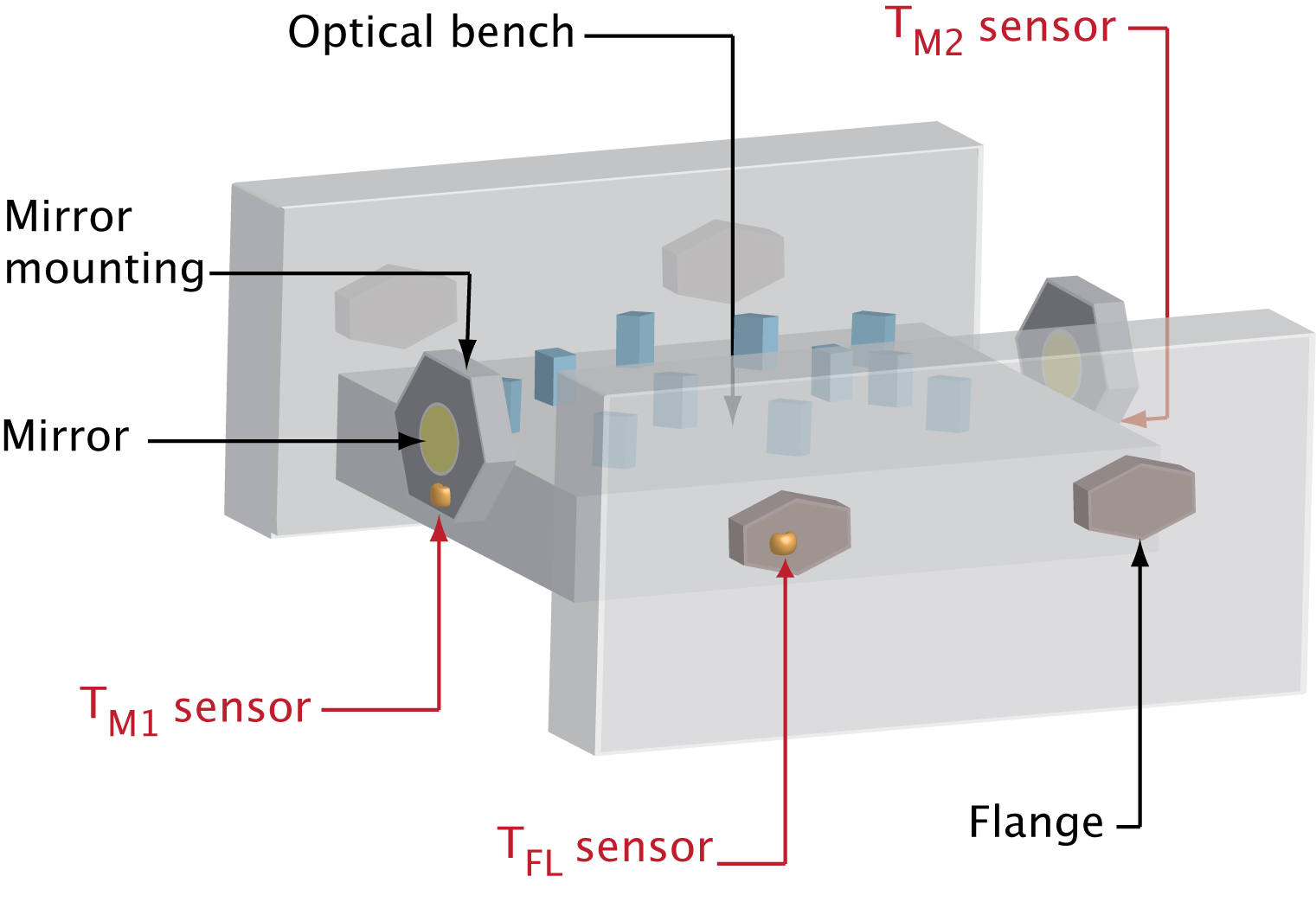
Figure 1: Schematic representation (not to scale) of the location of the temperature sensors in the LISA Pathfinder optical bench. One sensor was attached to each mounting structure supporting the mirrors, a third sensor was attached to the side slab flange —a metallic structure from which the optical bench will be supported inside the satellite thermal shield— and a fourth (not shown) measured the temperature in the laboratory.

The measurements used in our analysis were taken in the LISA Pathfinder engineering model optical bench Heinzel et al. (2003), a close replica of the final bench to be flown in the LISA Pathfinder satellite. In our setup, test masses are substituted by fixed mirrors so only the interferometric metrology subsystem is tested; none of the required drag-free technology used in the final mission is part of our setup. Although the test-bed has shown the required performance in the LISA Pathfinder frequency band, $\rm 1\,mHz\leq f\leq 1\,Hz$ Heinzel et al. (2005); Audley et al. (2011), our main aim was to determine to what extent our measurements were limited by environmental temperature fluctuations and, also, to evaluate this noise contribution in the LISA band. In order to do that, we measured the temperature in four different locations of our setup, as shown in Fig. 1. We initially tested the method using a long data set ($2~{}\times 10^{5}$ s), where the interferometer was running without active noise suppression control loops. With the temperature coupling characterised and the method verified, we then proceeded to subtract the temperature contribution in a shorter, low noise data segment to characterise the impact of this contribution when the interferometer is performing according to the mission requirements, reaching 1 $\rm pm/\sqrt{Hz}$ at 0.1 Hz.

III Experiment characterisation

$\begin{array}[]{cccccc}&&\rm T_{Lab}&T_{Fl}&T_{M1}&T_{M2}\\ &&&&&\\ &&\hbox{\multirowsetup\includegraphics[width=78.04842pt]{figs/coherence_Tlab_ph}}&\hbox{\multirowsetup\includegraphics[width=78.04842pt]{figs/coherence_Tstr_ph}}&\hbox{\multirowsetup\includegraphics[width=78.04842pt]{figs/coherence_Tm1_ph}}&\hbox{\multirowsetup\includegraphics[width=78.04842pt]{figs/coherence_Tm2_ph}}\\ &&&&&\\ \Phi&&&&&\\ &&&&&\\ &&&&&\\ &&&&&\\ &&&&&\\ &&&\hbox{\multirowsetup\includegraphics[width=73.7146pt]{figs/coherence_Tlab_Tstr}}&\hbox{\multirowsetup\includegraphics[width=73.7146pt]{figs/coherence_Tlab_Tm1}}&\hbox{\multirowsetup\includegraphics[width=73.7146pt]{figs/coherence_Tlab_Tm2}}\\ &&&&&\\ \rm T_{Lab}&&&&&\\ &&&&&\\ &&&&&\\ &&&&&\\ &&&&&\\ &&&&\hbox{\multirowsetup\includegraphics[width=73.7146pt]{figs/coherence_Tstr_Tm1}}&\hbox{\multirowsetup\includegraphics[width=73.7146pt]{figs/coherence_Tstr_Tm2}}\\ &&&&&\\ \rm T_{Fl}&&&&&\\ &&&&&\\ &&&&&\\ &&&&&\\ &&&&&\\ &&&&&\hbox{\multirowsetup\includegraphics[width=73.7146pt]{figs/coherence_Tm1_Tm2}}\\ &&&&&\\ \rm T_{M1}&&&&&\\ &&&&&\\ &&&&&\\ &&&&&\\ &&&&&\\ \end{array}$

Figure 2: Setup characterisation. We show the matrix of coherence functions between the different measurements. In the upper row the coherence between interferometer phase and temperature sensors, the rest of figures provide the coherence functions between the different temperature sensors. Units for the x’s values are in hertz.

III.1 Signal processing definitions

We introduce here the basic notation needed to describe our experiment. In general, we could describe our experimental data as a set of q measured temperature time series, $T_{i}(t),\,i=1\ldots q$, which pass through q systems and combine to produce a single measured interferometer output, $\Phi(t)$. The latter will contain a noise contribution which we describe with the random process $n(t)$. If we further assume that our $q$ systems are linear systems, this can be directly translated into the frequency domain as a system of equations

$$\Phi(\omega)=\sum^{q}_{i=1}H_{i}(\omega)\,T_{i}(\omega)+n(\omega),$$ (1)

where $\Phi(\omega)$, $T_{i}(\omega)$ and $n(\omega)$ are the Fourier transforms of the inputs, output and noise contribution respectively, and $H(\omega)$ is the system transfer function. The transfer function is usually estimated from real data by Bendat and Piersol (1993)

$$H_{T_{i}\Phi}(\omega)=\frac{S_{T_{i}\Phi}(\omega)}{S_{T_{i}T_{i}}(\omega)},$$ (2)

where $S_{T_{i}\Phi}(\omega)$ and $S_{T_{i}T_{i}}(\omega)$ are the cross-power spectral density and the power spectral density, which are defined as the Fourier transform of the correlation functions. A second quantity relevant in our case is the coherence function Bendat and Piersol (1993),

$$\gamma^{2}_{T_{i}\Phi}(\omega)=\frac{|S_{T_{i}\Phi}(\omega)|^{2}}{S_{T_{i}T_{i}}(\omega)S_{\Phi\Phi}(\omega)},$$ (3)

which quantifies the amount of correlation between two data sets in each frequency bin. The coherence function turns out to have a particular relevance in our analysis since it allows us to quantify the error on the estimation of the transfer function. To bound the uncertainty of our transfer function estimates, we compute the error on the transfer function as Bendat and Piersol (1993)

$$\sigma\left[|H_{T_{i}\Phi}|\right]\simeq\sigma\left[\theta(H_{T_{i}\Phi})\right]\simeq\frac{\left[1-\gamma^{2}_{T_{i}\Phi}(\omega)\right]^{1/2}}{|\gamma_{T_{i}\Phi}(\omega)|\,\sqrt{2\,n_{d}}},$$ (4)

where $n_{d}$ is the number of averages used to compute the transfer function estimates. The error on the transfer function already contains the information about the correlation between the temperature and the interferometer in the form of the coherence function $\gamma^{2}_{T_{i}\Phi}(\omega)$. By doing this, we ensure that our error estimate takes into account the correlation between temperature and interferometer phase fluctuations. Notice that the same applies to the correlation between temperatures, where we will be using the coherence $\gamma^{2}_{T_{i}T_{j}}(\omega)$ to evaluate the interdependence between temperature variations at each sensor.

III.2 Data preprocessing and characterisation

Before analysing, the data needed to be resampled onto a common time grid. Both the interferometer data (with a sampling frequency of $\rm f_{s}=32.47\,Hz$), and the temperature data (with $\rm f_{s}=1.3\,Hz$) were down-sampled to $\rm f_{s}=1\,Hz$. The temperature sensor data were interpolated to the new time grid with the new sampling frequency, from 1.3 to 1  Hz. In the interferometer case, the data are first down-sampled by a factor of 10 in order to ease data handling, and then resampled to the common grid.

To determine the interdependence between temperature and interferometer readout, we compute the coherence functions between them $\gamma^{2}_{T_{i}\Phi}$. As shown in the upper row of Fig. 2, the three sensors attached to the bench show a coherence above 80% below $f\simeq 0.3$ mHz. As expected, the sensor measuring temperature variations in the lab has the lowest coherence with the interferometer, although still a coherence of 80% can be assigned between interferometer and temperature variations in the lab environment. While at higher frequencies environmental temperature fluctuations can be screened by the vacuum tank; in the low frequency region these fluctuations pass directly through the setup (although delayed, as we show below).

We proceed by determining the interdependence between temperature measured at different locations. In this case, the coherence function is $\gamma^{2}_{T_{i}T_{j}}(\omega)|_{i\neq j}$. Results in Fig. 2 show that the four temperatures are strongly correlated ($\gamma^{2}_{T_{i}T_{j}}(\omega)\simeq 1$), in the very low frequency frequency band ($f<\rm 0.5\,mHz$), and the correlation drops off rapidly above these frequencies. Hence, at the low frequencies of interest, the four measurements contain mostly the same information regarding coupling between interferometer phase and temperature.

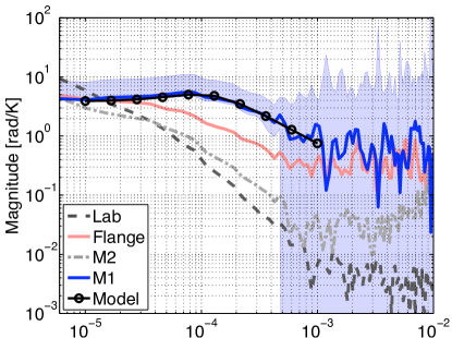
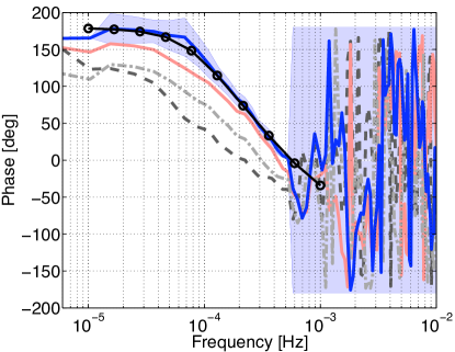
Figure 3: Temperature to interferometer transfer functions for the four sensors in the setup: Lab environment (Lab), optical bench flange (Flange), test mass 2 mirror (M2) and test mass 1 mirror (M1) —see Fig.1 for more details. Errors and fitted model are only shown for the transfer function that shows the highest contribution, i.e. the one coming from the sensor in the first mirror (M1).

Even though the four measurements provide similar temperature information at low frequencies, they do not contribute with the same strength to the interferometric measurement. To show that, we use the transfer function between the temperature data and interferometer data —Eq. (2). In Fig. 3 we show these transfer functions for each sensor; the sensor attached to the first test mass (M1) shows a higher contribution with respect to the other —numerical values for the transfer function are shown in Tab. 1. Also, we computed the group delay of the filter by estimating the slope of the phase of the transfer function for the M1 sensor in the frequency range $\rm 30\,\mu Hz<f<0.2\,mHz$. In our setup, the response of the interferometer to temperature fluctuations below the millihertz frequency band is delayed by $1750\pm 80$ s with respect to the actual time of temperature measurement.

We note that, in our analysis, and as shown in Tab. 1, this correlation is valid for $\rm f\leq 0.5\,mHz$. Therefore, the frequency region where we would expect a noise reduction after subtraction of this contribution would be below the LISA Pathfinder measuring band, but directly affecting a LISA-like measurement.

Table 1: Numerical values for the transfer function corresponding to the sensor in the first mirror mount (M1) and associated errors. Last column shows the coherence function.

Frequency [Hz]	$|\hat{H}_{\varphi T}|$ [rad/K]	$\hat{\gamma}_{\varphi T}$
$1.6\times 10^{-5}$	$4.5\pm 0.5$	0.97
$5.1\times 10^{-5}$	$5.1\pm 0.6$	0.96
$1.1\times 10^{-4}$	$4.5\pm 0.6$	0.91
$2.6\times 10^{-4}$	$2.7\pm 0.5$	0.85
$5.3\times 10^{-4}$	$1.6\pm 2.8$	0.12
$1.0\times 10^{-3}$	$1.4\pm 2.6$	0.10
$2.5\times 10^{-3}$	$0.5\pm 6.5$	0.01

IV Spectral analysis

Once we have characterised our system, our next step is to disentangle the temperature contribution from the interferometer measurement. We will proceed in two different ways: firstly, by solving the linear system and obtaining a set of optimal transfer functions and secondly, by applying a conditioned scheme, which proceeds by solving the linear system for each individual contribution. We describe both in the following section.

IV.1 Optimal spectral analysis

In order to obtain the system of linear equations that will describe our problem we start with Eq. (1),

$$\Phi(\omega)=\sum^{q}_{i=1}H_{i}(\omega)\,T_{i}(\omega)+n(\omega),$$ (5)

where, if we multiply $\Phi(\omega)$ by its complex conjugate $\Phi(\omega)^{*}$, and taking expectation values we obtain

$$S_{nn}=S_{\Phi\Phi}-\sum_{i=1}^{q}H_{i}\,S_{\Phi T_{i}}-\sum_{j=1}^{q}H^{*}_{j}\,S_{T_{j}\Phi}+\sum_{i=j}^{q}\sum_{j=1}^{q}H^{*}_{j}\,H_{i}\,S_{T_{j}T_{i}}.$$ (6)

The optimal solution for this system of equations which minimise $S_{nn}$ over all possible choices of $H_{i}$ is found by setting

$$\frac{\partial S_{nn}}{\partial H_{j}}=0,\quad\frac{\partial S_{nn}}{\partial H^{*}_{j}}=0,$$ (7)

which leads to Bendat and Piersol (1993)

$$S_{T_{j}\Phi}=\sum_{i=1}^{q}H_{i}\,S_{T_{j}T_{i}},\quad j=1,2,\ldots q,$$ (8)

which can be solved for $H_{i}$, since $S_{\Phi T_{i}}$ and $S_{T_{i}T_{j}}$ are known. In our particular case this turns into a system of q = 4 equations, which leads to analytical solutions for $H_{i},\;i=1,\ldots q$. Deriving the expressions for $H_{i}$, which we do not reproduce here, requires us to compute 24 terms for each transfer function, each term containing a product of 4 spectral densities. In the following section we introduce a sequential method which allows us to handle simpler equations, leading to equivalent results.

IV.2 Conditioned spectral analysis

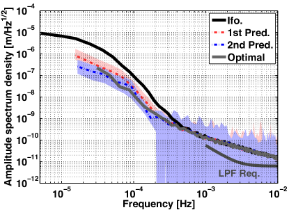
Figure 4: Comparison between optimal and conditioned analysis. The dashed lines (labelled as 1st Pred. and 2nd Pred.) show the expected noise level after subtraction of the two sensors with higher contribution, according to the conditioned analysis scheme. The solid grey (Optimal) line is the expected noise level after an optimal subtraction of all sensors. We show in the same figure the LISA Pathfinder requirement as a reference.

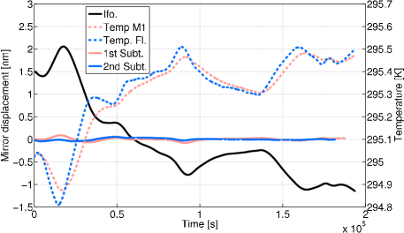
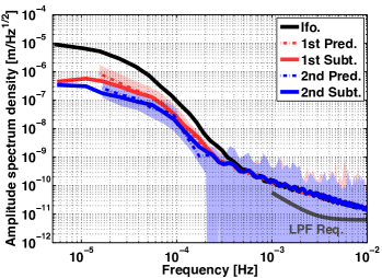
Figure 5: Temperature noise subtraction for a two days measurement without control loops suppressing the interferometric noise contributions. Left: Time domain data series for the two most relevant temperature sensors and the interferometer read out. We also show interferometer data after subtracting the information contained in the two previous temperatures sensors. Right: Comparison of the frequency domain analysis —previously compared with the optimal prediction in Fig. 4— with the spectra of the interferometer time series after the subtraction of the temperature contribution coming from the two most relevant temperature sensors. For comparison, we also show the requirement on interferometric noise in the LISA Pathfinder mission.

A second possible approach is to subtract (in a linear least square sense) one by one those contributions perturbing our measurement. This scheme leads to simpler expressions, which will allow the derivation of the digital filters required to clean the data in the time domain. This approach, known as conditioned spectral analysis, derives the dependence between one of the inputs and the output when the other inputs are turned off, implicitly requiring here that the correlations between inputs are turned off as well. In order to introduce this analysis scheme, we refer back to Eq. (1) which we can write now as

$$\Phi(\omega)=\sum^{q}_{i=1}L_{T_{i}\,\Phi}(\omega)\,T_{i\cdot(i-1)!}(\omega)+n(\omega),$$ (9)

where $T_{i\cdot(i-1)!}(\omega)$ represents the Fourier transform of variable $T_{i}(t)$ when the linear effects of $T_{1}$ to $T_{i-1}$ have been sequentially removed from $T_{i}$ by optimum linear least-squares techniques. Notice that each of this ordered conditioned records will be mutually uncorrelated, a property which is not generally satisfied by the original records. The frequency response function $L_{T_{i}\Phi}$ is the optimum linear system to predict $\Phi(t)$ from $T_{i}(t)$. Analogously as we did in Eq.(6), we can derive the optimum operator, defined as the one that minimises $S_{nn}$ for any possible combination of $L_{T_{i}\Phi}$. This leads to Bendat and Piersol (1993)

$$L_{T_{i}\,\Phi}=\frac{S_{T_{i}\Phi\cdot T_{(i-1)!}}}{S_{T_{i}T_{i}\cdot T_{(i-1)!}}}$$ (10)

where the spectra and cross-spectra appearing in the previous expressions are computed on the conditioned variables. Notice that for the case of a system where q = 1, Eq. (10) and Eq. (8) will naturally reduce to the same expression

$$L_{T_{1}\,\Phi}=H_{1}=\frac{S_{T_{1}\Phi}}{S_{T_{1}T_{1}}}$$ (11)

Following Eq. (3) we can define the coherence function for conditioned variables as

$$\gamma^{2}_{T_{i}\Phi\cdot T_{(i-1)!}}=\frac{|S_{T_{i}\Phi\cdot T_{(i-1)!}}|^{2}}{S_{T_{i}T_{i}\cdot T_{(i-1)!}}S_{\Phi\Phi\cdot T_{(i-1)!}}}$$ (12)

i.e., the coherence between $\Phi$ and $T_{i}$, once all contribution from the previous $i-1$ sensors, $T_{(i-1)!}$, are subtracted. Together with Eq. 10, it can be shown that the conditioned spectra can be written down in terms of partial coherence functions as follows Bendat and Piersol (1993)

$$S_{\Phi\Phi\cdot T_{i!}}=S_{\Phi\Phi\cdot T_{(i-1)!}}\,\left(1-\gamma^{2}_{T_{i}\Phi\cdot T_{(i-1)!}}\right),$$ (13)

where $i=1,2,\ldots q$. This quantity corresponds to the phase noise spectrum, $S_{\Phi\Phi}(\omega)$, when contributions from temperature sensors, $T_{i}$ are recursively removed by linear least squares.

We will use Eq. (13) in the following to obtain predictions of the expected noise reduction when we subtract a given temperature contribution from the main interferometer measurement. This will give us a useful diagnostic tool to evaluate the contribution coming from each location independently. Also, it is worth stressing that, in comparison with the optimal method, the sequential approach in the conditioned scheme allows us to deal with expressions with a maximum of $q$ terms, instead of the $q^{2}$ linear system required in the optimal approach, being $q$ the number of noise contributions in our problem.

V Temperature noise subtraction

V.1 Frequency domain analysis

Before removing the contribution arising from temperature, we proceed to estimate the expected reduction. To do this, we compute the conditioned spectra. Results are shown in Fig. 4 where the curve labelled as ‘prediction’ shows the conditioned spectrum in Eq. (13) for the two sensors with the strongest contributions —according to Fig. 3. We also performed the analysis for a third sensor but the coherence with the interferometer was already too small to show any improvement. In Fig. 4 we also compare the conditioned spectra for the two first subtractions with the spectrum obtained following the optimal subtraction scheme, presented in Sec. IV.1. The comparison confirms that the second subtraction in the conditioned scheme achieves the optimal level and, therefore, subsequent subtractions will not improve substantially. As expected, a coherent subtraction of the temperature contribution would reduce the noise level at frequencies $\rm f\leq 0.4\,mHz$. According to this first analysis, the subtraction of the contribution contained in these two sensors would reduce the instrument noise floor by a factor 5.6 (15 dB) at the very low end of the LISA measurement band, $\rm f=0.1\,mHz$. The factor increases up to 20.2 (26 dB) at the lowest frequency bin, $\rm f=15\,\mu Hz$.

V.2 Time domain analysis

We want to be able to subtract noise contributions in time domain, which can be useful to avoid effects purely related to the Fourier domain, e.g. correlation between frequency bins. Time domain analysis is of relevance as well in order to obtain temperature noise cleaned time-series which can be used for subsequent analysis. For these reasons we have previously resampled both data streams with the same sampling frequency and on to a synchronous time grid. As previously shown, the relation between temperature and phase read out is better described by their frequency domain description. We then translate this transfer function into a digital filter, i.e., a recursive relation that allows us to include a certain dynamical response and, in particular, a delayed action of the temperature upon the interferometer. The tool used here is the vector fitting algorithm Gustavsen and Semlyen (1999) which allows us to fit the measured transfer function in terms of N poles, $p_{k}$, and residues , $z_{k}$,

$$h_{\Phi T_{i}}(z^{-1})=\sum_{k=1}^{N}\frac{r_{k}}{1-p_{k}\,z^{-1}}.$$ (14)

Since our previous analysis showed that the temperature contribution to the interferometer is relevant in a frequency range up to $\rm\simeq 1\,mHz$, we fit the transfer function up to this frequency. Figure 3 shows the fit result with a 3rd order model. Once the digital filter is obtained, we filter the temperature measurement with $h_{\Phi T_{i}}(z^{-1})$ to obtain the temperature contribution to the interferometer, which we can then readily subtract from the original measurement. This procedure is performed initially considering the temperature reading of the sensor attached to the mounting of the first mirror ($\rm T_{\rm M1}$). Then, the information contained in the flange sensor ($\rm T_{\rm FL}$) is removed from the residual of the first subtraction.

As shown in Fig. 5, the subtracted curve is in agreement with the one previously obtained in the frequency domain analysis. We show, for comparison, the LISA Pathfinder interferometric noise goal on the same plot. Since the control loops were not suppressing the interferometric noise contributions, the measurement is above the goal. To further investigate the temperature noise contribution in our setup we used the method above to subtract the temperature noise contribution in a measurement where the instrument was operating in closed-loop (all noise suppression on). The transfer function is the same as the one previously evaluated since the setup remains unchanged. As shown in Fig. 6, the effect of the subtraction reduces the noise level at lower frequencies, $\rm f\leq 0.2\,mHz$, when compared with the control-free case although the effect is stronger at $\rm f=0.1\,mHz$, reducing the noise floor a factor 10 (20 dB) after the subtraction. We notice as well that, according to our current analysis, we can not attribute the complete noise contribution in the low end of the LISA Pathfinder measuring band, $\rm f\simeq 1\,mHz$, to temperature driven phase fluctuations.

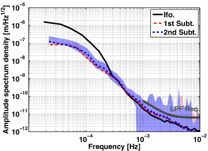
Figure 6: Temperature noise substraction for a data segment where control loops were active. As in previous analysis, we show the subtraction for the two more relevant sensors and we compare with the LISA Pathfinder interferometer noise requirement, showing compliance in this run.

VI Discussion and Conclusions

The analysis reported here characterises, for the first time, the low frequency temperature coupling to an interferometric measurement in a realistic gravitational wave instrumental setup. We also introduce a methodology to clean the main measurement of this noise contribution by removing the information contained in multiple sensors monitoring the experiment. Once applied, we obtain a noise-free time series whose spectral density confirms the prediction obtained by a frequency domain noise projection. We have shown as well that the proposed method, based on conditioned data streams, agrees with the prediction obtained with an optimal approach. The advantage of the former method being a simplification in the required analysis as well as a straightforward characterization of the contribution of each temperature sensor independently. Results on the LISA Pathfinder optical bench show that, when considering the temperature readings in our current setup, the instrument performance is not affected in the Pathfinder measurement band after the temperature noise subtraction, although it gives a significant noise reduction at lower frequencies, and therefore this noise source has a direct impact for LISA-like experiments. This is of relevance for any ground-based gravitational wave experiments aiming at low frequencies, and in particular for those testing technologies for space-based gravitational wave observatories. It is worth stressing that, after temperature noise subtraction, our experiment shows a performance of $100\,\rm nm/\sqrt{Hz}$ at f = 30 $\rm\mu Hz$. This precision at very low frequencies in an optical metrology measurement can only be compared with results from a recent test campaign of the LISA Pathfinder spacecraft in an artificial space environment Cervantes et al. (2013), which further confirms that the method described here can allow on-ground lab experiments to compute a performance curve without the limitation of the unavoidable temperature drifts, achieving results which are close to space conditions. The method is extendable as well to any frequency dependent contribution that is independently measurable in gravitational wave experiments.