Bifurcations and exceptional points in dipolar Bose-Einstein condensates

Abstract

Bose-Einstein condensates are described in a mean-field approach by the nonlinear Gross-Pitaevskii equation and exhibit phenomena of nonlinear dynamics. The eigenstates can undergo bifurcations in such a way that two or more eigenvalues and the corresponding wave functions coalesce at critical values of external parameters. E.g. in condensates without long-range interactions a stable and an unstable state are created in a tangent bifurcation when the scattering length of the contact interaction is varied. At the critical point the coalescing states show the properties of an exceptional point. In dipolar condensates fingerprints of a pitchfork bifurcation have been discovered by Rau et al[Phys. Rev. A, 81:031605(R), 2010]. We present a method to uncover all states participating in a pitchfork bifurcation, and investigate in detail the signatures of exceptional points related to bifurcations in dipolar condensates. For the perturbation by two parameters, viz. the scattering length and a parameter breaking the cylindrical symmetry of the harmonic trap, two cases leading to different characteristic eigenvalue and eigenvector patterns under cyclic variations of the parameters need to be distinguished. The observed structures resemble those of three coalescing eigenfunctions obtained by Demange and Graefe [J. Phys. A, 45:025303, 2012] using perturbation theory for non-Hermitian operators in a linear model. Furthermore, the splitting of the exceptional point under symmetry breaking in either two or three branching singularities is examined. Characteristic features are observed when one, two, or three exceptional points are encircled simultaneously.

1 Introduction

The macroscopic occupation of the bosonic ground state of ultracold quantum gases has been predicted by Bose and Einstein, and at least since the first realisation of Bose-Einstein condensates (BECs) [1, 2, 3] they are a central part of experimental and theoretical atomic physics. The condensates are typically held in a harmonic trap. The particles in the trap interact via short-range contact interactions determined by the s-wave scattering length $a$, which can be varied experimentally with the help of Feshbach resonances. In addition long-range interactions exist, e.g., in dipolar condensates [4] or in condensates with an attractive $1/r$ interaction [5, 6].

In a mean-field approach the effective one-particle wave function of the condensate is described by the nonlinear Gross-Pitaevskii equation (GPE). The nonlinearity of the GPE allows for a variety of phenomena which are impossible in linear quantum systems with Hermitian operators. For example, the extended Gross-Pitaevskii equation for a BEC without long-range interactions or with an attractive $1/r$ interaction has a second solution which emerges together with the ground state in a tangent bifurcation [6]. At the bifurcation point both states coalesce, i.e., the energies and the wave functions are identical. It has been shown [7] that the bifurcation point has the properties of an “exceptional point” [8, 9, 10, 11, 12]. Such points can appear in systems described by non-Hermitian matrices which depend on a two-dimensional parameter space. The exceptional points are critical points in the parameter space where both the eigenvalues and the eigenvectors of the two states pass through a branch point singularity and become identical. There is only one linearly independent eigenvector of the two states at an exceptional point.

Bifurcation scenarios become even more substantial in dipolar condensates. With a simple variational approach a tangent bifurcation between the ground state and an unstable excited state was observed in [13], and it was shown that the bifurcation point has the properties of an exceptional point. However, using an extended variational approach with coupled Gaussians for the condensate wave function the ground state is created unstable and only becomes stable at an increased value of the scattering length [14]. Although no bifurcating states have been directly computed in [14], the stability change indicates the existence of a pitchfork bifurcation, which means that three states coalesce at the bifurcation point.

The detailed investigation of pitchfork bifurcations and signatures of three coalescing eigenfunctions in dipolar condensates is the objective of this paper. We present a method which exploits the symmetry breaking of the external harmonic trap and allows us to reveal all three states involved in the pitchfork bifurcation. The energies and the eigenfunctions of the three states coalesce at the bifurcation point, however, the degeneracies are lifted when the scattering length is varied or the axial symmetry of the harmonic trap is broken.

The signatures of three coalescing eigenfunctions have been investigated by Demange and Graefe [15] using perturbation theory for a model with linear but non-Hermitian operators. It was shown that two types of parameter perturbations need to be distinguished, which are related to a cubic root and a square root branching singularity at the exceptional point and lead to characteristic patterns under cyclic variation of the parameters. With an analytic continuation of the nonlinear GPE in the two parameters, viz. the scattering length and a parameter breaking the axial symmetry of the harmonic trap, we show that the signatures of the three states of a dipolar BEC which coalesce in the pitchfork bifurcation exactly resemble those obtained in the linear model [15] with complex non-Hermitian matrices. Both, the cubic root and the square root branching singularity are observed when encircling the exceptional point either in the symmetry breaking parameter or in the scattering length. Furthermore, we will discuss the behaviour of the eigenvalues and eigenvectors when both control parameters are simultaneously varied.

2 Variational approach to dipolar condensates

An extended variational ansatz with coupled Gaussian functions has been used by Rau et al[16, 17] to compute numerically accurate solutions of the GPE for condensates with dipolar interactions. Contrary to the numerical imaginary time evolution of states on grids the variational approach allows for the calculation of not only the ground state but also excited states, which is a prerequisite for the investigation of bifurcation scenarios and exceptional points. In this section we briefly recapitulate the variational method and introduce the analytic continuation of the GPE, which then allows for the encircling of exceptional points in the complex parameter space.

We use the time-dependent GPE in dimensionless and particle number scaled units (see [13]),

$$H\psi(\bm{r},t)=[-\Delta+V]\psi(\bm{r},t)=\rmi\frac{\partial}{\partial t}\psi(\bm{r},t)\;,$$ (1)

to describe dipolar BECs in the mean-field approximation. The total potential

$$V=V_{\rm t}+V_{\rm c}+V_{\rm d}$$ (2)

is composed of three parts. The external trap is described by the harmonic potential

$$V_{\rm t}=\gamma_{x}^{2}x^{2}+\gamma_{y}^{2}y^{2}+\gamma_{z}^{2}z^{2}\;,$$ (3)

where the $\gamma_{x,y,z}$ determine the strength of the trap in the $x$, $y$, and $z$ directions. The dipolar condensates are typically held in an axisymmetric trap with $\gamma_{x}=\gamma_{y}$. In order to describe the trap frequencies in a way that represents the trap geometry and to allow us to change the trap symmetry by modifying only one parameter we will use the parametrisation

$$\gamma_{x}=\bar{\gamma}(1+s)^{1/2}\lambda^{-1/3}\;,\quad\gamma_{y}=\bar{\gamma}(1+s)^{-1/2}\lambda^{-1/3}\;,\quad\gamma_{z}=\bar{\gamma}\lambda^{2/3}$$ (4)

where $\bar{\gamma}$ is the average trap frequency and $\lambda$ the ratio between the trap frequency in $z$-direction and the trap frequencies in the $x,y$-plane. The asymmetry parameter $s$ breaks, for $s\neq 0$, the axial symmetry of the trap, and is one of the two parameters used below to examine the signatures of exceptional points. The potential

$$V_{\rm c}=8\pi a|\psi(\bm{r},t)|^{2}$$ (5)

describes the short-range contact interactions resulting from s-wave scattering between particles with $a$ the (scaled) scattering length. The scattering length $a$ is the second parameter used to examine the signatures of exceptional points. Finally, the potential

$$V_{\rm d}=\int\rmd^{3}r^{\prime}\frac{1-3\cos^{2}\vartheta}{|\bm{r}-\bm{r^{\prime}}|^{3}}|\psi(\bm{r}^{\prime},t)|^{2}$$ (6)

describes the dipole-dipole interaction between particles with a magnetic moment, with $\vartheta$ the angle between the vector $\bm{r}-\bm{r}^{\prime}$ and the $z$-axis along which all dipoles are aligned by an external magnetic field.

In order to solve the GPE (1) we use the time-dependent variational principle (TDVP) [18]. The idea of the TDVP is to use an ansatz for the wave function depending on the set of variational parameters $\bm{z}$ and then choose these parameters in such a way that the quantity $I=\|H\psi-\rmi\dot{\psi}\|^{2}$ is minimised. We use a superposition of $N$ Gaussian functions

$$\psi(\bm{r},\bm{z})=\sum_{k=1}^{N}g^{k}=\sum_{k=1}^{N}\rme^{-\left(A_{x}^{k}x^{2}+A_{y}^{k}y^{2}+A_{z}^{k}z^{2}+\gamma^{k}\right)}$$ (7)

as an ansatz for the wave function, where the $A_{\sigma}^{k}$ are the complex width parameters of the $k$th Gaussian in $\sigma$ direction, and the real and imaginary parts of the $\gamma^{k}$ describe the phase and the amplitude of the $k$th Gaussian, respectively. The variational parameters are combined in the complex vector

$$\bm{z}=\left(\gamma^{1},\dots,\gamma^{N},A_{x}^{1},\dots,A_{x}^{N},A_{y}^{1},\dots,A_{y}^{N},A_{z}^{1},\dots,A_{z}^{N}\right)\in\mathbb{C}^{4N}\;.$$ (8)

The application of the TDVP (for details of the derivations see [16]) leads to the following equations of motion. The time derivatives of the variational parameters are given by $\dot{\bm{z}}=\bm{h}(\bm{z})$, or in components

$$\dot{\gamma}^{k} =2\rmi\left(A_{x}^{k}+A_{y}^{k}+A_{z}^{k}\right)+\rmi v_{0}^{k}\;,$$

$$\dot{A}_{\sigma}^{k} =-4\rmi(A_{\sigma}^{k})^{2}+\rmi v_{\sigma}^{k}\quad{\rm with}\quad\sigma=x,y,z\;.$$ (9)

The quantities $v_{0}^{k}$ and $v_{\sigma}^{k}$ in equation (9) can be written as a vector $\bm{v}=(v_{0}^{1},\dots,v_{0}^{N},v_{x}^{1},\dots,v_{x}^{N},v_{y}^{1},\dots,v_{y}^{N},v_{z}^{1},\dots,v_{z}^{N})$, which is obtained by solving the linear system of equations

$$M\bm{v}=\bm{r}\;.$$ (10)

The matrix $M$ has the form

$$M=\left(\begin{array}[]{cccc}\left(1\right)_{lk}&\left(x^{2}\right)_{lk}&\left(y^{2}\right)_{lk}&\left(z^{2}\right)_{lk}\\ \left(x^{2}\right)_{kl}&\left(x^{4}\right)_{lk}&\left(x^{2}y^{2}\right)_{lk}&\left(x^{2}z^{2}\right)_{lk}\\ \left(y^{2}\right)_{kl}&\left(x^{2}y^{2}\right)_{kl}&\left(y^{4}\right)_{lk}&\left(y^{2}z^{2}\right)_{lk}\\ \left(z^{2}\right)_{kl}&\left(x^{2}z^{2}\right)_{kl}&\left(y^{2}z^{2}\right)_{kl}&\left(z^{4}\right)_{lk}\end{array}\right)$$ (11)

with the submatrices

$$(O)_{lk}=\langle g^{l}|O|g^{k}\rangle$$ (12)

for $k,l=1,\dots,N$ and the operators $O=1,x^{2},y^{2},z^{2},x^{2}y^{2},x^{2}z^{2},y^{2}z^{2},x^{4},y^{4},z^{4}$. The components of the right-hand side vector $\bm{r}=(r_{1}^{1},\dots,r_{1}^{N},r_{x}^{1},\dots,r_{x}^{N},r_{y}^{1},\dots,r_{y}^{N},r_{z}^{1},\dots,r_{z}^{N})$ in equation (10) read

$$r_{f}^{l}=\sum_{k=1}^{N}\langle g^{l}|f^{2}\,V|g^{k}\rangle$$ (13)

for $f=1,x,y,z$ and $l=1,\dots,N$. All components of the matrix $M$ and the integrals for the vector $\bm{r}$ in equation (13) are listed in A. The components of the matrix $M$ can be expressed analytically. The vector $\bm{r}$ is more complicated due to the dipole interaction. The components

$$\langle g^{k}|f^{2}\,V_{\rm d}|g^{l}\rangle\leavevmode\nobreak\ \leavevmode\nobreak\ {\rm with}\leavevmode\nobreak\ f=1,x,y,z$$ (14)

lead to expressions which contain elliptic integrals of the form

$$R_{D}(x,y,z)=\frac{3}{2}\int_{0}^{\infty}\frac{\rmd t}{\sqrt{(x+t)(y+t)(z+t)^{3}}}\;.$$ (15)

These integrals can be calculated numerically using the Carlson algorithm [19].

The stationary states are obtained as fixed points of the equations of motion (9), i.e. $\dot{\gamma}^{k}-\rmi\mu=0$ and $\dot{A}_{\sigma}^{k}=0$ with $\mu$ the chemical potential, $\sigma=x,y,z$, and $k=1,\dots,N$. The set of the variational parameters $\gamma$ can be reduced to $\tilde{\gamma}^{k}=\gamma^{k}-\gamma^{1}$ for $k=2,\dots,N$ by using the facts that the wave function is normalised to $\langle\psi|\psi\rangle=1$ and a global phase of the wave function is arbitrary. The conditions for a stationary state then simplify to

$$\dot{\tilde{\gamma}}^{k} = \dot{\gamma}^{k}-\dot{\gamma}^{1}=0\;;\quad k=2,\dots,N\;,$$

$$\dot{A}_{x}^{k} = \dot{A}_{y}^{k}=\dot{A}_{z}^{k}=0\;;\quad k=1,\dots,N\;.$$ (16)

The root search for the fixed points is performed using the Newton-Raphson algorithm.

The mean-field energy of a stationary state is given by

$$E_{\rm mf}=\langle\psi|-\Delta+V_{\rm t}+\textstyle{\frac{1}{2}}(V_{\rm c}+V_{\rm d})|\psi\rangle\;,$$ (17)

and can be used to examine some properties of the state. However, the typical bifurcation behaviour is revealed even more clearly by, e.g. the expectation values $w$ of the operator $x^{2}-y^{2}$, viz.

$$w=\langle\psi|x^{2}-y^{2}|\psi\rangle\;,$$ (18)

and therefore this value is used below in most cases to reveal the bifurcations and to analyse the signatures of the exceptional points. For the presentation of the splittings we use the distance from their mean values,

$$\Delta E_{{\rm mf},j} = E_{{\rm mf},j}-\frac{1}{N_{\rm s}}\sum_{i=1}^{N_{\rm s}}E_{{\rm mf},i}\;,$$ (19)

$$\Delta w_{j} = w_{j}-\frac{1}{N_{\rm s}}\sum_{i=1}^{N_{\rm s}}w_{i}\;,$$ (20)

i.e. the mean values of the quantities of all $N_{\rm s}$ states participating in the bifurcation (with $N_{\rm s}=2$ for a tangent bifurcation and $N_{\rm s}=3$ for a pitchfork bifurcation) are subtracted. The index $j$ indicates the $j$th state $|\psi_{j}\rangle$ of the bifurcation. With the new values the level-splittings at the bifurcations (which are small compared to the absolute values) can be clearly observed.

The linear stability of stationary states is analysed by calculating the eigenvalues of the Jacobi matrix

$$J_{ij}=\frac{\partial\dot{\tilde{z}}_{i}}{\partial\tilde{z}_{j}}\;,$$ (21)

which is obtained with the variational parameters split into their real and imaginary parts, viz.

$$\tilde{\bm{z}}=({\rm Re}\,z_{1},{\rm Im}\,z_{1},\dots,{\rm Re}\,z_{4N},{\rm Im}\,z_{4N})\in\mathbb{R}^{8N}\;.$$ (22)

If all eigenvalues are purely imaginary, the state is stable, otherwise it is unstable. The eigenvalues occur in pairs $\pm\lambda$. If one pair of eigenvalues has a nonzero real part the state is unstable in the directions of the associated eigenvectors in the parameter space. If two pairs of eigenvalues have a nonzero real component the state is unstable in four directions, and so on.

2.1 Analytic continuation of the GPE

The parameter $s$ in equation (4), which breaks the axial symmetry of the harmonic trap, and the scattering length $a$ in equation (5) are the two, physically real, parameters used to control the system. To investigate a bifurcation point in equation (9) for the signatures of an exceptional point it is necessary to encircle the critical value in the complex plane. Therefore, the GPE (1) must be continued analytically with respect to the parameters $s$ and $a$ in such a way that observables, such as the mean-field energy $E_{\rm mf}$ or the value of $w$, can become complex. As the variational parameters $\bm{z}\in\mathbb{C}^{4N}$ are complex parameters it is necessary to split the components into their real and imaginary parts, and to start with the real parameters $\tilde{\bm{z}}\in\mathbb{R}^{8N}$ introduced in equation (22). The real components of the vector $\tilde{\bm{z}}$ can now be continued analytically as

$$\tilde{z}_{l}=\tilde{z}_{l}^{R}+{\rm k}\tilde{z}_{l}^{I}$$ (23)

with the real parameters $z_{l}^{R}$ and $\tilde{z}_{l}^{I}$ for $l=1,\dots,8N$, and the imaginary unit ${\rm k}$ defined by ${\rm k}^{2}=-1$. It is important to distinguish ${\rm k}$ from the imaginary unit $\rmi$ for the following reason. The complex conjugate of the wave function $\psi(\bm{r},\bm{z})$ in equation (7) is obtained by the replacement $\rmi\to-\rmi$ and thus $\bm{z}\to\bm{z}^{\ast}$, however, the sign of ${\rm k}$ in the complex continued vector $\tilde{z}$ in equation (23) must not be changed. Formally, the variational parameters $\bm{z}$ can be written as bicomplex numbers

$$z_{l} =z_{l}^{R}+\rmi\,z_{l}^{I}=(z_{l,1}+{\rm k}\,z_{l,2})+\rmi\,(z_{l,3}+{\rm k}\,z_{l,4})$$ (24)

$$=z_{l,1}+{\rm k}\,z_{l,2}+\rmi\,z_{l,3}-{\rm j}\,z_{l,4}$$

with $\rmi^{2}={\rm k}^{2}=-1$, ${\rm j}^{2}=1$, $\rmi{\rm j}={\rm j}\rmi={\rm k}$, ${\rm j}{\rm k}={\rm k}{\rm j}=\rmi$, and $\rmi{\rm k}={\rm k}\rmi=-{\rm j}$. The complex conjugate wave function in this description has the form

$$\psi^{\ast}(\bm{r})=\sum_{l=1}^{N}\rme^{-\left(A_{x}^{l\ast}x^{2}+A_{y}^{l\ast}y^{2}+A_{z}^{l\ast}z^{2}+\gamma^{l\ast}\right)}\;,$$ (25)

with $A_{\sigma}^{l\ast}=(A_{\sigma,1}^{l}+{\rm k}A_{\sigma,2}^{l})-\rmi(A_{\sigma,3}^{l}+{\rm k}A_{\sigma,4}^{l})$ and $\gamma^{l\ast}=(\gamma_{1}^{l}+{\rm k}\gamma_{2}^{l})-\rmi(\gamma_{3}^{l}+{\rm k}\gamma_{4}^{l})$. For complex parameters $s$ and $a$ the analytically continued equations of motion (9) can now be set up for the variational parameters extended to bicomplex numbers. The advantage of using bicomplex numbers is that the rules for calculations can be easily implemented in computer algorithms, e.g. by introducing a new data type and overloading operators. In particular, Carlson’s algorithm [19] for the computation of the elliptic integrals $R_{D}(x,y,z)$ in equation (15) can be used with nearly no modifications for real, complex, and even bicomplex numbers $x$, $y$, and $z$. The linear set of equations (10) can be solved either directly with bicomplex numbers or the components of the bicomplex matrix $M$, and the vectors $\bm{v}$ and $\bm{r}$ can be split into two complex numbers to set up an ordinary complex linear system of equations of twice the dimension.

The stationary states are obtained as roots of equations (16) extended to bicomplex variational parameters. Note that with the analytic continuation observables such as the mean-field energy $E_{\rm mf}$ or the value of $w$ are not necessarily real but can become complex valued, e.g. $w=w_{1}+{\rm k}w_{2}$ with the $\rmi$ and ${\rm j}$ components $w_{3}=w_{4}=0$. In the following we use the notation ${\rm Re}\,w=w_{1}$ and ${\rm Im}\,w=w_{2}$ in such cases.

3 Bifurcations of the stationary states

We study the bifurcation scenarios of the stationary states of a dipolar BEC in a harmonic trap for the case that the average trap frequency $\bar{\gamma}$, the ratio $\lambda$, and the symmetry breaking parameter $s$ in equation (4) are kept constant and the scattering length $a$ is varied.

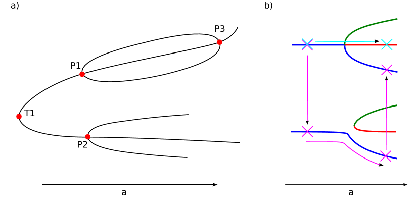
Figure 1: (a) Sketch of the bifurcation scenario of a dipolar BEC in an axisymmetric trap. Two states emerge in a tangent bifurcation at T1. The two branches undergo pitchfork bifurcations at P1 and P2. The three states created in the pitchfork bifurcation P1 merge again in an inverse pitchfork bifurcation at P3. (b) Scheme how to find the branching states of the pitchfork bifurcation: Starting at $s=0$ on the central state marked by a cross in the left-hand upper part of the figure the axial symmetry of the trap is broken (cross in the lower part of the figure), then the state is followed adiabatically by increasing the scattering length, and finally the axial symmetry of the trap is restored to end up with a state on one of the symmetry breaking branches in the upper part of the figure.

A sketch of the bifurcation scenario is given in figure 1(a). The ground state and an excited state emerge in a tangent bifurcation (marked T1 in figure 1(a)) at a critical scattering length $a=a_{\rm T1}$ [13, 17]. When the scattering length is increased both the ground and the excited state can undergo further bifurcations indicated P1, P2, and P3 in figure 1(a).

3.1 Bifurcations of the excited state

We start with the investigation of the stationary states using a single Gaussian function as a variational ansatz for the wave function. The trap parameters are set to $\bar{\gamma}_{1}=34000$, $\lambda_{1}=6$, and $s=0$ for a harmonic potential with axial symmetry, which is in the region where dipolar condensates with chromium atoms have been realised experimentally [20, 4]. The bifurcation scenario drafted in figure 1(a) (without P2) emerges. At the scattering length $a_{\rm T1}=-0.019$ a stable ground state and an unstable excited state are created in a tangent bifurcation (T1). Both wave functions are axisymmetric around the $z$ axis. At the scattering length $a_{\rm P1}=-0.0079$ the excited state undergoes a pitchfork bifurcation P1, where its stability properties change from unstable for one pair of stability eigenvalues to unstable for two pairs of stability eigenvalues. If the scattering length is further increased all three states which emerge in the pitchfork bifurcation are recombined in an inverse pitchfork bifurcation at $a_{\rm P3}=0.129$. At the bifurcation points not only the mean-field energies and the expectation values of the operator $x^{2}-y^{2}$ but also the wave functions coalesce.

In figure 2(a)-(b) the detailed results for the pitchfork bifurcation P1 around the critical scattering length $a_{\rm P1}=-0.0079$ are presented.

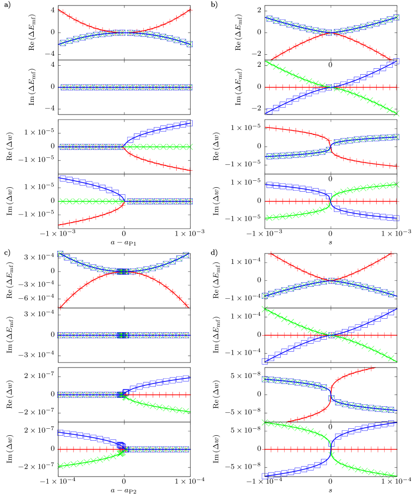
Figure 2: (a)-(b) Level splittings of the mean-field energy $E_{\rm mf}$ and the values $w=\langle\psi|x^{2}-y^{2}|\psi\rangle$ around the pitchfork bifurcation P1 of the excited state. The symbols and solid lines mark the results of the GPE using a variational ansatz with a single Gaussian function and the linear model introduced in section 3.3, respectively. In (a) the scattering length is varied for a symmetric trap ($s=0$) and in (b) the asymmetry parameter $s$ is varied while the scattering length is kept constant ($a=a_{\rm P1}$). (c)-(d) Results for the pitchfork bifurcation P2 of the ground state. Here, the GPE was solved using an ansatz with six coupled Gaussians.

Shown are both the real branches and the complex branches obtained by analytic continuation of the GPE. The characteristic shape of a pitchfork bifurcation is evident in the real part of $\Delta w$ in figure 2(a), where two new real branches emerge at the bifurcation point $a_{\rm P1}=-0.0079$. The new emerging states are unstable with one pair of stability eigenvalues with nonzero real part, and the corresponding wave functions break the axial symmetry of the trap. The two states only differ by a $90^{\circ}$ rotation around the $z$ axis. With the analytic continuation two additional complex branches are found below the bifurcation point as can be seen in the imaginary part of $\Delta w$ in figure 2(a).

The existence of a new branch at $a>a_{\rm P1}$ is also visible in figure 2(a) for the splitting $\Delta E_{\rm mf}$ of the mean-field energy. As the two new states only differ by a $90^{\circ}$ rotation around the $z$ axis in the axisymmetric trap the mean-field energy of the new branch is twofold degenerate. Furthermore, the splitting $\Delta E_{\rm mf}$ increases quadratically with $a-a_{\rm P1}$ in contrast to the typical square root behaviour of a pitchfork bifurcation, and the mean-field energy is real also for those states obtained with the analytic continuation of the GPE in the region $a<a_{\rm P1}$, i.e. ${\rm Im}\,(\Delta E_{\rm mf})=0$ for all states in figure 2(a).

When the scattering length is kept constant at $a=a_{\rm P1}$ and the asymmetry parameter $s$ is varied the splittings $\Delta E_{\rm mf}$ and $\Delta w$ show a quite different cubic-root-like behaviour as illustrated in figure 2(b). The splitting is $\Delta E_{\rm mf}\sim s^{4/3}$ for the mean-field energy and $\Delta w\sim s^{1/3}$ for the expectation values of the operator $x^{2}-y^{2}$, which implies that the splittings are real-valued only for the central state marked by red plus symbols in figure 2(b). A more detailed discussion of the splittings based on a linear model with non-Hermitian matrices will be presented in section 3.3.

3.2 Bifurcations of the ground state

Using the simple variational approach with a single Gaussian function ($N=1$) the stable ground state emerges in a tangent bifurcation [13]. However, the situation becomes more complicated when using an improved and extended ansatz with coupled Gaussians for the condensate wave function [14, 16, 17]. For $N=6$ Gaussian functions and an external trap with parameters $\bar{\gamma}_{2}=6887$, $\lambda_{2}=7$, and $s=0$ the ground state is created unstable in the tangent bifurcation and then becomes stable at a larger value of the scattering length. The stability change exhibits fingerprints of a pitchfork bifurcation, however, the numerical search for the new branches emerging in the bifurcation is a very nontrivial task in the dimensionally increased parameter space for coupled Gaussians and thus have not been computed in [17]. Here we present a method based on breaking the axial symmetry of the harmonic trap to obtain the additional states emerging in the pitchfork bifurcation.

The method consists of three steps as illustrated in figure 1(b). Starting with an axisymmetric state ($s=0$) at a scattering length below the bifurcation point the asymmetry parameter $s$ is varied in a first step to break the axial symmetry of that state ($s\neq 0$). In a second step the scattering length $a$ is increased to a value greater than the critical value of the pitchfork bifurcation. Using small increments of the scattering length we can follow the state adiabatically as shown in figure 1(b). In a third step the parameter $s$ is changed back to $s=0$ for the axisymmetric trap, however, the state at the end of this path belongs to one of the new branches emerging in the pitchfork bifurcation. The other branch can be reached in the same way with the asymmetry parameter $s$ changed in the opposite direction.

The states of the new branches break the axial symmetry around the $z$ axis and differ by a $90^{\circ}$ rotation in a similar way as discussed for the pitchfork bifurcation of the excited state in section 3.1. The resulting branches of the pitchfork bifurcation P2 in the ground state branch can be seen as functions of the scattering length $a-a_{\rm P2}$ and the asymmetry parameter $s$ in figure 2(c) and (d), respectively. Up to a change in sign of the splittings $\Delta E_{\rm mf}$ and $\Delta w$ the results qualitatively agree with those of the bifurcation P1 of the excited state in figure 2(a)-(b). The eigenvalues and eigenvectors of all three states coincide at the critical scattering length $a_{\rm P2}=-0.0036$ of the pitchfork bifurcation.

3.3 Linear model with non-Hermitian matrices

The bifurcations and exceptional points in dipolar condensates result from the nonlinearity of the GPE (1). Nevertheless, we now introduce a linear model with non-Hermitian matrices which can reproduce the pitchfork bifurcations shown in figure 2 and the level splittings of both the mean-field energies $\Delta E_{{\rm mf},j}$ and the values $\Delta w_{j}$ as defined in equations (19) and (20), respectively. Furthermore, the linear matrix model can describe the observed structures when an exceptional point related to one of the pitchfork bifurcations is encircled in either the asymmetry parameter $s$ or the scattering length $a$ as discussed in section 4, and is even valid for the two parameter perturbations discussed in section 4.2.

The values of $\Delta w_{j}$ are obtained as eigenvalues of the non-Hermitian matrix

$$Q_{w}=c_{w}\left(\begin{array}[]{ccc}0&1&0\\ \tilde{a}&0&1\\ s&0&0\end{array}\right)\;,$$ (26)

where $s$ is the asymmetry parameter, and

$$\tilde{a}=c_{a}(a-a_{\rm cr})$$ (27)

is the rescaled and shifted scattering length so that the critical value $a_{\rm cr}$ of the bifurcation is at $\tilde{a}=0$. Equation (20) ensures that the matrix $Q_{w}$ is traceless, and $c_{w}$ and $c_{a}$ are real parameters, which depend on the values $\bar{\gamma}$ and $\lambda$ of the trap potential and are determined by a least-squares fit using the data obtained with the TDVP as described in section 2. For $\tilde{a}=0$ and $s=0$ the matrix $Q_{w}$ has the Jordan form of an EP3 with eigenvalue $\lambda=0$ (see section 4). The solid lines for the real and imaginary part of $\Delta w$ in figure 2 present the eigenvalues of the matrix $Q_{w}$ with $c_{a}=26.180$ and $c_{w}=-1.0780\times 10^{-4}$ for the pitchfork bifurcation P1 and $c_{a}=104.46$ and $c_{w}=1.8436\times 10^{-6}$ for the pitchfork bifurcation P2. For $s=0$ one eigenvalue is zero and two eigenvalues are $\sim\sqrt{a-a_{\rm cr}}$, and for $\tilde{a}=0$ all three eigenvalues are $\sim s^{1/3}$. Obviously, the results of the matrix model perfectly agree with the exact data marked by symbols in figure 2.

The matrix model for the mean-field energy is somewhat more complicated. For the simplicity of the model we require that the matrix elements are low-order power functions of $\tilde{a}$ and $s$, and the eigenvalues are $\sim\tilde{a}^{2}$ for $s=0$ and $\sim s^{4/3}$ for $\tilde{a}=0$. Furthermore, we require that for $s\neq 0$ both matrices $Q_{w}$ and $Q_{E}$ always have the same number of degenerate eigenvalues when the two parameters $\tilde{a}$ and $s$ are varied (see section 4.2 for more details). The matrix

$$Q_{E}=c_{E}\left(\begin{array}[]{ccc}\tilde{a}^{2}&9s&2\tilde{a}\\ 16\tilde{a}s&\tilde{a}^{2}&9s\\ 9s^{2}&0&-2\tilde{a}^{2}\end{array}\right)$$ (28)

fulfils these requirements. The real coefficients $c_{a}$ and $c_{E}$ are determined by least-squares fits, and read $c_{a}=26.182$ and $c_{E}=-3136.3$ for the pitchfork bifurcation P1 and $c_{a}=101.76$ and $c_{E}=4.0582$ for the pitchfork bifurcation P2 in figure 2. The eigenvalues of the matrix $Q_{E}$ shown as solid lines in the graphs for $\Delta E_{\rm mf}$ agree perfectly with the exact data marked by symbols.

4 Exceptional points

The coalescence of two eigenvalues and the corresponding eigenvectors is a feature known as “exceptional point” [8, 9, 10], and such an EP2 can appear in systems described by non-Hermitian matrices, which depend on at least a two-dimensional parameter space. When the exceptional point is encircled in the two-dimensional parameter space the eigenvalues show a characteristic feature of a square root branching singularity, which is that the two eigenvalues permute after one cycle in the parameter space, and the initial configuration of the eigenvalues is obtained only after two cycles in the parameter space. The degeneracy of more than two eigenvalues and eigenvectors is possible, in principle, however, an EP$n$ in general requires the adjustment of $(n^{2}+n-2)/2$ parameters [11], which implies e.g. that $5$ parameters are necessary for an EP3.

The signatures of coalescing eigenfunctions have been studied by Demange and Graefe [15] for complex non-Hermitian matrices. If these matrices are transformed to their Jordan normal form, the type of the exceptional point is given by the size of the Jordan block. For example, a block of size three

$$J_{\rm EP3}=\left(\begin{array}[]{ccc}\lambda&1&0\cr 0&\lambda&1\cr 0&0&\lambda\end{array}\right)$$ (29)

characterises an EP3. Now a perturbation can be added to $J_{\rm EP3}$, viz.

$$J_{\rm EP3}^{\ast}=J_{\rm EP3}+\Omega P\leavevmode\nobreak\ {\rm with}\leavevmode\nobreak\ P\in\mathbb{C}^{3\times 3}\;.$$ (30)

If $\Omega$ describes a complex path which encircles the exceptional point, e.g. $\Omega(\varphi)=\rme^{\rmi\varphi}$, the behaviour of the eigenvalues depends on properties of the perturbation. If the perturbation matrix $P$ is such that the element

$$P_{31}\neq 0\,,$$ (31)

then the typical cubic-root branching singularity expected for an EP3 [11] is observed, i.e. all three eigenvalues and eigenstates permute. However, if the condition (31) is not fulfilled one might observe the permutation between two states, i.e. the signature of a square-root branching singularity [15].

In a dipolar BEC with an axisymmetric trap the eigenvalues and the eigenvectors of three states coincide in a pitchfork bifurcation by varying only a single parameter, viz. the scattering length $a$ of the contact interaction. The coalescence of three states by varying only one parameter is certainly related to an underlying high symmetry of the system. In this section we investigate in detail the signatures of the exceptional points occurring in dipolar condensates.

4.1 Encircling the exceptional points

We examine the permutation behaviour of the stationary states when the bifurcation points are enclosed by a parameter path. Using the analytic continuation of the GPE introduced in section 2.1 or the matrix model of section 3.3 the exceptional point can be encircled either in the complex continued scattering length $a$,

$$a(\varphi)=a_{\rm cr}+r_{a}\rme^{{\rm k}\varphi}$$ (32)

or in the complex continued asymmetry parameter $s$,

$$s(\varphi)=r_{s}\rme^{{\rm k}\varphi}\;,$$ (33)

with the imaginary unit ${\rm k}$ introduced in section 2.1.

The tangent bifurcation marked T1 in figure 1(a) has already been studied [13]. If the complex scattering length follows the path in equation (32) around the critical scattering length $a_{\rm T1}=-0.019$, the two states participating in the bifurcation permute in agreement with previous results [13]. This behaviour is typical for an EP2.

We now investigate the pitchfork bifurcation of the excited state at $a_{\rm P1}=-0.0079$. When the exceptional point is encircled by varying the scattering length along the path of equation (32) with the radius $r_{a}=10^{-5}$ the three states behave as visualised in figure 3(a) for the expectation values $w$ of the operator $x^{2}-y^{2}$.

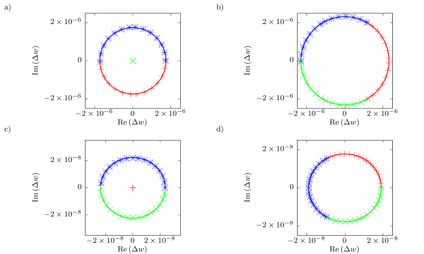
Figure 3: Encircling of the pitchfork bifurcation P1 of the excited state (a) in the complex scattering length $a$ with the radius $r_{a}=10^{-5}$ and (b) in the complex asymmetry parameter $s$ with the radius $r_{s}=10^{-5}$. The permutation of only two states in (a) and all three states in (b) is clearly exhibited. (c) and (d): Same results for the pitchfork bifurcation P2 of the ground state with $r_{a}=1.5\times 10^{-5}$ and $r_{s}=10^{-6}$, respectively. The results of the matrix model (solid lines) agree perfectly with the exact data (symbols).

Obviously, the figure does not show the permutation of three states, which is typical for a cubic-root branching singularity of an EP3. Rather, only the two states emerging in the bifurcation permute, which is the scenario discussed in [15] for the special case that the condition (31) is not fulfilled. Nevertheless, the typical permutation of three states is observed when the asymmetry parameter $s$ is varied along the path of equation (33) with radius $r_{s}=10^{-5}$. By following this path the values of the operator $w$ show the permutation plotted in figure 3(b). All three states permute in the way as expected for an EP3 [11] and discussed in [15] for the generic case that the condition (31) is fulfilled. The different permutation behaviour for both control parameters becomes evident in the matrix model introduced in section 3.3. For $s=0$ the matrix element $P_{31}$ of the perturbation in equation (26) vanishes and thus a square root behaviour is expected for two of the eigenvalues [15], i.e. one eigenvalue is constant, $\Delta w_{1}=0$, and two eigenvalues follow the paths $\Delta w_{2,3}\sim\rme^{{\rm k}\varphi/2}$ and permute after one circle around the exceptional point. When the exceptional point is encircled in the complex $s$ parameter, the condition $P_{31}\neq 0$ is fulfilled, and the three eigenvalues are $\Delta w_{j}\sim\rme^{{\rm k}\varphi/3}$, resulting in the typical permutation of all three states as expected for an EP3.

The pitchfork bifurcation P2 occurring in the ground state for an ansatz with $N=6$ coupled Gaussian functions can be analysed in the same way and exhibits a similar behaviour as the bifurcation of the excited state. For the path in the scattering length (equation (32)) with radius $r_{a}=1.5\times 10^{-5}$ encircling the bifurcation at $a_{\rm P2}=-0.0036$ the values of the operator $w$ show the permutation of two states (see figure 3(c)). However, if the asymmetry parameter $s$ follows the path given in equation (33) with $r_{s}=10^{-6}$ all three states permute as shown in figure 3(d).

As already discussed above, the mean-field energy near the points P1 and P2 in figure 2 does not show the typical level splittings expected for a pitchfork bifurcation, and this is also true when the exceptional points are encircled. The analysis of the matrix model $Q_{E}$ for the mean-field energy in equation (28) reveals that two eigenvalues $\Delta E_{\rm mf}$ follow a path $\sim\rme^{2{\rm k}\varphi}$ when the exceptional point is encircled in the scattering length $a$, i.e. one circle in the scattering length results in two loops in the mean-field energy. When the exceptional point is encircled in the asymmetry parameter $s$ all three mean-field energies follow paths $\sim\rme^{{\rm k}(4/3)\varphi}$, which, however, also means a permutation of all three states after one circle in $s$.

4.2 Two parameter perturbations

In the previous sections we examined situations where only one of the parameters $s$ or $a-a_{\rm cr}$ is nonzero. We now investigate perturbations of the pitchfork bifurcations where both parameters are nonzero. Results where either $s$ or $a-a_{\rm cr}$ is set to a constant nonzero value and the other parameter is varied are presented in figure 4.

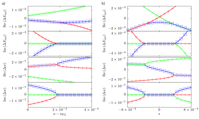
Figure 4: Level splittings $\Delta E$ and $\Delta w$ for two parameter perturbations of the pitchfork bifurcation P2. In (a) the cylindrical symmetry of the trap is broken with $s=-10^{-3}$. In (b) the scattering length is chosen such that $a-a_{\rm P2}=9.35\times 10^{-5}$. The symbols mark the results obtained using an ansatz of six Gaussian functions and agree perfectly with the solid lines obtained with the linear matrix model.

In figure 4(a) the symmetry of the trap is broken by setting $s=-10^{-3}$. The pitchfork bifurcation does no longer exist and only a tangent bifurcation between two states remains, as schematically illustrated in figure 1(b). The typical square root behaviour of a tangent bifurcation can be clearly seen in the real part of $\Delta w$ in figure 4(a), the branch below the bifurcation point of the tangent bifurcation belongs to complex eigenvalues and is obtained only with the analytic continuation of the GPE. In figure 4(b) the scattering length is set to a constant value $a=a_{\rm P2}+9.35\times 10^{-5}$ and the asymmetry parameter $s$ is varied. Here, the pitchfork bifurcation is replaced with two tangent bifurcations located at $s=\pm 3.6\times 10^{-4}$. Three real states exist in the region between the two tangent bifurcations, outside that range there are one real and two complex states.

The symbols in figure 4 mark the results of the GPE obtained with a variational approach using six coupled Gaussian functions. They are in excellent agreement with the results of the matrix model (26) for the expectation values $w=\langle\psi|x^{2}-y^{2}|\psi\rangle$ and the matrix model (28) for the mean-field energy. The perfect agreement even for the two parameter perturbations is remarkable since both matrix models only use two adjustable parameters to describe the level splittings in equations (19) and (20), which have been determined solely with the data of the one parameter perturbations. Similar results as shown in figure 4 for the two parameter perturbations of the pitchfork bifurcation P2 of the ground state are also obtained (but not shown) for the pitchfork bifurcation P1 of the excited state.

How do the exceptional points related to the pitchfork bifurcations behave under the two parameter perturbations? In order to answer this question we follow different parameter paths marked C1 to C3 in figure 5 either in the complex scattering length plane for a constant value $s\neq 0$ (see figure 5(a)) or in the complex $s$ plane for a constant value $a\neq a_{\rm cr}$ (see figure 5(b)).

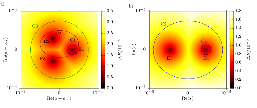
Figure 5: Two parameter perturbations of the pitchfork bifurcation P1 using an ansatz with a single Gaussian function and the trap parameters $\bar{\gamma}_{1}=34000$ and $\lambda_{1}=6$. In (a) the axial symmetry of the trap is broken with $s=10^{-4}$, and in (b) the scattering length is $a-a_{\rm P1}=2\times 10^{-5}$. (c) Illustrations of the composed permutations of the states when one, two, or three exceptional points are encircled along the paths C1 to C3, respectively.

For each path we observe a different permutation behaviour of the three states, which can be explained as follows. The colours (or gray values) in figure 5(a) and (b) indicate the minimal distance (absolute value) between the mean-field energies of the three states, i.e. a zero value means the coalescence of at least two states. In figure 5(a) three points where two states coalesce are revealed. The point marked E1 is a tangent bifurcation point on the real $a$ axis, as already discussed (see figures 1(b) and 4(a)). The points E2 and E3 are new points in the imaginary half planes of the scattering length where different state pairs coalesce. If each point is encircled separately they show the permutation behaviour of an EP2 where the two participating states permute. Following the path C2 which encircles E1 and E2 the cyclic permutation of all three states is observed. If all points E1 to E3 are encircled along the path C3, we find the same permutation behaviour as for the pitchfork bifurcation of the dipolar BEC in an axisymmetric trap, i.e. two states permute. The splitting of the EP3 of the pitchfork bifurcation into three EP2 for the broken trap symmetry can only be observed in the permutation behaviour of the states if a path is chosen which does not include all three points E1 to E3. The points E1 to E3 in figure 5(a) merge at $a=a_{\rm cr}$ in the limit $s\to 0$ of the asymmetry parameter.

The results in the complex $s$ plane for constant scattering length $a>a_{\rm cr}$ are presented in figure 5(b). Here, the pitchfork bifurcation point P1 is split into the two tangent bifurcation points E4 and E5. If the two points are encircled separately each of them shows the permutation of two states typical of an EP2. If they are encircled together along the path C2 in figure 5(b) the cyclic permutation of all three states as in figure 3(b) is observed, i.e. the typical behaviour of an EP3. As in figure 5(a) the splitting of the EP3 into two exceptional points with a square root behaviour can only be observed if a path is chosen which does not include both points E4 and E5, and these points merge at $s=0$ in the limit $a\to a_{\rm cr}$.

The possible permutations of states when one, two, or three exceptional points are encircled by a path C1, C2, or C3 is illustrated in figure 5(c). The combinations produce the same permutation behaviour for two and three EPs as discussed in [21].

The exceptional points observed in figure 5(a) and (b) can also be obtained with the matrix model in equation (26) or (28). The eigenvalues of the traceless matrices $Q_{w}$ or $Q_{E}$ are the roots of the characteristic polynomial $\chi(\lambda)=\lambda^{3}+p\lambda+q$. Two eigenvalues are degenerate when the discriminant $D=4p^{3}+27q^{2}$ vanishes. This yields the condition

$$4\tilde{a}^{3}=4c_{a}^{3}(a-a_{\rm cr})^{3}=27s^{2}$$ (34)

for the scattering length and the asymmetry parameter. For a constant value $s\neq 0$ equation (34) provides one real and two complex solutions for EP2 exceptional points in the complex $a$ plane, which agree with the points E1 to E3 marked in figure 5(a). For a given value $a\neq a_{\rm cr}$ of the scattering length equation (34) provides two real or two imaginary solutions for $s$, which coincide with the exceptional points E4 and E5 in figure 5(b).

5 Summary

When dipolar BECs are described within a mean-field theory the GPE exhibits a rich variety of nonlinear phenomena including tangent and pitchfork bifurcations of states and the occurrence of exceptional points. We have solved the GPE with an extended variational approach using coupled Gaussian functions, and presented a method to find all states participating in the pitchfork bifurcations, including the complex branches, which have been obtained by analytic continuation of the GPE using bicomplex numbers. We have analysed in detail the various bifurcations between the states depending on two parameters, viz. the scattering length $a$ and the parameter $s$ breaking the axial symmetry of the harmonic trap. The origin of the bifurcations is the nonlinearity of the GPE, nevertheless, the mean-field energies $E_{\rm mf}$ and the expectation values $w=\langle\psi|x^{2}-y^{2}|\psi\rangle$ of the states participating in the pitchfork bifurcations can be excellently described by a linear model with non-Hermitian matrices.

Both the variational computations and the linear model have been used to investigate the properties of the exceptional points. At the bifurcation points of a pitchfork bifurcation not only the three eigenvalues but also the eigenvectors coincide, indicating the existence of an EP3. However, a different behaviour for the permutation of states is observed when the exceptional point is encircled either in the complex continued scattering length $a$ or in the asymmetry parameter $s$. The structures resemble those obtained in a linear model using perturbation theory for non-Hermitian operators [15].

For two parameter perturbations the pitchfork bifurcation is split into either three or two tangent bifurcations located in the complex $a$ or $s$ parameter plane, respectively. The typical signature of an EP2 is obtained when a single exceptional point is encircled. Paths surrounding two or three exceptional points yield the behaviour of combined permutations [21].

The results presented in this article need not be restricted to dipolar condensates. Rather, the signatures of exceptional points related to pitchfork bifurcations discussed here for dipolar condensates may be generic features of nonlinear systems with pitchfork bifurcations, however, further investigations will be necessary to clarify this point. We also expect the results of our investigations to arouse the interest of experimentalists to search for experimental evidences of the appearance of exceptional points in Bose-Einstein condensates.

Appendix A Integrals for the variational ansatz

The ansatz (7) with coupled Gaussians for the wave functions requires the calculation of Gaussian integrals to set up the linear system of equations (10). The integrals can be computed analytically or with the help of elliptic integrals. With the abbreviations

$$a_{\sigma}^{kl}=A_{\sigma}^{k}+(A_{\sigma}^{l})^{*}\;,\leavevmode\nobreak\ a_{\sigma}^{klij}=a_{\sigma}^{kl}+a_{\sigma}^{ij}\;\leavevmode\nobreak\ {\rm with}\leavevmode\nobreak\ \leavevmode\nobreak\ \sigma=x,y,z\;,$$ (35)

$$\gamma^{kl}=\gamma^{k}+(\gamma^{l})^{*}\;,\leavevmode\nobreak\ \gamma^{klij}=\gamma^{kl}+\gamma^{ij}\;,\leavevmode\nobreak\$$ (36)

$$\kappa_{x}^{klij}=\sqrt{\frac{a_{x}^{klij}a_{z}^{ij}a_{z}^{kl}}{a_{x}^{ij}a_{x}^{kl}a_{z}^{klij}}}\;,\leavevmode\nobreak\ \kappa_{y}^{klij}=\sqrt{\frac{a_{y}^{klij}a_{z}^{ij}a_{z}^{kl}}{a_{y}^{ij}a_{y}^{kl}a_{z}^{klij}}}$$ (37)

the integrals read

$$\langle g^{l}|g^{k}\rangle =\frac{\pi^{3/2}\rme^{-\gamma^{kl}}}{\sqrt{a_{x}^{kl}a_{y}^{kl}a_{z}^{kl}}}\;,$$ (38)

$$\langle g^{l}|x^{2}|g^{k}\rangle =\frac{\pi^{3/2}\rme^{-\gamma^{kl}}}{2\left(a_{x}^{kl}\right)^{3/2}\sqrt{a_{y}^{kl}a_{z}^{kl}}}\;,$$ (39)

$$\langle g^{l}|x^{4}|g^{k}\rangle =\frac{3\pi^{3/2}\rme^{-\gamma^{kl}}}{4\left(a_{x}^{kl}\right)^{5/2}\sqrt{a_{y}^{kl}a_{z}^{kl}}}\;,$$ (40)

$$\langle g^{l}|x^{2}y^{2}|g^{k}\rangle =\frac{\pi^{3/2}\rme^{-\gamma^{kl}}}{4\left(a_{x}^{kl}a_{y}^{kl}\right)^{3/2}\sqrt{a_{z}^{kl}}}\;,$$ (41)

$$\langle g^{l}|V_{\rm c}|g^{k}\rangle =8a\pi^{5/2}\sum_{i,j=1}^{N}\frac{\rme^{-\gamma^{klij}}}{\sqrt{a_{x}^{klij}a_{y}^{klij}a_{z}^{klij}}}\;,$$ (42)

$$\langle g^{l}|x^{2}V_{\rm c}|g^{k}\rangle =4a\pi^{5/2}\sum_{i,j=1}^{N}\frac{\rme^{-\gamma^{klij}}}{\left(a_{x}^{klij}\right)^{3/2}\sqrt{a_{y}^{klij}a_{z}^{klij}}}\;,$$ (43)

$$\langle g^{l}|V_{\rm d}|g^{k}\rangle =\frac{4\pi^{5/2}}{3}\sum_{i,j=1}^{N}\frac{\rme^{-\gamma^{klij}}}{\sqrt{a_{x}^{klij}a_{y}^{klij}a_{z}^{klij}}}\left[\kappa_{x}\kappa_{y}R_{D}\left(\kappa_{x}^{2},\kappa_{y}^{2},1\right)-1\right]\;,$$ (44)

$$\langle g^{l}|x^{2}V_{\rm d}|g^{k}\rangle =\frac{4\pi^{5/2}}{3}\sum_{i,j=1}^{N}\frac{\rme^{-\gamma^{klij}}}{\sqrt{a_{x}^{klij}a_{y}^{klij}a_{z}^{klij}}}\Bigg{[}\frac{1}{2a_{x}^{klij}}\left(\kappa_{x}\kappa_{y}R_{D}\left(\kappa_{x}^{2},\kappa_{y}^{2},1\right)-1\right)$$ (45)

$$\phantom{=\;}-\bigg{(}\left(\kappa_{y}R_{D}\left(\kappa_{x}^{2},\kappa_{y}^{2},1\right)+2\kappa_{x}^{2}\kappa_{y}R_{x}\left(\kappa_{x}^{2},\kappa_{y}^{2},1\right)\right)\frac{\partial\kappa_{x}}{\partial A_{x}^{k}}$$

$$\phantom{=\;}-\left(\kappa_{x}R_{D}\left(\kappa_{x}^{2},\kappa_{y}^{2},1\right)+2\kappa_{x}\kappa_{y}^{2}R_{y}\left(\kappa_{x}^{2},\kappa_{y}^{2},1\right)\right)\frac{\partial\kappa_{y}}{\partial A_{x}^{k}}\bigg{)}\Bigg{]}\;,$$

$$\langle g^{l}|y^{2}V_{\rm d}|g^{k}\rangle =\frac{4\pi^{5/2}}{3}\sum_{i,j=1}^{N}\frac{\rme^{-\gamma^{klij}}}{\sqrt{a_{x}^{klij}a_{y}^{klij}a_{z}^{klij}}}\Bigg{[}\frac{1}{2a_{y}^{klij}}\left(\kappa_{x}\kappa_{y}R_{D}\left(\kappa_{x}^{2},\kappa_{y}^{2},1\right)-1\right)$$ (46)

$$\phantom{=\;}-\bigg{(}\left(\kappa_{y}R_{D}\left(\kappa_{x}^{2},\kappa_{y}^{2},1\right)+2\kappa_{x}^{2}\kappa_{y}R_{x}\left(\kappa_{x}^{2},\kappa_{y}^{2},1\right)\right)\frac{\partial\kappa_{x}}{\partial A_{y}^{k}}$$

$$\phantom{=\;}-\left(\kappa_{x}R_{D}\left(\kappa_{x}^{2},\kappa_{y}^{2},1\right)+2\kappa_{x}\kappa_{y}^{2}R_{y}\left(\kappa_{x}^{2},\kappa_{y}^{2},1\right)\right)\frac{\partial\kappa_{y}}{\partial A_{y}^{k}}\bigg{)}\Bigg{]}\;,$$

$$\langle g^{l}|z^{2}V_{\rm d}|g^{k}\rangle =\frac{4\pi^{5/2}}{3}\sum_{i,j=1}^{N}\frac{\rme^{-\gamma^{klij}}}{\sqrt{a_{x}^{klij}a_{y}^{klij}a_{z}^{klij}}}\Bigg{[}\frac{1}{2a_{z}^{klij}}\left(\kappa_{x}\kappa_{y}R_{D}\left(\kappa_{x}^{2},\kappa_{y}^{2},1\right)-1\right)$$ (47)

$$\phantom{=\;}-\bigg{(}\left(\kappa_{y}R_{D}\left(\kappa_{x}^{2},\kappa_{y}^{2},1\right)+2\kappa_{x}^{2}\kappa_{y}R_{x}\left(\kappa_{x}^{2},\kappa_{y}^{2},1\right)\right)\frac{\partial\kappa_{x}}{\partial A_{z}^{k}}$$

$$\phantom{=\;}-\left(\kappa_{x}R_{D}\left(\kappa_{x}^{2},\kappa_{y}^{2},1\right)+2\kappa_{x}\kappa_{y}^{2}R_{y}\left(\kappa_{x}^{2},\kappa_{y}^{2},1\right)\right)\frac{\partial\kappa_{y}}{\partial A_{z}^{k}}\bigg{)}\Bigg{]}\;.$$

In equations (44)-(47) the upper indices at $\kappa_{x}^{klij}$ and $\kappa_{y}^{klij}$ have been omitted. The elliptic integrals $R_{D}(x,y,z)$ are given in equation (15), and their derivatives are defined as

$$R_{x}(x,y,z)=\partial_{x}R_{D}(x,y,z)\;,\;R_{y}(x,y,z)=\partial_{y}R_{D}(x,y,z)\;.$$ (48)

Integrals of the harmonic trap $V_{\rm t}$ are easily obtained with the equations given above. Integrals not given above are obtained by appropriate permutations of $x$, $y$ and $z$.

References

References

- [1] M. H. Anderson, J. R. Ensher, M. R. Matthews, C. E. Wieman, and E. A. Cornell. Observation of Bose-Einstein condensation in a dilute atomic vapor. Science, 269:198, 1995.
- [2] C. C. Bradley, C. A. Sackett, J. J. Tollett, and R. G. Hulet. Evidence of Bose-Einstein condensation in an atomic gas with attractive interactions. Phys. Rev. Lett., 75:1687, 1995.
- [3] K. B. Davis, M. O. Mewes, M. R. Andrews, N. J. van Druten, D. S. Durfee, D. M. Kurn, and W. Ketterle. Bose-Einstein condensation in a gas of sodium atoms. Phys. Rev. Lett., 75:3969, 1995.
- [4] T. Lahaye, C. Menotti, L. Santos, M. Lewenstein, and T. Pfau. The physics of dipolar bosonic quantum gases. Rep. Prog. Phys., 72:126401, 2009.
- [5] D. O’Dell, S. Giovanazzi, G. Kurizki, and V. M. Akulin. Bose-Einstein condensates with interatomic attraction: Electromagnetically induced “gravity”. Phys. Rev. Lett., 84:5687, 2000.
- [6] I. Papadopoulos, P. Wagner, G. Wunner, and J. Main. Bose-Einstein condensates with attractive interaction: The case of self-trapping. Phys. Rev. A, 76:053604, 2007.
- [7] H. Cartarius, J. Main, and G. Wunner. Discovery of exceptional points in the Bose-Einstein condensation of gases with attractive interaction. Phys. Rev. A, 77:013618, 2008.
- [8] T. Kato. Perturbation theory for linear operators. Springer, Berlin, 1966.
- [9] W. D. Heiss and A. L. Sannino. Avoided level crossings and exceptional points. J. Phys. A, 23:1167, 1990.
- [10] W. D. Heiss. Phase of wave functions and level repulsion. Eur. Phys. J. D, 7:1, 1999.
- [11] W. D. Heiss. Chirality of wavefunctions for three coalescing levels. J. Phys. A: Math. Theor., 41:244010, 2008.
- [12] W. D. Heiss. The physics of exceptional points. J. Phys. A: Math. Theor., 45:444016, 2012.
- [13] P. Köberle, H. Cartarius, T. Fabčič, J. Main, and G. Wunner. Bifurcations, order and chaos in the Bose–Einstein condensation of dipolar gases. New J. Phys., 11:023017, 2009.
- [14] S. Rau, J. Main, P. Köberle, and G. Wunner. Pitchfork bifurcations in blood-cell-shaped dipolar Bose-Einstein condensates. Phys. Rev. A, 81:031605(R), 2010.
- [15] G. Demange and E.-M. Graefe. Signatures of three coalescing eigenfunctions. J. Phys. A: Math. Theor., 45:025303, 2012.
- [16] S. Rau, J. Main, and G. Wunner. Variational methods with coupled Gaussian functions for Bose-Einstein condensates with long-range interactions. I. General concept. Phys. Rev. A, 82:023610, 2010.
- [17] S. Rau, J. Main, H. Cartarius, P. Köberle, and G. Wunner. Variational methods with coupled Gaussian functions for Bose-Einstein condensates with long-range interactions. II. Applications. Phys. Rev. A, 82:023611, 2010.
- [18] A. D. McLachlan. A variational solution of the time-dependent Schrödinger equation. Mol. Phys., 8:39, 1964.
- [19] B. C. Carlson. Numerical computation of real or complex elliptic integrals. Numerical Algorithms, 10:13, 1995.
- [20] T. Koch, T. Lahaye, J. Metz, B. Fröhlich, A. Griesmaier, and T. Pfau. Stabilizing a purely dipolar quantum gas against collapse. Nature Physics, 4:218–222, 2008.
- [21] J.-W. Ryu, S.-Y. Lee, and S. W. Kim. Analysis of multiple exceptional points related to three interacting eigenmodes in a non-Hermitian Hamiltonian. Phys. Rev. A, 85:042101, 2012.