TUM-HEP 877/13

UCI-TR-2013-03

FLAVOUR(267104)-ERC-36

CETUP*-12/018

Predictivity of models with spontaneously broken non–Abelian discrete flavor symmetries

Mu–Chun Chen

Department of Physics and Astronomy, University of California,
  Irvine, California 92697–4575, USA

Maximilian Fallbacher, Yuji Omura, Michael Ratz, Christian Staudt

Physik Department T30, Technische Universität München,
  James–Franck–Straße, 85748 Garching, Germany

In a class of supersymmetric flavor models predictions are based on residual symmetries of some subsectors of the theory such as those of the charged leptons and neutrinos. However, the vacuum expectation values of the so–called flavon fields generally modify the Kähler potential of the setting, thus changing the predictions. We derive simple analytic formulae that allow us to understand the impact of these corrections on the predictions for the masses and mixing parameters. Furthermore, we discuss the effects on the vacuum alignment and on flavor changing neutral currents. Our results can also be applied to non–supersymmetric flavor models.

1 Introduction

Explanations of the observed pattern of fermion masses and mixing are often based on spontaneously broken flavor symmetries. In this paper, we concentrate on supersymmetric models attempting to explain the observed flavor structure by discrete symmetries. At some (high) energy scale, the flavor symmetry, denoted by $G_{\mathrm{F}}$ in what follows, is spontaneously broken by some appropriate ‘flavon’ fields, which acquire vacuum expectation values (VEVs). Although our analysis also applies to non–supersymmetric settings, we base our discussion on the lepton sector of supersymmetric extensions of the standard model (SM). In order to be specific, consider a prototype superpotential of the form

$$\mathscr{W}_{\mathrm{leading}}~{}=~{}\frac{1}{\Lambda}({\Phi_{e}})_{gf}\,L^{g}\,R^{f}\,H_{d}+\frac{1}{\Lambda\,\Lambda_{\nu}}({\Phi_{\nu}})_{gf}\,L^{g}\,H_{u}\,L^{f}\,H_{u}\;,$$ (1.1)

where $L^{g}$ and $R^{f}$ (with the flavor indices $1\leq f,g\leq 3$) denote the lepton doublets and singlets, respectively, whereas $H_{u}$ and $H_{d}$ are the usual Higgs doublets of the supersymmetric standard model. The two scales involved are the cut–off scale $\Lambda$ of the theory and the see–saw scale $\Lambda_{\nu}$. For the sake of definiteness, we shall take $\Lambda$ to be around the unification scale, although our results will not depend on this choice. $\Phi_{e}$ and $\Phi_{\nu}$ denote the flavons, which acquire VEVs that are assumed to be somewhat below $\Lambda$ such that the expansion parameters of our theory are $\langle\Phi_{e}\rangle/\Lambda$ and $\langle\Phi_{\nu}\rangle/\Lambda$. Inserting the flavon VEVs leads to an effective superpotential

$$\mathscr{W}_{\mathrm{eff}}~{}=~{}(Y_{e})_{gf}\,L^{g}\,R^{f}\,H_{d}+\frac{1}{4}\kappa_{gf}\,L^{g}\,H_{u}\,L^{f}\,H_{u}\;.$$ (1.2)

One is often left with a situation in which neither $\Phi_{e}$ nor $\Phi_{\nu}$ breaks $G_{\mathrm{F}}$ completely, but respect the residual symmetries $G_{\mathrm{e}}$ and $G_{\nu}$, respectively (cf. figure 1), while the intersection of the residual symmetries is smaller or empty. Given that higher–order terms are either subleading or may be completely forbidden by some appropriate symmetries such as $R$ symmetries, these residual symmetries allow us to make predictions.

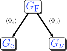
Figure 1: The flavor symmetry $G_{\mathrm{F}}$ gets broken to different subgroups in different sectors of the theory.

Models that make predictions based on such residual symmetries have become rather popular in the past (see e.g. [1, 2]). One can, for example, successfully obtain the bi–maximal mixing pattern [3, 4] as well as the tri–bi–maximal (TBM) mixing pattern [5, 6].

The potential problem with such predictions is that they are based on the holomorphic superpotential only. However, there are modifications coming from the Kähler potential [7, 8, 9]. Given the fact that for most of the proposed patterns the mixing parameters, i.e. mixing angles and phases, run under the renormalization group (RG), and that in supersymmetric theories RG corrections affect the Kähler potential only, it is clear that it will be nearly impossible to avoid such corrections. One may, therefore, question how solid the predictions based only on the holomorphic sector really are. Clearly, the canonical Kähler potential does not include all terms allowed by the flavor symmetry. Rather, if one is to derive predictions from higher–order terms in the expansion parameters $\langle\Phi_{e/\nu}\rangle/\Lambda$, one should take into account both the superpotential and the Kähler potential. The full Kähler potential is

$$K~{}=~{}K_{\mathrm{canonical}}+\Delta K\;,$$ (1.3)

where the canonical part is given by (only considering the leptons)

$$K_{\mathrm{canonical}}~{}\supset~{}\left(L^{f}\right)^{\dagger}\,\delta_{fg}\,L^{g}+\left(R^{f}\right)^{\dagger}\,\delta_{fg}\,R^{g}\;.$$ (1.4)

$\Delta K$ includes contractions of $L^{f}$ and $R^{f}$ with the flavons, such as $(L\Phi_{e/\nu})^{\dagger}(L\Phi_{e/\nu})$, which may not be forbidden by any (conventional) symmetry, and it has the general form

$$\Delta K~{}=~{}\left(L^{f}\right)^{\dagger}\,(\Delta\mathscr{K}_{L})_{fg}\,L^{g}+\left(R^{f}\right)^{\dagger}\,(\Delta\mathscr{K}_{R})_{fg}\,R^{g}\;.$$ (1.5)

Here $\Delta\mathscr{K}_{L}$ and $\Delta\mathscr{K}_{R}$ are Hermitean matrices which describe the modification of the Kähler metric after the flavons acquire their VEVs. The structure of these Hermitean matrices, therefore, depends on the flavor group and the flavon VEVs.

After the breaking of the flavor symmetry, one needs to redefine the fields in order to return to a canonical Kähler potential [10, 11, 12]. As we shall discuss in more detail below, in this new basis generically none of the subsectors exhibits a residual symmetry. Among other things, this explains why the parameters run even though their values appear to be determined by $G_{\mathrm{e}}$ and $G_{\nu}$, respectively. The crucial property of $\Delta K$ is that its size will, in general, be controlled by the above expansion parameters $\langle\Phi_{e}\rangle/\Lambda$ and $\langle\Phi_{\nu}\rangle/\Lambda$, i.e. the very same quantities that set the scale of the entries of the mass and coupling matrices in the effective superpotential $\mathscr{W}_{\mathrm{eff}}$. In addition, $\Delta K$ will depend on Kähler coefficients which multiply the above contractions and are hard to determine in an effective field theory approach.

Using methods previously used for the renormalization group equations (RGEs) in [13, 14], one can obtain an analytic understanding of the Kähler corrections [15, 16, 17]. As we pointed out in [17], the corresponding corrections are sizable and will in general lead to a strong modification of the predictions. In particular, they may render patterns that appeared to be ruled out, such as the TBM one, consistent with observation — and vice versa.

The purpose of this paper is to extend our discussion of these changes by presenting a full derivation of the analytic formulae. We start out in section 2 by reviewing the predictions from the superpotential of two well–known models, one of which is based on $\mathrm{A}_{4}$ [18] and the other on $\mathrm{T}^{\prime}$ [19], and also compare the results to the current best fit values. In section 3 we provide an analytic discussion of the Kähler corrections. We then apply our analytic understanding to the two sample models in section 4, in which we also comment on the implications of Kähler corrections for the VEV alignment and for flavor changing neutral currents (FCNCs). Finally, section 5 summarizes our results.

2 Mixing parameters from the superpotential

In this section we review by means of two simple examples how predictions based on residual symmetries of the mass terms in the superpotential are derived.

2.1 TBM from $\mathrm{A}_{4}$

One of the simplest and most popular choices of a flavor symmetry group is $\mathrm{A}_{4}$ [6]. The resulting mixing is characterized by the TBM mixing matrix

$$U_{\mathrm{TBM}}~{}=~{}\begin{pmatrix}\sqrt{\frac{2}{3}}&\frac{1}{\sqrt{3}}&0\\ -\frac{1}{\sqrt{6}}&\frac{1}{\sqrt{3}}&-\frac{1}{\sqrt{2}}\\ -\frac{1}{\sqrt{6}}&\frac{1}{\sqrt{3}}&\frac{1}{\sqrt{2}}\end{pmatrix}\;,$$ (2.1)

which leads to the mixing angles in standard parametrization (cf. appendix A.1) shown in table 2.1.

	$\theta_{12}$	$\theta_{13}$	$\theta_{23}$
TBM prediction:	$\arctan{\left(\sqrt{0.5}\right)}\approx 35.3^{\circ}$	$0$	$45^{\circ}$
Best fit values $(\pm 1\sigma)$:	$\left(33.6^{+1.1}_{-1.0}\right)^{\circ}$	$\left(8.93^{+0.46}_{-0.48}\right)^{\circ}$	$\left(38.4^{+1.4}_{-1.2}\right)^{\circ}$

Table 2.1: Tri–bi–maximal prediction for the neutrino mixing angles and best fit values from the global fit by [20].

The measurement of $\theta_{13}$ [21, 22, 23] revealed a considerable deviation from the tri–bi–maximal prediction and also the recent best fit values from global analyses for $\theta_{23}$ are in tension with maximal mixing. Yet, the TBM pattern may still serve as a good first order approximation of the observed mixing angles.

As common to many flavor models, the three generations of left–handed lepton doublets are assumed to transform as a triplet under $\mathrm{A}_{4}$, $L\sim$ $\boldsymbol{3}$. The three singlet representations of $\mathrm{A}_{4}$, $\boldsymbol{1}$, $\boldsymbol{1^{\prime\prime}}$ and $\boldsymbol{1^{\prime}}$, are assigned to the right–handed charged leptons $e_{\mathrm{R}}$, $\mu_{\mathrm{R}}$ and $\tau_{\mathrm{R}}$, respectively, and the Higgs fields $H_{u}$ and $H_{d}$ are not charged under the flavor symmetry. The mass matrices are generated by VEVs of three flavon fields: the two $\mathrm{A}_{4}$ triplets ${\Phi_{\nu}}$ and ${\Phi_{e}}$, and the pure singlet $\xi\sim$ $\boldsymbol{1}$. At leading order in the ratio flavon VEV over the cut–off scale, the terms leading to the Yukawa couplings and to the Weinberg neutrino operator (cf. equation (1.1)) read

$$\mathscr{W}_{\nu} = \frac{\lambda_{1}}{\Lambda\,\Lambda_{\mathrm{\nu}}}\,\left\{\left[(L\,H_{u})\otimes(L\,H_{u})\right]_{\boldsymbol{3}_{\mathrm{s}}}\otimes{\Phi_{\nu}}\right\}_{\boldsymbol{1}}+\frac{\lambda_{2}}{\Lambda\,\Lambda_{\mathrm{\nu}}}\,\left[(L\,H_{u})\otimes(L\,H_{u})\right]_{\boldsymbol{1}}\,\xi\;,$$ (2.2)

$$\mathscr{W}_{e} = \frac{h_{e}}{\Lambda}\,\left({\Phi_{e}}\otimes L\right)_{\boldsymbol{1}}\,H_{d}\,e_{\mathrm{R}}+\frac{h_{\mu}}{\Lambda}\,\left({\Phi_{e}}\otimes L\right)_{\boldsymbol{1^{\prime}}}\,H_{d}\,\mu_{\mathrm{R}}+\frac{h_{\tau}}{\Lambda}\,\left({\Phi_{e}}\otimes L\right)_{\boldsymbol{1^{\prime\prime}}}\,H_{d}\,\tau_{\mathrm{R}}\;,$$ (2.3)

where again $\Lambda$ and $\Lambda_{\nu}$ denote the cut–off and the see–saw scale, respectively.

In order to distinguish the flavon field ${\Phi_{\nu}}$, which couples to the neutrinos, from the flavon field ${\Phi_{e}}$, which couples to the charged leptons, one introduces an additional $\mathbbm{Z}_{4}$ symmetry. Under this symmetry, ${\Phi_{\nu}}$ changes sign whereas ${\Phi_{e}}$ stays invariant. Furthermore, under the $\mathbbm{Z}_{4}$ symmetry, $\xi\rightarrow-\xi$, $L\rightarrow\mathrm{i}L$ and $R\rightarrow-\mathrm{i}R$.

The desired tri–bi–maximal lepton mixing is achieved when the flavons acquire VEVs in the directions

$$\langle{\Phi_{\nu}}\rangle = \left(v,v,v\right)\;,$$ (2.4a)

$$\langle{\Phi_{e}}\rangle = \left(v^{\prime},0,0\right)\;,$$ (2.4b)

$$\langle\xi\rangle = w\;.$$ (2.4c)

This choice breaks the flavor symmetry $G_{\mathrm{F}}=\mathrm{A}_{4}\times\mathbbm{Z}_{4}$ to $G_{\mathrm{e}}=\mathbbm{Z}_{3}\times\mathbbm{Z}_{4}$ and $G_{\nu}=\mathbbm{Z}_{2}\times\mathbbm{Z}_{2}$ in the charged lepton and neutrino sector, respectively. These residual symmetries lead to TBM. This can be seen explicitly by computing the mass matrices after electroweak symmetry breaking. The charged lepton mass matrix reads

$$m_{e}~{}=~{}v_{d}\,\operatorname{diag}\left(y_{e},\,y_{\mu},\,y_{\tau}\right)\;,$$ (2.5)

where $v_{d}$ is the VEV of the down–type Higgs and $y_{e,\,\mu,\,\tau}=h_{e,\,\mu,\,\tau}\,\frac{v^{\prime}}{\Lambda}$. Here and in the following we work in a basis in which the charged lepton Yukawa matrix is diagonal.

On the other hand, in this basis the neutrino mass matrix is non–diagonal. Using the abbreviations $a=2\lambda_{2}\,\frac{v_{u}^{2}}{\Lambda_{\mathrm{\nu}}}\,\frac{w}{\Lambda}$ and $d=\sqrt{2}\lambda_{1}\,\frac{v_{u}^{2}}{\Lambda_{\nu}}\,\frac{v}{\Lambda}$, where $v_{u}$ is the VEV of the up–type Higgs, it can be written as

$$m_{\nu}~{}=~{}\begin{pmatrix}a+2d&-d&-d\\ -d&2d&a-d\\ -d&a-d&2d\end{pmatrix}\;.$$ (2.6)

The lepton mixing matrix $U_{\mathrm{PMNS}}$ is then the unitary transformation that diagonalizes the neutrino mass matrix and is indeed given by the tri–bi–maximal matrix (2.1).

Even though this simple model seems to be excluded by the recent measurements, there are still many loopholes which can make it viable. For example, there are attempts to explain the deviations by higher–order terms in the superpotential, cf. [24] and references therein. However, as we have shown in [17], there are also corrections due to higher–order Kähler potential terms, which can either reconcile the model predictions with data or drive them even further away.

2.2 $\mathrm{T}^{\prime}$

Another interesting example model is based on the double covering group of $\mathrm{A}_{4}$, which is called $\mathrm{T}^{\prime}$. Like $\mathrm{A}_{4}$, this group contains three irreducible singlet representations and one triplet. Additionally, the group contains three doublet representations $\boldsymbol{2}$, $\boldsymbol{2^{\prime}}$ and $\boldsymbol{2^{\prime\prime}}$. The specific model [19] we discuss comes with several flavon fields, which are summarized in table 2.2, and also two additional Abelian $\mathbbm{Z}_{12}$ symmetries.

	$\phi$	$\phi^{\prime}$	$\psi$	$\psi^{\prime}$	$\zeta$	$N$	$\xi$	$\eta$
$\mathrm{T}^{\prime}$	$\boldsymbol{3}$	$\boldsymbol{3}$	$\boldsymbol{2^{\prime}}$	$\boldsymbol{2}$	$\boldsymbol{1^{\prime\prime}}$	$\boldsymbol{1^{\prime}}$	$\boldsymbol{3}$	$\boldsymbol{1}$
$\mathbbm{Z}_{12}$	3	2	6	9	9	3	10	10
$\mathbbm{Z}_{12}$	3	6	7	8	2	11	0	0

Table 2.2: Flavon content of the $\mathrm{T}^{\prime}$ model.

The flavons acquire VEVs along the directions

$$\langle\phi\rangle = \phi_{0}\,\left(\begin{array}[]{c}1\\ 0\\ 0\end{array}\right)\;,\quad\langle\phi^{\prime}\rangle~{}=~{}\phi^{\prime}_{0}\left(\begin{array}[]{c}1\\ 1\\ 1\end{array}\right)\;,\quad\langle\xi\rangle~{}=~{}\xi_{0}\,\left(\begin{array}[]{c}1\\ 1\\ 1\end{array}\right)\;,$$ (2.16)

$$\langle\psi\rangle = \psi_{0}\,\left(\begin{array}[]{c}1\\ 0\end{array}\right)\;,\quad\langle\psi^{\prime}\rangle~{}=~{}\psi^{\prime}_{0}\,\left(\begin{array}[]{c}1\\ 1\end{array}\right)\;,$$ (2.21)

and the fields transforming as one–dimensional representations, $\zeta$, $N$ and $\eta$, assume non–trivial values. With this choice of VEVs, the model [19] gives rise to near tri–bi–maximal lepton mixing,

$$\theta_{12}~{}\approx~{}33^{\circ}\;,\quad\theta_{23}~{}=~{}45^{\circ}\quad\text{and}\quad\theta_{13}~{}\approx~{}3^{\circ}\;.$$ (2.22)

The deviations from the exact TBM mixing pattern are due to the corrections from the charged lepton sector, and they are related to the Cabibbo angle through the $\mathrm{SU}(5)$ GUT relations. Furthermore, the model also predicts a leptonic Dirac CP violating phase from the superpotential and an absolute neutrino mass scale, e.g. $m_{1}=0.0156\,\text{e\kern-0.59998ptV}$ for mass–squared differences given by $\Delta m_{21}^{2}~{}=~{}8.0\cdot 10^{-5}\,(\text{e\kern-0.59998ptV})^{2}$ and $\Delta m_{32}^{2}~{}=~{}2.4\cdot 10^{-3}\,(\text{e\kern-0.59998ptV})^{2}$.

3 Corrections due to Kähler potential terms

Let us now look at the Kähler potential of the theory. As already mentioned, higher–order terms will, after the flavons acquire their VEVs, lead to a non–canonical Kähler metric. Let us spell this out in more detail, using the $\mathrm{A}_{4}$ and the $\mathrm{T}^{\prime}$ examples from section 2. Here, the left–handed lepton doublets transform as a triplet of either $\mathrm{A}_{4}$ or $\mathrm{T}^{\prime}$, respectively. Contractions of these triplets with the flavons will then lead to a Kähler metric with off–diagonal terms after the flavons acquire a VEV.

3.1 Linear flavon corrections from left–handed leptons

We start with terms which are linear in the flavons. Focussing on the $\mathrm{A}_{4}$ symmetry only, these linear contributions are given by

$$\Delta K_{\mathrm{linear}}~{}=~{}\sum\limits_{i\,\in\{\mathrm{a},\mathrm{s}\}}\left(\frac{\kappa_{{\Phi_{\nu}}}^{(i)}}{\Lambda}\,{L^{\dagger}\,(L\otimes{\Phi_{\nu}})_{\boldsymbol{3}_{i}}}+\frac{\kappa_{{\Phi_{e}}}^{(i)}}{\Lambda}\,{L^{\dagger}\,(L\otimes{\Phi_{e}})_{\boldsymbol{3}_{i}}}\right)+\frac{\kappa_{\xi}}{\Lambda}\,{\xi\,L^{\dagger}L}+\text{h.c.}\;,$$ (3.1)

and are suppressed by only one power of the expansion parameter $\langle\Phi_{e/\nu}\rangle/\Lambda$. The last term does not lead to a change of the mixing parameters because it just changes the overall normalization of the kinetic term of the lepton doublets. On the other hand, the terms containing ${\Phi_{\nu}}$ and ${\Phi_{e}}$ do modify the model predictions. The contractions with a generic triplet flavon $\Phi$ are

$${L^{\dagger}\,(L\otimes\Phi)_{\boldsymbol{3}_{\mathrm{s}}}} = \frac{1}{\sqrt{2}}\,\left[(L_{1}^{\dagger})(2\,L_{1}\Phi_{1}-L_{2}\Phi_{3}-L_{3}\Phi_{2})\right.+(L_{2}^{\dagger})(2\,L_{3}\Phi_{3}-L_{1}\Phi_{2}-L_{2}\Phi_{1})$$ (3.2a)

$${}\hphantom{\frac{1}{\sqrt{2}}\,\left[\right.}+\left.(L_{3}^{\dagger})(2\,L_{2}\Phi_{2}-L_{1}\Phi_{3}-L_{3}\Phi_{1})\right]\;,$$

$${L^{\dagger}\,(L\otimes\Phi)_{\boldsymbol{3}_{\mathrm{a}}}} = \mathrm{i}\,\sqrt{\frac{3}{2}}\,\left[(L_{1}^{\dagger})(L_{2}\Phi_{3}-L_{3}\Phi_{2})\right.+(L_{2}^{\dagger})(L_{1}\Phi_{2}-L_{2}\Phi_{1})$$ (3.2b)

$${}\hphantom{\mathrm{i}\,\sqrt{\frac{3}{2}}\,\left[\right.}+\left.(L_{3}^{\dagger})(L_{3}\Phi_{1}-L_{1}\Phi_{3})\right]\;.$$

Plugging in the flavon VEVs leads to departures from the canonical Kähler metric,

$$\mathscr{K}_{fg}~{}=~{}\left(\frac{\partial^{2}K}{\partial(L^{f})^{\dagger}\,\partial L^{g}}\right)~{}=~{}\delta_{fg}~{}\xrightarrow{\Phi\to\langle\Phi\rangle}~{}\delta_{fg}+(\Delta\mathscr{K})_{fg}\;.$$ (3.3)

In what follows, we will find it convenient to decompose $\Delta\mathscr{K}$ according to

$$(\Delta\mathscr{K})_{fg}~{}=~{}\alpha\,P_{fg}+\text{h.c.}\;,$$ (3.4)

where $P$ encodes the matrix structure and $\alpha$ is a continuous parameter reflecting the size of the Kähler correction. For the flavon VEV $\langle\Phi\rangle=\langle{\Phi_{e}}\rangle=(v^{\prime},0,0)$ one obtains the Kähler corrections

$$(\Delta\mathscr{K})_{{\Phi_{e}}}^{(\mathrm{s})} = \kappa_{{\Phi_{e}}}^{(s)}\,v^{\prime}\,\frac{1}{\sqrt{2}}\,P_{{\Phi_{e}}}^{(\mathrm{s})}+\text{h.c.}\;,$$ (3.5a)

$$(\Delta\mathscr{K})_{{\Phi_{e}}}^{(\mathrm{a})} = \mathrm{i}\,\kappa_{{\Phi_{e}}}^{(a)}\,v^{\prime}\,\sqrt{\frac{3}{2}}\,P_{{\Phi_{e}}}^{(\mathrm{a})}+\text{h.c.}$$ (3.5b)

with the $P$ matrices

$$P_{{\Phi_{e}}}^{(\mathrm{s})} = \operatorname{diag}(2,-1,-1)\;,$$ (3.6a)

$$P_{{\Phi_{e}}}^{(\mathrm{a})} = \operatorname{diag}(0,-1,1)\;,$$ (3.6b)

whereas for $\langle\Phi\rangle=\langle{\Phi_{\nu}}\rangle=(v,v,v)$ one gets

$$(\Delta\mathscr{K})_{{\Phi_{\nu}}}^{(\mathrm{s})} = \kappa_{{\Phi_{\nu}}}^{(s)}\,v\,\frac{1}{\sqrt{2}}\,P_{{\Phi_{\nu}}}^{(\mathrm{s})}+\text{h.c.}\;,$$ (3.7a)

$$(\Delta\mathscr{K})_{{\Phi_{\nu}}}^{(\mathrm{a})} = \mathrm{i}\,\kappa_{{\Phi_{\nu}}}^{(a)}\,v\,\sqrt{\frac{3}{2}}\,P_{{\Phi_{\nu}}}^{(\mathrm{a})}+\text{h.c.}$$ (3.7b)

with

$$P_{{\Phi_{\nu}}}^{(\mathrm{s})} = \left(\begin{array}[]{ccc}2&-1&-1\\ -1&-1&2\\ -1&2&-1\end{array}\right)\;,$$ (3.8d)

$$P_{{\Phi_{\nu}}}^{(\mathrm{a})} = \left(\begin{array}[]{ccc}0&1&-1\\ 1&-1&0\\ -1&0&1\end{array}\right)\;.$$ (3.8h)

However, in the specific $\mathrm{A}_{4}$ model from section 2.1, the terms comprising ${\Phi_{\nu}}$ are forbidden by the additional $\mathbbm{Z}_{4}$ symmetry. Therefore, we only get corrections in this case from the matrices in equation (3.6a) and equation (3.6b). One may introduce additional symmetries in such a way that all flavons are charged (like in the $\mathrm{T}^{\prime}$ example in section 2.2), and hence forbid linear flavon contributions in the Kähler potential all together. Therefore, these linear corrections will not necessarily spoil the predictivity of a given model. This is different in the case of quadratic corrections, which we discuss next.

3.2 Second order corrections from left–handed leptons

Unlike the linear terms, some of the quadratic corrections to the Kähler potential, which are of the form $(L\otimes\Phi_{i})^{\dagger}(L\otimes\Phi_{j})$, cannot be forbidden by any (conventional) symmetry. Obviously, terms with $i\neq j$ can again be forbidden by a symmetry, however, terms like $(L\otimes\Phi)^{\dagger}(L\otimes\Phi)$ with $\Phi={\Phi_{\nu}}$ or ${\Phi_{e}}$ cannot. We will comment later in section 5 how one may control or avoid such corrections in more complete settings. In the $\mathrm{A}_{4}$ model we get six different possible terms for each flavon, $(L\otimes{\Phi_{\nu}})_{\boldsymbol{R}}^{\dagger}(L\otimes{\Phi_{\nu}})_{\boldsymbol{R^{\prime}}}$ and $(L\otimes{\Phi_{e}})_{\boldsymbol{R}}^{\dagger}(L\otimes{\Phi_{e}})_{\boldsymbol{R^{\prime}}}$, e.g.  $(L\otimes{\Phi_{\nu}})_{\boldsymbol{3}_{s}}^{\dagger}(L\otimes{\Phi_{\nu}})_{\boldsymbol{3}_{a}}$. Using the $\mathrm{A}_{4}$ multiplication rules from appendix A.2, the latter term can be recast as

$$(L\otimes{\Phi_{\nu}})^{\dagger}_{\boldsymbol{3}_{s}}(L\otimes{\Phi_{\nu}})_{\boldsymbol{3}_{a}}$$ (3.9)

$$= \mathrm{i}\,\frac{\sqrt{3}}{2}\,\left[\left(2\,L_{1}^{\dagger}{\Phi_{\nu}}_{1}^{\dagger}-L_{2}^{\dagger}{\Phi_{\nu}}_{3}^{\dagger}-L_{3}^{\dagger}{\Phi_{\nu}}_{2}^{\dagger}\right)\left(L_{2}{\Phi_{\nu}}_{3}-L_{3}{\Phi_{\nu}}_{2}\right)\right.$$

$${}\hphantom{\mathrm{i}\,\frac{\sqrt{3}}{2}\,\left[\right.}+\left(2L_{3}^{\dagger}{\Phi_{\nu}}_{3}^{\dagger}-L_{2}^{\dagger}{\Phi_{\nu}}_{1}^{\dagger}-L_{1}^{\dagger}{\Phi_{\nu}}_{2}^{\dagger}\right)\left(L_{1}{\Phi_{\nu}}_{2}-L_{2}{\Phi_{\nu}}_{1}\right)$$

$${}\hphantom{\mathrm{i}\,\frac{\sqrt{3}}{2}\,\left[\right.}+\left.\left(2L_{2}^{\dagger}{\Phi_{\nu}}_{2}^{\dagger}-L_{1}^{\dagger}{\Phi_{\nu}}_{3}^{\dagger}-L_{3}^{\dagger}{\Phi_{\nu}}_{1}^{\dagger}\right)\left(L_{3}{\Phi_{\nu}}_{1}-L_{1}{\Phi_{\nu}}_{3}\right)\right]\;$$

and leads to the Kähler correction

$$\Delta\mathscr{K}~{}=~{}\mathrm{i}\,\kappa\,\frac{\sqrt{3}}{2}\,P+\text{h.c.}$$ (3.10)

with the $P$ matrix

$$P~{}=~{}\begin{pmatrix}-{\Phi_{\nu}}_{2}^{\dagger}{\Phi_{\nu}}_{2}+{\Phi_{\nu}}_{3}^{\dagger}{\Phi_{\nu}}_{3}&2{\Phi_{\nu}}_{1}^{\dagger}{\Phi_{\nu}}_{3}+{\Phi_{\nu}}_{2}^{\dagger}{\Phi_{\nu}}_{1}&-2{\Phi_{\nu}}_{1}^{\dagger}{\Phi_{\nu}}_{2}-{\Phi_{\nu}}_{3}^{\dagger}{\Phi_{\nu}}_{1}\\ -2{\Phi_{\nu}}_{2}^{\dagger}{\Phi_{\nu}}_{3}-{\Phi_{\nu}}_{1}^{\dagger}{\Phi_{\nu}}_{2}&-{\Phi_{\nu}}_{3}^{\dagger}{\Phi_{\nu}}_{3}+{\Phi_{\nu}}_{1}^{\dagger}{\Phi_{\nu}}_{1}&2{\Phi_{\nu}}_{2}^{\dagger}{\Phi_{\nu}}_{1}+{\Phi_{\nu}}_{3}^{\dagger}{\Phi_{\nu}}_{2}\\ 2{\Phi_{\nu}}_{3}^{\dagger}{\Phi_{\nu}}_{2}+{\Phi_{\nu}}_{1}^{\dagger}{\Phi_{\nu}}_{3}&-2{\Phi_{\nu}}_{3}^{\dagger}{\Phi_{\nu}}_{1}-{\Phi_{\nu}}_{2}^{\dagger}{\Phi_{\nu}}_{3}&{\Phi_{\nu}}_{2}^{\dagger}{\Phi_{\nu}}_{2}-{\Phi_{\nu}}_{1}^{\dagger}{\Phi_{\nu}}_{1}\end{pmatrix}.$$ (3.11)

We then get for $\langle{\Phi_{\nu}}\rangle=(v,v,v)$

$$\Delta\mathscr{K}~{}=~{}\mathrm{i}\,\frac{\sqrt{3}}{2}\,\kappa\,v^{2}\left(\begin{array}[]{ccc}0&3&-3\\ -3&0&3\\ 3&-3&0\end{array}\right)+\text{h.c.}~{}=~{}3\frac{\sqrt{3}}{2}\,\kappa\,v^{2}\,P_{\mathrm{V}}+\text{h.c.}\;.$$ (3.12)

If we treat all of the possible twelve terms (six for each flavon) in such a way, we get several corrections which lead to identical $P$ matrices. In total, we can summarize them by five different matrices $P_{\mathrm{I}-\mathrm{V}}$, where the derivation of the fifth matrix $P_{\mathrm{V}}$ has just been shown above. The first three matrices

$$P_{\mathrm{I}}~{}=~{}\operatorname{diag}(1,0,0)\;,\quad P_{\mathrm{II}}~{}=~{}\operatorname{diag}(0,1,0)\quad\text{and}\quad P_{\mathrm{III}}~{}=~{}\operatorname{diag}(0,0,1)$$ (3.13a)

come from contractions of $$L {\Phi_{e}} \langle{\Phi_{e}}\rangle=(v^{\prime},0,0) (v^{\prime})^{2}$$ with . Since , their contribution in the Kähler potential is proportional to . The other two matrices,

$$P_{\mathrm{IV}}~{}=~{}\begin{pmatrix}1&1&1\\ 1&1&1\\ 1&1&1\end{pmatrix}\quad\text{and}\quad P_{\mathrm{V}}~{}=~{}\begin{pmatrix}0&\mathrm{i}&-\mathrm{i}\\ -\mathrm{i}&0&\mathrm{i}\\ \mathrm{i}&-\mathrm{i}&0\end{pmatrix}\;,$$ (3.13b)

are contributions due to ${\Phi_{\nu}}$; therefore, their contribution is proportional to $v^{2}$ since $\langle{\Phi_{\nu}}\rangle=(v,v,v)$. An important property of all these corrections is that they are controlled by the square of our expansion parameters VEV over the fundamental scale as well as some unknown coefficient in the Kähler potential.

3.3 Corrections from the right–handed leptons

As was already stated in the introduction one can also have corrections for the right–handed lepton fields, depending on their representation under the flavor group. In the $\mathrm{A}_{4}$ example, the right–handed leptons are $\mathrm{A}_{4}$ singlets, $\boldsymbol{1}$, $\boldsymbol{1^{\prime}}$ and $\boldsymbol{1^{\prime\prime}}$; therefore, corrections with the flavon triplets are going to be diagonal, e.g.

$$K~{}\supset~{}\frac{1}{\Lambda^{2}}\,\left(e_{\mathrm{R}}\,{\Phi_{\nu}}\right)^{\dagger}\left(e_{\mathrm{R}}\,{\Phi_{\nu}}\right)~{}=~{}e_{\mathrm{R}}^{\dagger}\,e_{\mathrm{R}}\,\frac{{\Phi_{\nu}}^{\dagger}\,{\Phi_{\nu}}}{\Lambda^{2}}\;,$$ (3.14)

which, after VEV insertion, gives $3\,|v|^{2}\,e_{\mathrm{R}}^{\dagger}\,e_{\mathrm{R}}/\Lambda^{2}$. We get similar terms for $\mu_{\mathrm{R}}$, $\tau_{\mathrm{R}}$ and also for contractions of the right–handed leptons with the flavon field ${\Phi_{e}}$. The only other flavon in the model is the $\mathrm{A}_{4}$ singlet $\xi$; hence, we also have diagonal corrections proportional to $|\langle\xi\rangle|^{2}$.

The model could also contain flavons which are in the singlet representation $\boldsymbol{1^{\prime}}$ or $\boldsymbol{1^{\prime\prime}}$, in this case, non–diagonal corrections are possible due to terms with two different flavons. However, these corrections, just like the linear ones, can easily be forbidden by an additional symmetry. Therefore, we focus on corrections for the right–handed lepton fields which are diagonal, i.e. $P_{R}=\operatorname{diag}(\alpha_{1},\alpha_{2},\alpha_{3})$ where the $\alpha_{i}$ are not related and depend on the VEVs and arbitrary Kähler coefficients. Since we are working in a basis with diagonal charged lepton Yukawa matrices, a diagonal redefinition of the right–handed fields can only affect the mass eigenvalues but not the mixing angles. This is also reflected by our analytical formulae.

3.4 Second order corrections for a model based on $\mathrm{T}^{\prime}$

We now extend our previous analysis to a model which is based on $\mathrm{T}^{\prime}$ [19], the double covering group of $\mathrm{A}_{4}$. As stated in section 2.2, $\mathrm{T}^{\prime}$, like $\mathrm{A}_{4}$, contains three irreducible one–dimensional representations and one triplet. Beyond this, the multiplication law for the contraction of two triplets is the same. For doublets and triplets, it is given by

$$\boldsymbol{2},\boldsymbol{2^{\prime}},\boldsymbol{2^{\prime\prime}}\otimes\boldsymbol{3}~{}=~{}\boldsymbol{2}\oplus\boldsymbol{2^{\prime}}\oplus\boldsymbol{2^{\prime\prime}}\;.$$ (3.15)

A complete list of tensor products can be found, for instance, in [25]. A closer look at table 2.2 shows that in this model there are no linear corrections in the Kähler potential, since all flavons are charged under one of the $\mathbbm{Z}_{12}$ symmetries. Nonetheless, there are several second order corrections: looking at the VEV structure of the flavon fields in equation (2.21), it is obvious that we have the same Kähler corrections as in the $\mathrm{A}_{4}$ example due to the flavons $\phi$, $\phi^{\prime}$ and $\xi$. However, there are additional terms due to the doublet fields $\psi$ and $\psi^{\prime}$ through higher–order terms of the form $\left(L\otimes\psi\right)_{\boldsymbol{R}}^{\dagger}\left(L\otimes\psi\right)_{\boldsymbol{R}}$ and $\left(L\otimes\psi^{\prime}\right)_{\boldsymbol{R}}^{\dagger}\left(L\otimes\psi^{\prime}\right)_{\boldsymbol{R}}$. The contributions of these terms can be determined with the multiplication law in equation (3.15), which shows that $\boldsymbol{R}$ can only be one of the three doublets. Using this multiplication rule, we get, e.g., the contribution

$$\left(L\otimes\psi^{\prime}\right)_{\boldsymbol{2^{\prime}}}^{\dagger}\left(L\otimes\psi^{\prime}\right)_{\boldsymbol{2^{\prime}}} = \left(\sqrt{2}\,\psi^{\prime}_{2}\,L_{3}+\psi^{\prime}_{1}\,L_{2}\right)^{\dagger}\left(\sqrt{2}\,\psi^{\prime}_{2}\,L_{3}+\psi^{\prime}_{1}\,L_{2}\right)+$$ (3.16)

$$+ \left(\sqrt{2}\,\psi^{\prime}_{1}\,L_{1}-\psi^{\prime}_{2}\,L_{2}\right)^{\dagger}\left(\sqrt{2}\,\psi^{\prime}_{1}\,L_{1}-\psi^{\prime}_{2}\,L_{2}\right)\;,$$

which results in the Kähler correction

$$\Delta\mathscr{K}~{}=~{}\kappa_{\boldsymbol{2^{\prime}2^{\prime}}}\,\,\left(\begin{array}[]{ccc}2\,(\psi^{\prime}_{1})^{2}&-\sqrt{2}\,(\psi^{\prime}_{1})^{\dagger}\,\psi^{\prime}_{2}&0\\ -\sqrt{2}\,\psi^{\prime}_{1}\,(\psi^{\prime}_{2})^{\dagger}&(\psi^{\prime}_{1})^{2}+(\psi^{\prime}_{2})^{2}&\sqrt{2}\,(\psi^{\prime}_{1})^{\dagger}\,\psi^{\prime}_{2}\\ 0&\sqrt{2}\,\psi^{\prime}_{1}\,(\psi^{\prime}_{2})^{\dagger}&2\,(\psi^{\prime}_{2})^{2}\end{array}\right)+\text{h.c.}\;.$$ (3.17)

After inserting the VEV $\langle\psi^{\prime}\rangle=\left(\psi^{\prime}_{0},\,\psi^{\prime}_{0}\right)^{T}$, we get $\Delta\mathscr{K}~{}=~{}\kappa_{\boldsymbol{2^{\prime}2^{\prime}}}\,(\psi^{\prime}_{0}/\Lambda)^{2}\,P+\text{h.c.}$ with

$$P~{}=~{}\left(\begin{array}[]{ccc}2&-\sqrt{2}&0\\ -\sqrt{2}&2&\sqrt{2}\\ 0&\sqrt{2}&2\end{array}\right)\;.$$ (3.18)

Summarizing, the $\mathrm{T}^{\prime}$ model admits the same corrections as in the $\mathrm{A}_{4}$ case, described in equation (3.13a) and equation (3.13b), and in addition corrections proportional to the $P$ matrices

$$P_{\mathsf{i}}~{}=~{}\operatorname{diag}(0,2,1)\;,\quad P_{\mathsf{ii}}~{}=~{}\operatorname{diag}(1,0,2)\quad\text{and}\quad P_{\mathsf{iii}}~{}=~{}\operatorname{diag}(2,1,0)$$ (3.19a)

coming from contractions of $$L \psi \langle\psi\rangle=(\psi_{0},0) (\psi_{0})^{2}$$ with . Since , their contribution in the Kähler potential is proportional to . Furthermore, Kähler corrections proportional to the three matrices

$$P_{\mathsf{iv}} = \begin{pmatrix}2&\sqrt{2}&-\sqrt{2}\\ \sqrt{2}&2&0\\ -\sqrt{2}&0&2\end{pmatrix}\;,\quad P_{\mathsf{v}}~{}=~{}\begin{pmatrix}2&0&\sqrt{2}\\ 0&2&-\sqrt{2}\\ \sqrt{2}&-\sqrt{2}&2\end{pmatrix}\quad\text{and}$$

$$P_{\mathsf{vi}} = \begin{pmatrix}2&-\sqrt{2}&0\\ -\sqrt{2}&2&\sqrt{2}\\ 0&\sqrt{2}&2\end{pmatrix}\;,$$ (3.19b)

are all due to contractions with $\psi^{\prime}$. Since $\langle\psi^{\prime}\rangle=(\psi^{\prime}_{0},\psi^{\prime}_{0})$, their contribution is proportional to $(\psi^{\prime}_{0})^{2}$.

3.5 General $\boldsymbol{P}$ matrices

In the general case of different flavon VEVs, or possibly a different symmetry group, one can imagine that not all Kähler correction matrices $P$ can be expressed as linear combinations of the $P_{i}$ in equations (3.13) and (3.19). Therefore, there are in general more possible $P$ matrices. However, since the Kähler corrections are Hermitean, one can express a general $P$ matrix in terms of nine Hermitean basis matrices,

$$P_{1}~{}=~{}\begin{pmatrix}1&0&0\\ 0&0&0\\ 0&0&0\end{pmatrix}\;,\quad P_{2}~{}=~{}\begin{pmatrix}0&1&0\\ 1&0&0\\ 0&0&0\end{pmatrix}\;,\quad P_{3}~{}=~{}\begin{pmatrix}0&0&0\\ 0&1&0\\ 0&0&0\end{pmatrix}\;,$$ (3.20a)

$$P_{4}~{}=~{}\begin{pmatrix}0&0&1\\ 0&0&0\\ 1&0&0\end{pmatrix}\;,\quad P_{5}~{}=~{}\begin{pmatrix}0&0&0\\ 0&0&1\\ 0&1&0\end{pmatrix}\;,\quad P_{6}~{}=~{}\begin{pmatrix}0&0&0\\ 0&0&0\\ 0&0&1\end{pmatrix}\;,$$ (3.20b)

$$P_{7}~{}=~{}\begin{pmatrix}0&-\mathrm{i}&0\\ \mathrm{i}&0&0\\ 0&0&0\end{pmatrix}\;,\quad P_{8}~{}=~{}\begin{pmatrix}0&0&-\mathrm{i}\\ 0&0&0\\ \mathrm{i}&0&0\end{pmatrix}\;,\quad P_{9}~{}=~{}\begin{pmatrix}0&0&0\\ 0&0&-\mathrm{i}\\ 0&\mathrm{i}&0\end{pmatrix}\;.$$ (3.20c)

Then, e.g., the $P$ matrices in equations (3.13) of our $\mathrm{A}_{4}$ example can be expressed as

$$P_{\mathrm{I}}~{}=~{}P_{1}\;,\quad P_{\mathrm{II}}~{}=~{}P_{3}\;,\quad P_{\mathrm{III}}~{}=~{}P_{6}\;,\quad P_{\mathrm{IV}}~{}=~{}\sum_{i=1}^{6}P_{i}\;,\quad P_{\mathrm{V}}~{}=~{}\sum_{i=7}^{9}(-1)^{i}\,P_{i}\;,$$ (3.21)

respectively.

3.6 Analytic formulae for Kähler corrections

In this section, we give a detailed account of the derivation of analytical formulae for the corrections to the mixing parameters coming from the Kähler potential, building on earlier publications [26, 16].

3.6.1 The general idea

Let us start by specifying the goal of our derivation. We assume that we are given a model that makes predictions for the leptonic mixing parameters without taking into account any terms in the Kähler potential beside the canonical ones. That is, the superpotential alone predicts the lepton masses, mixing angles and complex phases, and the Kähler potential has the form shown in equation (1.4). We emphasize that it is irrelevant for the following computations how precisely the prediction for the parameters of the lepton sector is achieved. In principle, we only need the charged lepton Yukawa matrix and the Majorana neutrino mass matrix as input. Furthermore, for computational simplicity, we assume that the model has been transformed to a basis where the charged lepton Yukawa matrix is diagonal. Hence, a complete set of input parameters is given by the three charged lepton masses, the three neutrino masses and the nine mixing parameters, which we assume to be in the standard parametrization (cf. appendix A.1).

After having specified the input, we now consider the same model but amended with correction terms in the Kähler potential. That is, we allow for an arbitrary Kähler potential for the left–handed lepton doublets $L=(L_{1},L_{2},L_{3})$ and the right–handed lepton singlets $R=(R_{1},R_{2},R_{3})$,

$$K~{}\supset~{}L^{\dagger}\,\mathscr{K}_{L}\,L+R^{\dagger}\,\mathscr{K}_{R}\,R\;,$$ (3.22)

with the Hermitean matrices

$$\mathscr{K}_{L/R}~{}=~{}\mathbbm{1}+\Delta\mathscr{K}_{L/R}\;.$$ (3.23)

Because of the corrections $\Delta\mathscr{K}_{L/R}$, $L$ and $R$ are not canonically normalized. Since $\mathscr{K}_{L/R}$ are Hermitean and positive, they can be rewritten as

$$\mathscr{K}_{L/R}~{}=~{}H_{L/R}^{\dagger}H_{L/R}~{}=~{}H_{L/R}^{2}\\$$ (3.24)

with Hermitean $H_{L/R}=H_{L/R}^{\dagger}$, such that the canonically normalized fields are

$$L^{\prime} = H_{L}\,L\;,$$ (3.25a)

$$R^{\prime} = H_{R}\,R\;.$$ (3.25b)

Since we assume the Kähler corrections $\Delta\mathscr{K}_{L/R}$ to arise from terms that are suppressed with respect to the canonical terms by powers of the flavon VEVs over the fundamental scale, we specialize to infinitesimal $\Delta\mathscr{K}_{L/R}$,

$$\Delta\mathscr{K}_{L} = -2\,x_{1}\,P_{L}\;,$$ (3.26a)

$$\Delta\mathscr{K}_{R} = -2\,x_{2}\,P_{R}\;.$$ (3.26b)

Here $P_{L}$ and $P_{R}$ are Hermitean, $x_{1}$ and $x_{2}$ are infinitesimal, and the factors $-2$ turn out to be convenient. The goal of the following discussion is to find analytic formulae for the dependence of the mixing parameters on $x_{1}$ and $x_{2}$ for generic $P_{L/R}$.

Before we go on with the discussion, a comment is in order. We assume that the lepton basis is chosen such that the charged lepton Yukawa matrix is diagonal with positive real entries. However, this does not fix the basis completely since one can still perform a phase redefinition of the left–handed and right–handed lepton fields without changing the Yukawa matrix as long as the phase change is the same for both sectors. This freedom is conventionally used to absorb the three so–called unphysical phases $\delta_{e}$, $\delta_{\mu}$ and $\delta_{\tau}$ of $U_{\mathrm{PMNS}}$ into the fields. However, this is only possible for a diagonal Kähler potential. In the non–diagonal case discussed here, this redefinition also changes $P_{L/R}$ according to

$$P_{L/R}\rightarrow\widehat{P}_{L/R}~{}=~{}U_{\mathrm{ph}}^{\dagger}\,P_{L/R}\,U_{\mathrm{ph}}\;,$$ (3.27)

where $U_{\mathrm{ph}}=\operatorname{diag}{(e^{\mathrm{i}\delta_{e}},e^{\mathrm{i}\delta_{\mu}},e^{\mathrm{i}\delta_{\tau}})}$ is a diagonal matrix containing the unphysical phases. That is, after setting the unphysical phases to zero in the mixing matrix, the transformed $\widehat{P}_{L/R}$ depends on them. This shows explicitly that the changes in the mixing parameters depend on the values of $\delta_{e}$, $\delta_{\mu}$ and $\delta_{\tau}$. Our results are derived for the case in which the three phases in $U_{\mathrm{PMNS}}$ are zero at $x_{1}=x_{2}=0$. If this is not the case, one has to apply the resulting formulae not to the original $P_{L/R}$ but to $\widehat{P}_{L/R}$ as defined in equation (3.27).

For the following discussion, it turns out to be useful to introduce for any unitary matrix $U$ a corresponding anti–Hermitean matrix

$$T~{}:=~{}U^{\dagger}U^{\prime}\;,$$ (3.28)

where the prime denotes the derivative with respect to $x_{1}$ or $x_{2}$ (it will be clear from the context which one is meant), such that

$$U^{\prime}~{}=~{}U\,T\,.$$ (3.29)

Hence, for the leptonic mixing matrix $U_{\mathrm{PMNS}}$, we define

$$T_{\mathrm{PMNS}}~{}:=~{}U_{\mathrm{PMNS}}^{\dagger}\,U_{\mathrm{PMNS}}^{\prime}\;.$$ (3.30)

Since $T_{\mathrm{PMNS}}$ is anti–Hermitean, it has nine independent real parameters

$$u~{}:=~{}\left\{\operatorname{Re}T_{12},\operatorname{Re}T_{13},\operatorname{Re}T_{23},\operatorname{Im}T_{11},\operatorname{Im}T_{12},\operatorname{Im}T_{13},\operatorname{Im}T_{22},\operatorname{Im}T_{23},\operatorname{Im}T_{33}\right\}\;.$$ (3.31)

On the other hand, one can use the definition of $T_{\mathrm{PMNS}}$, i.e. equation (3.30), in order to express its entries in terms of the mixing parameters and their derivatives. Clearly, $T_{\mathrm{PMNS}}$ is linear in the derivatives of the mixing parameters. Therefore, there is a linear map $A$ from the derivatives of the mixing parameters to the elements of $T_{\mathrm{PMNS}}$, which only depends on the mixing parameters but not on their derivatives. Defining

$$\xi~{}:=~{}\{\theta_{12}^{\prime},\theta_{13}^{\prime},\theta_{23}^{\prime},\delta^{\prime},\delta_{e}^{\prime},\delta_{\mu}^{\prime},\delta_{\tau}^{\prime},\varphi_{1}^{\prime},\varphi_{2}^{\prime}\}\;,$$ (3.32)

one can write this relation in matrix form,

$$A\,\xi~{}=~{}u\;.$$ (3.33)

The first steps of our computation are to compute $u$ in terms of the mixing parameters, then to read off $A$ from this expression and finally to invert $A$. This way one obtains linear differential equations for the mixing parameters. The remaining task is to find $T_{\mathrm{PMNS}}$ for arbitrary given Kähler corrections $P_{L/R}$.

One can split this task into several parts. First, one can make use of the definition of $U_{\mathrm{PMNS}}:=U_{e}^{\dagger}U_{\nu}$ in order to split the derivative $U^{\prime}_{\mathrm{PMNS}}$ into two parts,

$$U^{\prime}_{\mathrm{PMNS}}~{}=~{}(U_{e}^{\prime})^{\dagger}U_{\nu}+U_{e}^{\dagger}U_{\nu}^{\prime}\,.$$ (3.34)

Multiplying this with $U_{\mathrm{PMNS}}^{\dagger}$ from the left and inserting twice an identity matrix yields

$$T_{\mathrm{PMNS}}~{}=~{}U_{\mathrm{PMNS}}^{\dagger}\,(U_{e}^{\prime})^{\dagger}\,(U_{e}U_{e}^{\dagger})\,U_{\nu}+U_{\mathrm{PMNS}}^{\dagger}\,U_{e}^{\dagger}\,(U_{\nu}U_{\nu}^{\dagger})\,U_{\nu}^{\prime}\;.$$ (3.35)

This can be further simplified by the introduction of the matrices $T_{e}=U_{e}^{\dagger}U_{e}^{\prime}$ and $T_{\nu}=U_{\nu}^{\dagger}U_{\nu}^{\prime}$ and because of the anti–Hermiticity of $T_{e}$ one finally arrives at

$$T_{\mathrm{PMNS}}~{}=~{}T_{\nu}-U_{\mathrm{PMNS}}^{\dagger}\,T_{e}\,U_{\mathrm{PMNS}}\;.$$ (3.36)

In the following, we compute the different contributions to $T_{\nu}$ and $T_{e}$ at $x_{1}=x_{2}=0$. All quantities are from now on evaluated at this point if not indicated otherwise by displaying the arguments $(x_{1})$ or $(x_{2})$ explicitly.

3.6.2 Corrections due to $U_{\nu}$

Let us first discuss the case of $T_{\nu}$. Going to canonically normalized fields by the transformation shown in equation (3.25) leads to the change of the neutrino mass matrix

$$\mathscr{W}_{\nu} = \frac{1}{2}L^{T}\,m_{\nu}^{0}\,L$$ (3.37)

$$\simeq \frac{1}{2}\left[\left(\mathbbm{1}+x_{1}\,P_{L}\right)\,L^{\prime}\right]^{T}\,m_{\nu}^{0}\,\left[\left(\mathbbm{1}+x_{1}\,P_{L}\right)\,L^{\prime}\right]$$

$$\simeq \frac{1}{2}L^{\prime\,T}\,m_{\nu}^{0}\,L^{\prime}+\frac{1}{2}x_{1}\,L^{\prime\,T}\,\left(P_{L}^{T}\,m_{\nu}^{0}+m_{\nu}^{0}\,P_{L}\right)\,L^{\prime}$$

in linear order in $x_{1}$. That is, the change of $m_{\nu}$ is governed by a differential equation which has the same form as the renormalization group equation (RGE) for the neutrino mass operator (cf. equation (B.5) of [13]),

$$\frac{\mathrm{d}}{\mathrm{d}x_{1}}m_{\nu}(x_{1})~{}=~{}P^{T}\,m_{\nu}^{0}+m_{\nu}^{0}\,P\;,\qquad m_{\nu}(0)=m_{\nu}^{0}\;.$$ (3.38)

Therefore, we can repeat the steps in [13] that have led to the analytic solutions to the RGEs for the mixing parameters.

The $x_{1}$–dependent unitary diagonalization matrix $U_{\nu}(x_{1})$ of the neutrino mass matrix $m_{\nu}(x_{1})$ is defined by the equation,

$$U_{\nu}(x_{1})^{T}\,m_{\nu}(x_{1})\,U_{\nu}(x_{1})~{}=~{}D_{\nu}(x_{1})~{}=~{}\operatorname{diag}\left(m_{1}(x_{1}),m_{2}(x_{1}),m_{3}(x_{1})\right)\;,$$ (3.39)

where the mass eigenvalues $m_{i}(x_{1})$ are positive real numbers.

Taking the derivative of equation (3.39) with respect to $x_{1}$, which is denoted by a prime in the following, and evaluating the result at $x_{1}=0$, we obtain

$$\frac{\mathrm{d}}{\mathrm{d}x_{1}}\left(U_{\nu}^{*}(x_{1})\,D_{\nu}(x_{1})\,U_{\nu}^{\dagger}(x_{1})\right)|_{x_{1}=0} = (U_{\nu}^{\prime})^{*}\,D_{\nu}\,U_{\nu}^{\dagger}+U_{\nu}^{*}\,D_{\nu}\,(U_{\nu}^{\prime})^{\dagger}+U_{\nu}^{*}\,D_{\nu}^{\prime}\,U_{\nu}^{\dagger}$$ (3.40)

$$= P_{L}^{T}\,U_{\nu}^{*}\,D_{\nu}\,U_{\nu}^{\dagger}+U_{\nu}^{*}\,D_{\nu}\,U_{\nu}^{\dagger}\,P_{L}\;.$$

All quantities on the right–hand side are evaluated at $x_{1}=0$. Multiplying this equation by $U_{\nu}^{T}$ from the left and by $U_{\nu}$ from the right yields

$$U_{\nu}^{T}\,(U_{\nu}^{\prime})^{*}\,D_{\nu}+D_{\nu}\,(U_{\nu}^{\prime})^{\dagger}\,U_{\nu}+D_{\nu}^{\prime}~{}=~{}\widetilde{P}_{L}^{T}\,D_{\nu}+D_{\nu}\,\widetilde{P}_{L}$$ (3.41)

with

$$\widetilde{P}_{L}~{}=~{}U_{\nu}^{\dagger}\,P_{L}\,U_{\nu}~{}=~{}U_{\mathrm{PMNS}}^{\dagger}\,P_{L}\,U_{\mathrm{PMNS}}\;,$$ (3.42)

where we used the fact that $U_{e}(0,0)=\mathbbm{1}$. With the previously defined anti–Hermitean matrix $T_{\nu}=U_{\nu}^{\dagger}U_{\nu}^{\prime}$ one can rewrite this equation as

$$D_{\nu}^{\prime}~{}=~{}\widetilde{P}_{L}^{T}\,D_{\nu}+D_{\nu}\,\widetilde{P}_{L}-T_{\nu}^{*}\,D_{\nu}+D_{\nu}\,T_{\nu}\;.$$ (3.43)

Since the left–hand side of this equation is diagonal and real, the right–hand side has to have these properties as well and one obtains

$$m_{i}^{\prime}~{}=~{}2\,(\widetilde{P}_{L})_{ii}\,m_{i}+\bigl{(}(T_{\nu})_{ii}-(T_{\nu}^{*})_{ii}\bigr{)}\,m_{i}\;.$$ (3.44)

The first term is real since $P_{L}$ (and thus $\widetilde{P}_{L}$) is Hermitean, whereas the second term is purely imaginary and has to vanish,

$$\operatorname{Im}(T_{\nu})_{ii}~{}=~{}0\;.$$ (3.45)

By comparing the off–diagonal terms one gets

$$m_{i}\,(T_{\nu})_{ij}-(T_{\nu})_{ij}^{*}\,m_{j}~{}=~{}-(\widetilde{P}_{L}^{T})_{ij}\,m_{j}-m_{i}\,(\widetilde{P}_{L})_{ij}$$ (3.46)

such that

$$\operatorname{Re}(T_{\nu})_{ij} = -\frac{m_{j}\,\operatorname{Re}(\widetilde{P}_{L})_{ji}+m_{i}\,\operatorname{Re}(\widetilde{P}_{L})_{ij}}{m_{i}-m_{j}}~{}=~{}-\frac{m_{i}+m_{j}}{m_{i}-m_{j}}\,\operatorname{Re}(\widetilde{P}_{L})_{ij}\;,$$ (3.47a)

$$\operatorname{Im}(T_{\nu})_{ij} = -\frac{m_{j}\,\operatorname{Im}(\widetilde{P}_{L})_{ji}+m_{i}\,\operatorname{Im}(\widetilde{P}_{L})_{ij}}{m_{i}+m_{j}}~{}=~{}-\frac{m_{i}-m_{j}}{m_{i}+m_{j}}\,\operatorname{Im}(\widetilde{P}_{L})_{ij}\;.$$ (3.47b)

This, together with (3.45), specifies all entries of $T_{\nu}$.

3.6.3 Corrections due to $U_{e}$

We turn now to corrections coming from the charged lepton sector. The Yukawa coupling term changes due to the redefinition of the fields as given in equation (3.25),

$$\mathscr{W}_{e} = -R^{T}\,Y_{e}^{0}\,L+\mathrm{h.c.}$$ (3.48)

$$= -R^{\prime\,T}\,\left((H_{R})^{-1}\right)^{T}\,Y_{e}^{0}\,(H_{L})^{-1}\,L^{\prime}+\mathrm{h.c.}$$

$$\simeq -R^{\prime\,T}\,(\mathbbm{1}+x_{2}\,(P_{R})^{T})\,Y_{e}^{0}\,(\mathbbm{1}+x_{1}\,P_{L})\,L^{\prime}+\mathrm{h.c.}$$

$$\simeq -R^{\prime\,T}\,(Y_{e}^{0}+x_{2}\,(P_{R})^{T}\,Y_{e}^{0}+x_{1}\,Y_{e}^{0}\,P_{L})\,L^{\prime}+\mathrm{h.c.}\;.$$

The Yukawa matrix can be diagonalized by a bi–unitary transformation. The matrix $U_{e}$ acting on the left–handed charged leptons is determined to first order in $x_{1}$ and $x_{2}$ by

$$U_{e}^{\dagger}(x_{1},x_{2})\,\left[(Y_{e}^{0})^{2}+2\,x_{2}\,Y_{e}^{0}\,(P_{R})^{T}\,Y_{e}^{0}+x_{1}\,(Y_{e}^{0})^{2}\,P_{L}+x_{1}\,P_{L}\,(Y_{e}^{0})^{2}\right]U_{e}(x_{1},x_{2})\\ =~{}D_{e}^{2}(x_{1},x_{2})~{}=~{}\operatorname{diag}{(y_{1}^{2}(x_{1},x_{2}),y_{2}^{2}(x_{1},x_{2}),y_{3}^{2}(x_{1},x_{2}))}\;,$$ (3.49)

where $D_{e}^{2}(x_{1},x_{2})$ is the diagonal matrix of the squared lepton Yukawa couplings and $D_{e}^{2}(0,0)=(Y_{e}^{0})^{2}$.

We first focus on the $x_{1}$–dependence. Hence, we take the derivative of equation (3.49) with respect to $x_{1}$ and evaluate the resulting expression at $x_{1}=0$, $x_{2}=0$ (remember that $U_{e}(0,0)=\mathbbm{1}$),

$$\frac{\mathrm{d}}{\mathrm{d}x_{1}}\left(U_{e}(x_{1})\,D_{e}^{2}(x_{1})\,U_{e}^{\dagger}(x_{1})\right)|_{x_{1}=0} = U_{e}^{\prime}\,(Y_{e}^{0})^{2}+(Y_{e}^{0})^{2}\,(U_{e}^{\prime})^{\dagger}+(D_{e}^{2})^{\prime}$$ (3.50)

$$= P_{L}\,(Y_{e}^{0})^{2}+(Y_{e}^{0})^{2}\,P_{L}\;.$$

Using the fact that $T_{e}^{x_{1}}=U_{e}^{\prime}$ (where the superscript $x_{1}$ on $T_{e}^{x_{1}}$ means that it is the part of $T_{e}$ which corresponds to changes of $x_{1}$) is anti–Hermitean, one can rearrange this equation into

$$(D_{e}^{2})^{\prime}~{}=~{}P_{L}\,(Y_{e}^{0})^{2}+(Y_{e}^{0})^{2}\,P_{L}-T_{e}^{x_{1}}\,(Y_{e}^{0})^{2}+(Y_{e}^{0})^{2}\,T_{e}^{x_{1}}\;.$$ (3.51)

For the terms on the diagonal this reads

$$(y_{i}^{2})^{\prime}~{}=~{}2\,(P_{L})_{ii}\,y_{i}^{2}\;.$$ (3.52)

There is one important difference from the case of $U_{\nu}$. The diagonal terms $(T_{e}^{x_{1}})_{ii}$ cancel exactly; hence, they cannot be determined from this equation. However, they only contribute to the changes of the unphysical phases which can, after diagonalizing the Kähler potential, be transformed away. Therefore, changes of these phases are of no interest to us. Contrary to the diagonal terms, the off–diagonal terms of $T_{e}^{x_{1}}$ can be derived from equation (3.51),

$$(T_{e}^{x_{1}})_{ij}=(P_{L})_{ij}\,\frac{y_{i}^{2}+y_{j}^{2}}{y_{j}^{2}-y_{i}^{2}}\;.$$ (3.53)

This fixes the first part of $T_{e}^{x_{1}}$ up to the imaginary parts of the entries on the diagonal.

Moreover, there is the part of $T_{e}$ which comes from changes in $x_{2}$, denoted by $T_{e}^{x_{2}}$. Besides the fact that the derivatives are now taken with respect to $x_{2}$, the only difference compared to equation (3.51) is that $P_{L}\,(Y_{e}^{0})^{2}+(Y_{e}^{0})^{2}\,P_{L}$ is replaced by $2\,Y_{e}^{0}\,(P_{R})^{T}\,Y_{e}^{0}$, i.e.

$$(D_{e}^{2})^{\prime}~{}=~{}2\,Y_{e}^{0}\,(P_{R})^{T}\,Y_{e}^{0}-T_{e}^{x_{2}}\,(Y_{e}^{0})^{2}+(Y_{e}^{0})^{2}\,T_{e}^{x_{2}}\;.$$ (3.54)

From this equation one can derive the change of the masses,

$$(y_{i}^{2})^{\prime}~{}=~{}2\,(P_{R})_{ii}\,y_{i}^{2}\;,$$ (3.55)

which again leaves the terms on the diagonal of $T_{e}^{x_{2}}$ undetermined, and the off–diagonal terms of $T_{e}^{x_{2}}$,

$$(T_{e}^{x_{2}})_{ij}=2\,(P_{R})_{ji}\,\frac{y_{i}\,y_{j}}{y_{j}^{2}-y_{i}^{2}}\;.$$ (3.56)

This determines $T_{e}^{x_{2}}$ up to the entries on the diagonal.

Combining all three contributions yields

$$T_{\mathrm{PMNS}}^{x_{1}} = -U_{\mathrm{PMNS}}^{\dagger}\,T_{e}^{x_{1}}\,U_{\mathrm{PMNS}}+T_{\nu}\;,$$ (3.57a)

$$T_{\mathrm{PMNS}}^{x_{2}} = -U_{\mathrm{PMNS}}^{\dagger}\,T_{e}^{x_{2}}\,U_{\mathrm{PMNS}}\;.$$ (3.57b)

From this, one can derive the derivatives of the mixing parameters at $x_{1}=0$, $x_{2}=0$ from which the change of the parameters can be computed to first order by simple multiplication with $x_{1}$ and $x_{2}$, respectively.

3.7 Mathematica package

The formulae that we obtained by following the procedure outlined above are made available online as a Mathematica package. It can be found on the web–page

http://einrichtungen.ph.tum.de/T30e/codes/KaehlerCorrections/.

The package contains the full analytic formulae in such a way that all input parameters can be set by the user. Without specifying any initial values, the formulae are very lengthy, and therefore, we will in the following only use them after setting most of the input parameters (cf. appendix B).

Furthermore, the package provides some functions to simplify the usage of the formulae. In particular, the function kaehlerCorr can be used to output the Kähler corrections for a Kähler potential of the form

$$K~{}=~{}\left(L^{f}\right)^{\dagger}\,\left(\delta_{fg}+x_{L}\,(P_{L})_{fg}\right)\,L^{g}+\left(R^{f}\right)^{\dagger}\,\left(\delta_{fg}+x_{R}\,(P_{R})_{fg}\right)\,R^{g}\;,$$ (3.58)

with $P_{L}$, $P_{R}$ fixed and given initial values for masses and mixing parameters. We emphasize again that the formulae may only be applied in a basis where the charged lepton Yukawa matrices are diagonal.

Some care is to be exercised for the case of a zero initial mixing angle as it occurs in tri–bi–maximal mixing because this renders the initial value of $\delta$ undefined. One can infer its correct value by the requirement that the change of $\delta$ is analytical in the angle that has zero initial value. This is done automatically by the package. However, there is also the possibility to override this behaviour in case the automatic determination fails. For more information, we refer the reader to the documentation which is part of the download.

4 Implications

After presenting the derivation of analytic formulae for corrections from the Kähler potential, we now apply these formulae to explicit examples from the literature, focussing on the models based on $\mathrm{A}_{4}$ [18] and on $\mathrm{T}^{\prime}$ [19] introduced in section 2. We also discuss the implications of the Kähler corrections for the VEV alignment and the threat of flavor changing neutral currents. First, however, we present the changes induced by the Kähler corrections starting from tri–bi–maximal and bi–maximal mixing for general $P$ matrices from equation (3.20).

4.1 Tables for general $P$ matrices

We now provide tables that summarize the Kähler corrections starting from tri–bi–maximal mixing and bi–maximal mixing, respectively. For the charged lepton masses and the mass–squared differences of the neutrinos, the current PDG values [27] are used and normal hierarchy is assumed. The absolute mass scale of the neutrinos is set by $m_{1}=0.01\>\text{e\kern-0.59998ptV}$. The form of the Kähler potential under consideration is

$$K~{}=~{}L^{\dagger}\,(1+x_{L}\,P_{L})\,L+R^{\dagger}\,R\;,$$ (4.1)

i.e. only the left–handed sector is modified. In the tables, $P_{L}$ is replaced by one of the nine basis matrices $P_{i}$, see equation (3.20), in each column. The value of the small parameter is $x_{L}=0.01$. The results are summarized in table 4.1 for tri–bi–maximal mixing, i.e.

$$\theta_{12} = \arcsin{\frac{1}{\sqrt{3}}}\;,\quad\theta_{13}~{}=~{}0,\quad\theta_{23}~{}=~{}\frac{\pi}{4}\;,\quad\delta~{}=~{}\text{undefined}\;,$$

$$\delta_{e} = \pi\;,\quad\delta_{\mu}~{}=~{}\pi\;,\quad\delta_{\tau}~{}=~{}0\;,\quad\varphi_{1}~{}=~{}\varphi_{2}~{}=~{}2\pi\;,$$ (4.2)

where the phases are determined from equation (2.1), and in table 4.2 for bi–maximal mixing, i.e.

$$\theta_{12} = \frac{\pi}{4}\;,\quad\theta_{13}~{}=~{}0\;,\quad\theta_{23}~{}=~{}\frac{\pi}{4}\;,\quad\delta~{}=~{}\text{undefined}\;,$$

$$\delta_{e} = \pi\;,\quad\delta_{\mu}~{}=~{}\pi\;,\quad\delta_{\tau}~{}=~{}0\;,\quad\varphi_{1}~{}=~{}\varphi_{2}~{}=~{}2\pi\;,$$ (4.3)

where, for simplicity, the same phases have been chosen. In appendix B we also present the analytic formulae for tri–bi–maximal mixing but without setting absolute neutrino masses and without specifying $x_{L}$.

We should emphasize that the results shown in these tables depend on all the mixing parameters before taking into account the Kähler corrections. That is, in particular, they also depend on the two Majorana phases and the three unphysical phases. Furthermore, at the starting points of tri–bi–maximal and bi–maximal mixing, the phase $\delta$ is not properly defined due to $\theta_{13}=0$. For each $P_{i}$, it is determined from the formulae by demanding that the change of $\delta$ is analytical at $\theta_{13}=0$.

	$P_{1}$	$P_{2}$	$P_{3}$	$P_{4}$	$P_{5}$	$P_{6}$	$P_{7}$	$P_{8}$	$P_{9}$
$\Delta\theta_{12}$ $[^{\circ}]$:	-0.96	-0.28	0.48	-0.28	0.96	0.48	0	0	0
$\Delta\theta_{13}$ $[^{\circ}]$:	0	-0.12	-0.015	0.12	0	0.015	-0.073	0.073	0.012
$\Delta\theta_{23}$ $[^{\circ}]$:	0	-0.021	-0.24	0.021	-0.29	0.24	0	0	0

Table 4.1: Changes of the mixing angles under Kähler corrections of the form $\Delta K=x\,L^{\dagger}\,P_{i}\,L$ for $x=0.01$ (cf. equation (3.20)) starting from tri–bi–maximal mixing.

	$P_{1}$	$P_{2}$	$P_{3}$	$P_{4}$	$P_{5}$	$P_{6}$	$P_{7}$	$P_{8}$	$P_{9}$
$\Delta\theta_{12}$ $[^{\circ}]$:	-1.0	0.20	0.51	0.20	1.0	0.51	0	0	0
$\Delta\theta_{13}$ $[^{\circ}]$:	0	-0.12	-0.016	0.12	0	0.016	-0.076	0.076	0.012
$\Delta\theta_{23}$ $[^{\circ}]$:	0	-0.023	-0.23	0.023	-0.29	0.23	0	0	0

Table 4.2: Changes of the mixing angles under Kähler corrections of the form $\Delta K=x\,L^{\dagger}\,P_{i}\,L$ for $x=0.01$ (cf. equation (3.20)) starting from bi–maximal mixing.

4.2 Corrections in the $\mathrm{A}_{4}$ model

We start with a discussion of the Kähler corrections in the $\mathrm{A}_{4}$ model. As shown in section 3.2, there are five independent quadratic corrections which cannot be forbidden by a symmetry. The matrix $P_{\mathrm{V}}$, for example, comes from the higher–order term $(L\otimes{\Phi_{\nu}})^{\dagger}_{\boldsymbol{3}_{s}}(L\otimes{\Phi_{\nu}})_{\boldsymbol{3}_{a}}$, as shown in equation (3.11). If we plug $P_{\mathrm{V}}$ into our derivation of the analytic formulae, we obtain for the change of $\theta_{13}$ from its tri–bi–maximal starting value the formula [17] (cf. appendix B)

$$\Delta\theta_{13} = \kappa_{\mathrm{V}}\cdot\frac{v^{2}}{\Lambda^{2}}\cdot 3\sqrt{3}\cdot\frac{1}{\sqrt{2}}\left(\frac{2m_{1}}{m_{1}+m_{3}}+\frac{m_{e}^{2}}{m_{\mu}^{2}-m_{e}^{2}}+\frac{m_{e}^{2}}{m_{\tau}^{2}-m_{e}^{2}}\right)$$ (4.4)

$$\simeq \kappa_{\mathrm{V}}\cdot\frac{v^{2}}{\Lambda^{2}}\cdot 3\sqrt{6}~{}\frac{m_{1}}{m_{1}+m_{3}}\;,$$

assuming in the last line that the small contribution of the charged leptons can be neglected. Using the PDG [27] values for the mass–squared differences, we can plot the change in $\theta_{13}$ against the neutrino mass $m_{1}$ as shown in figure 2, where we set the ratio of VEV to the cut–off scale to be of the order of the Cabibbo angle, i.e. $v/\Lambda=0.2$, and the coefficient $\kappa_{\mathrm{V}}=1$.

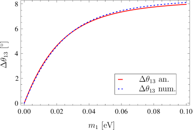
Figure 2: Change of $\theta_{13}$ in the $\mathrm{A}_{4}$ model due to the Kähler correction from the matrix $P_{\mathrm{V}}$, setting $\kappa_{\mathrm{V}}\,v^{2}/\Lambda^{2}=(0.2)^{2}$. The continuous line shows the result of equation (4.4), while the dashed line represents the result of a numerical computation.

Unlike $\theta_{13}$, which approaches $\Delta\theta_{13}\approx 8.42^{\circ}$ for $m_{1}\rightarrow\infty$, the other angles experience only minor changes under the correction $P_{\mathrm{V}}$. We see that with this correction we get close to realistic values for $\theta_{13}$ while the other angles stay almost the same.

However, we also observe opposite effects, i.e. corrections that drive the predictions of the angles away from their best fit values. For instance, the corrections due to $P_{\mathrm{IV}}$, which are independent of the neutrino masses, leave $\theta_{13}$ unchanged and change $\theta_{12}$ by $+3.2^{\circ}$ and $\theta_{23}$ by $-2.3^{\circ}$, given that we set $\kappa_{\mathrm{IV}}\,v^{2}/\Lambda^{2}=(0.2)^{2}$. We have cross–checked these analytical results by a numerical computation.

4.3 Corrections in the $\mathrm{T}^{\prime}$ model

In section 3.4 we already described the quadratic correction terms for a $\mathrm{T}^{\prime}$ model. As discussed there, due to its flavon structure the model includes all of the correction terms of the $\mathrm{A}_{4}$ model, so some of the discussion from section 4.2 still applies. However, the considered $\mathrm{T}^{\prime}$ model [19] does not predict exact tri–bi–maximal mixing so we have to consider different initial values in our analytic formulae. Moreover, a crucial assumption for the applicability of our formulae is that the model is in a basis where the charged lepton Yukawa matrix is diagonal, as stated in section 3.6.1, which is also not the case in the considered $\mathrm{T}^{\prime}$ model. Therefore, we first have to perform a basis transformation such that the charged lepton Yukawa matrix becomes diagonal. Since this is simply a basis transformation, the mixing matrix and, hence, the mixing angles are not affected. Nevertheless, the form of our correction matrices $P$ changes which we demonstrate with the help of an example. The higher–order Kähler potential term $(L\otimes{\Phi_{\nu}})^{\dagger}_{\boldsymbol{3}_{s}}(L\otimes{\Phi_{\nu}})_{\boldsymbol{3}_{a}}$, after VEV insertion, leads to the term

$$\Delta K~{}\supset~{}L^{\dagger}\,P_{\mathrm{V}}\,L+\text{h.c.}\;.$$ (4.5)

However, this is in a basis where the charged lepton Yukawa matrix is non–diagonal. The necessary basis transformation that diagonalizes it redefines the left–handed charged leptons $L$ by some matrix $V$. This leads to a modified $P$ matrix

$$L^{\dagger}\,P_{\mathrm{V}}\,L~{}\rightarrow~{}(V\,L)^{\dagger}\,P_{\mathrm{V}}\,V\,L\,~{}=~{}L^{\dagger}\,\widetilde{P}_{\mathrm{V}}\,L\;,$$ (4.6)

where we defined $\widetilde{P}_{\mathrm{V}}:=V^{\dagger}\,P_{\mathrm{V}}\,V$.

In this basis we can now use our analytic formulae on the matrix $\widetilde{P}_{\mathrm{V}}$, using the initial values for the mixing angles predicted by the original model as shown in equation (2.22), $\theta_{12}\approx 33^{\circ},\theta_{23}=45^{\circ}$ and $\theta_{13}\approx 3^{\circ}$. Furthermore, we have to consider that the model also predicts absolute neutrino masses, e.g. $m_{1}=0.0156\,\text{e\kern-0.59998ptV}$. Therefore, we cannot plot the change in mixing angles as a function of the neutrino masses, but rather against the size of the small expansion parameter $x=\mathrm{VEV}^{2}/\Lambda^{2}$ times a coefficient $\kappa_{\mathrm{V}}$ from the Kähler potential. For $\theta_{13}$ this is shown in figure 3.

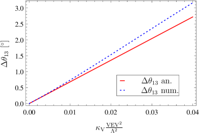
Figure 3: Change of $\theta_{13}$ in the $\mathrm{T}^{\prime}$ model due to the Kähler correction from the (modified, see text) matrix $P_{\mathrm{V}}$ up to $\kappa_{\mathrm{V}}\,\mathrm{VEV}^{2}/\Lambda^{2}=(0.2)^{2}$. The continuous line shows the result of the analytical formulae while the dashed line represents the result of a numerical computation.

In this plot we see that $\theta_{13}$ can be increased by $\Delta\theta_{13}\approx 3^{\circ}$ for $\mathrm{T}^{\prime}$, raising the value of $\theta_{13}$ up to about $6^{\circ}$ in the assumed parameter range. We also should comment that in this model two flavon triplets have the same VEV structure, as one can see in table 2.2. According to equation (2.21), both flavons $\phi$ and $\xi$ have VEVs proportional to $\left(1,1,1\right)^{T}$ and, therefore, can lead to the correction $P_{\mathrm{V}}$. In the best case, both corrections would add up and boost the maximal change to $\Delta\,\theta_{13}\approx 6^{\circ}$. This would yield $\theta_{13}\approx 9^{\circ}$ as a result, which is of the order of the experimentally measured value. However, this only applies to the very special situation in which the contributions from both flavons $\phi$ and $\xi$ add and contributions different from $P_{\mathrm{V}}$ should not spoil the result. Moreover, the VEVs in the model are generally such that $\mathrm{VEV}^{2}/\Lambda^{2}\sim\mathcal{O}(1/1000)$, in which case the Kähler corrections become negligible.

In addition to the corrections which are also present in $\mathrm{A}_{4}$, the $\mathrm{T}^{\prime}$ model has, as we showed in section 3.4, six independent corrections due to the flavon doublets $\psi$ and $\psi^{\prime}$. Let us, for example, consider the correction due to the matrix $P_{\mathsf{vi}}$ in equation (3.19b), which comes from the Kähler potential term $(L\otimes\psi^{\prime})^{\dagger}_{\boldsymbol{2^{\prime}}}(L\otimes\psi^{\prime})_{\boldsymbol{2^{\prime}}}$ as can be seen in equation (3.16). Before we can calculate the associated correction, we again have to perform a basis transformation which brings the charged lepton Yukawa matrix into diagonal form, therefore, also transforming $P_{\mathsf{vi}}\rightarrow\widetilde{P}_{\mathsf{vi}}$. Using this matrix, the initial values from equation (2.22) and the computed neutrino masses, we can again plot the changes of the mixing angles against $x=\mathrm{VEV}^{2}/\Lambda^{2}$ times a coefficient $\kappa_{\mathsf{vi}}$. As an example, we show the result for $\theta_{23}$ in figure 4.

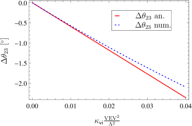
Figure 4: Change of $\theta_{23}$ in the $\mathrm{T}^{\prime}$ model due to the Kähler correction from the (modified, see text) matrix $P_{\mathsf{vi}}$ up to $\kappa_{\mathsf{vi}}\,\mathrm{VEV}^{2}/\Lambda^{2}=(0.2)^{2}$. The continuous line shows the result of the analytical formulae while the dashed line represents the result of a numerical computation.

We hence see that the Kähler corrections in the $\mathrm{T}^{\prime}$ model are less prominent than in the $\mathrm{A}_{4}$ case. Our analytical treatment as well as the Mathematica package (cf. section 3.7) allow one to determine the impact of these corrections in other concrete models with very little effort.

4.4 Further implications

4.4.1 VEV alignment

As is well known, the VEVs of fields tend to settle at symmetry enhanced points. However, since, as we have discussed in detail above, the full Lagrangean of many flavor models does not really exhibit residual symmetries, one might expect corrections also to the (holomorphic) flavon VEVs. In particular, the Kähler corrections might play a role when discussing VEV alignment, i.e. the question why the VEVs of the flavons take a particular form. In what follows, we make the simplifying assumption that the flavor sector is independent of the usual ‘hidden sector’ which is responsible for supersymmetry breakdown. Specifically, we assume that the $F$–term VEVs of the flavons are negligible.

Consider a model where the supersymmetric Lagrangean can be written in the form

$$\mathscr{L}~{}=~{}\left[K(\Psi,\Psi^{\dagger}\,\exp{(-2\,\mathsf{t}_{A}\,V_{A})})\right]_{D}+\left[\frac{1}{4}\,f_{AB}(\Psi)\,\mathcal{W}^{A}\,\mathcal{W}^{B}+\mathscr{W}(\Psi)+\text{h.c.}\right]_{F}\;,$$ (4.7)

where $\Psi$ stands for all chiral superfields of the model, $V_{A}$ are the vector superfields containing the gauge bosons, and $\mathcal{W}^{A}$ are the corresponding field strength superfields. Then, the scalar potential, whose minima determine the VEV structure, reads

$$\mathscr{V}(\psi,\psi^{*}) = \left[\frac{\partial^{2}K}{\partial(\Psi^{f})^{\dagger}\,\partial\Psi^{g}}(\psi,\psi^{*})\right]^{-1}\cdot\frac{\partial\mathscr{W}^{*}}{\partial(\Psi^{f})^{\dagger}}(\psi^{*})\cdot\frac{\partial\mathscr{W}}{\partial\Psi^{g}}(\psi)$$ (4.8)

$${}+\frac{1}{2}\left[\operatorname{Re}{\left(f_{AB}(\psi)\right)}\right]^{-1}\cdot\operatorname{Re}{\left(\frac{\partial K}{\partial\Psi^{f}}(\psi,\psi^{*})\cdot(\mathsf{t}_{A}\,\psi)^{f}\right)}$$

$${}\hphantom{{}+\frac{1}{2}\left[\operatorname{Re}{\left(f_{AB}(\psi)\right)}\right]^{-1}}\cdot\operatorname{Re}{\left(\frac{\partial K}{\partial\Psi^{g}}(\psi,\psi^{*})\cdot(\mathsf{t}_{B}\,\psi)^{g}\right)}\;,$$

where $\psi$ and $\psi^{*}$ are the scalar components of $\Psi$ and $\Psi^{\dagger}$, respectively. Before taking into account the corrections to the Kähler potential, the Kähler metric is, by assumption, diagonal,

$$\frac{\partial^{2}K}{\partial(\Psi^{f})^{\dagger}\,\partial\Psi^{g}}(\psi,\psi^{*})~{}=~{}\delta_{fg}\;,$$ (4.9)

from which it follows that the scalar potential simplifies to

$$\mathscr{V}(\psi,\psi^{*})~{}=~{}\sum_{f}\left|\frac{\partial\mathscr{W}}{\partial\Psi^{f}}(\psi)\right|^{2}+\frac{1}{2}\left[\operatorname{Re}{\left(f_{AB}(\psi)\right)}\right]^{-1}\cdot\left(\psi^{*}\,\mathsf{t}_{A}\,\psi\right)\cdot\left(\psi^{*}\,\mathsf{t}_{B}\,\psi\right)\;.$$ (4.10)

Suppose that this scalar potential has a global supersymmetric minimum at $\psi=\psi_{0}$. If $\psi$ does not break supersymmetry, $\psi_{0}$ satisfies the $F$–flatness and $D$–flatness conditions.

Let us first discuss the $F$–flatness conditions. Since the Kähler metric is invertible, the conditions

$$\frac{\partial\mathscr{W}}{\partial\Psi^{f}}(\psi_{0})~{}=~{}0,\quad\forall\,f$$ (4.11)

for the case of a canonical Kähler potential are equivalent to the conditions arising from equation (4.8), i.e. for the case of an arbitrary Kähler potential. This implies that Kähler corrections do not change the VEV alignment via the $F$–terms.

The $D$–flatness conditions require some more care. Let us first discuss the simplest and most common class of models, to which also the $\mathrm{A}_{4}$ model belongs. In these models, there is only the SM gauge symmetry, under which the flavons, however, are not charged. Hence, the flavons do not enter the $D$–flatness conditions irrespective of the Kähler potential. This, together with the invariance of the $F$–flatness conditions, implies that the vacuum alignment is completely untouched by the Kähler corrections in these models.

Let us now comment on more complicated cases. If one allows for additional gauge symmetries such as a GUT symmetry, and also for flavons having gauge charges, one, in principle, has to check case by case whether the VEV alignment is changed due to modified $D$–flatness conditions. There is, however, a simple case for which one can find a general argument. Let us assume that the additional gauge symmetry is broken by the VEVs of one or several chiral superfields $S^{f}$ which furnish irreducible representations of the gauge group, whereas all other fields, summarized in $\Psi$ in the following, are either not charged under the additional gauge symmetry or do not obtain a VEV. If one can furthermore assume that the Kähler potential factorizes as

$$K\left(\Psi,\Psi^{\dagger},S^{f},(S^{f})^{\dagger}\right)~{}=~{}K_{S}\left((S^{f})^{\dagger}\,\delta_{fg}\,S^{g}\right)\cdot K_{\Psi}\left(\Psi,\Psi^{\dagger}\right)\;,$$ (4.12)

where both $K_{S}$ and $K_{\Psi}$ should contain a constant term, the $D$–flatness conditions are equivalent to the $D$–flatness conditions of a canonical Kähler potential. In combination with the invariance of the $F$–flatness conditions this shows that the vacuum alignment stays completely unmodified by the Kähler corrections. In particular, this is fulfilled if the gauge symmetry is only broken by the VEV of one field, i.e. if there is only one field that is both charged under the gauge symmetry and attains a VEV. This applies, for example, to the $\mathrm{T}^{\prime}$ model.

In summary, we see that in most situations Kähler corrections will not interfere with the usual mechanisms for VEV alignment. This, in a way, justifies to assume that the flavons attain some ‘very symmetric’ VEVs, as for instance in the sample models discussed above.

4.4.2 Constraints from FCNCs

In supersymmetric model building, an important question concerns the flavor structure of the soft supersymmetry breaking masses and the $A$–terms. They originate from higher–dimensional terms in the superpotential and the Kähler potential. Specifically, they are induced by interactions of the matter fields with the spurion superfield $X$ that breaks supersymmetry, i.e. $X\rightarrow\theta^{2}\langle F_{X}\rangle\neq 0$.

The terms relevant for our discussion are [29]

$$\mathscr{W} \supset (Y_{e})_{fg}\,L^{f}\,R^{g}\,H_{d}-\frac{1}{\Lambda_{\mathrm{soft}}}\,(Y_{e}^{X})_{fg}\,X\,L^{f}\,R^{g}\,H_{d}\;,$$ (4.13a)

$$K \supset (L^{f})^{\dagger}\,(\mathscr{K}_{L})_{fg}\,L^{g}+\frac{1}{\Lambda_{\mathrm{soft}}}\,\left(X\,(L^{f})^{\dagger}\,(n_{L})_{fg}\,L^{g}+\text{h.c.}\right)$$ (4.13b)

$$\qquad-~{}\frac{1}{\Lambda_{\mathrm{soft}}^{2}}\,X^{\dagger}X\,(L^{f})^{\dagger}\,(k_{L})_{fg}\,L^{g}+~{}L\rightarrow R\;,$$

where $\Lambda_{\mathrm{soft}}$ represents some messenger scale, such as the Planck scale in the case of gravity mediation. The coupling matrices $Y_{e}$, $Y^{X}_{e}$, $\mathscr{K}_{L/R}$, $n_{L/R}$ and $k_{L/R}$ are functions of the flavon superfields and the cut–off scale $\Lambda$. All these matrices can obtain off–diagonal entries through non–trivial flavon contractions after the flavons acquire their VEVs. However, $\mathscr{K}_{L/R}$ and $k_{L/R}$ are Hermitean and we choose to work in a basis where $Y_{e}$ is diagonal.

The supersymmetry breaking soft masses and $A$–terms can be written as

$$\mathscr{L}_{\mathrm{soft}}~{}\supset~{}-(\widetilde{\ell}^{f})^{\dagger}\,(\widetilde{m}^{2}_{\mathrm{LL}})_{fg}\,\widetilde{\ell}^{g}-(\widetilde{r}^{f})^{\dagger}\,(\widetilde{m}^{2}_{\mathrm{RR}})_{fg}\,\widetilde{r}^{g}-\left(\widetilde{\ell}^{f}\,(A_{\mathrm{LR}})_{fg}\,\widetilde{r}^{g}+\text{h.c.}\right)\;,$$ (4.14)

where $\widetilde{\ell}$ and $\widetilde{r}$ denote the left– and right–handed slepton fields, respectively. The relations between the parameters in equation (4.13) and equation (4.14) can be obtained by replacing the spurion by its VEV and integrating out the auxiliary fields of the matter superfields. Defining $\widetilde{M}^{2}=\frac{\left|\langle F_{X}\rangle\right|^{2}}{\Lambda_{\mathrm{soft}}^{2}}$, they are given by [29]

$$\left(\widetilde{m}^{2}_{\mathrm{LL}/\mathrm{RR}}\right)_{fg} = \widetilde{M}^{2}\,\left[(k_{L/R})_{fg}+(n_{L/R}^{\dagger})_{fi}\,(n_{L/R})_{ig}\right]\;,$$ (4.15a)

$$(A_{\mathrm{LR}})_{fg} = \sqrt{\widetilde{M}^{2}}\,\left[(Y_{e}^{X})_{fg}+(n_{L})_{fi}\,(Y_{e})_{ig}+(Y_{e})_{fi}\,(n_{R})_{ig}\right]\;.$$ (4.15b)

We now turn back to equation (4.13) and analyze the couplings. By Schur’s Lemma, the matrices $\mathscr{K}_{L/R}$, $n_{L/R}$ and $k_{L/R}$ in the Kähler potential are diagonal to first order. In fact, since the left–handed lepton doublets are contained in one irreducible representation, the corresponding matrices are all proportional to the unit matrix. To simplify the following discussion, we will make the assumption that the same is true for the right–handed leptons, i.e.

$$(\mathscr{K}_{L/R})_{fg} = \delta_{fg}\;,$$ (4.16a)

$$(n_{L/R})_{fg} = \kappa_{L/R}\,\delta_{fg}\;,$$ (4.16b)

$$(k_{L/R})_{fg} = \kappa^{\prime}_{L/R}\,\delta_{fg}\;,$$ (4.16c)

with $\kappa_{L/R}$ and $\kappa^{\prime}_{L/R}$ being order one coefficients. The restriction to generation independent coefficients does not qualitatively affect the final results.

At second order, contractions of the leptons with the flavon fields are possible. When the flavons obtain their VEVs, the effective coupling matrices read

$$(\mathscr{K}_{L/R})_{fg} = \delta_{fg}-2\,x\,(P_{\mathrm{kin},L/R})_{fg}\;,$$ (4.17a)

$$(n_{L/R})_{fg} = \kappa_{L/R}\,\left[\delta_{fg}-2\,x\,(N_{L/R})_{fg}\right]\;,$$ (4.17b)

$$(k_{L/R})_{fg} = \kappa^{\prime}_{L/R}\,\left[\delta_{fg}-2\,x\,(P_{\mathrm{soft},L/R})_{fg}\right]\;,$$ (4.17c)

where $P_{\mathrm{kin},L/R}$ and $P_{\mathrm{soft},L/R}$ are Hermitean, $N_{L/R}$ arbitrary complex matrices, and $x$ is at most of the order of flavon VEV over the cut–off scale. In fact, most often $x$ is of the order $(\text{VEV}/\Lambda)^{2}$ by the arguments already outlined in section 3.1. We would like to emphasize that the matrices $P_{\mathrm{kin},L/R}$, $P_{\mathrm{soft},L/R}$ and $N_{L/R}$, which come from contractions of the lepton fields with the flavons, are a priori unrelated.

Since the Kähler metric now contains off–diagonal terms, one has to canonically normalize the lepton fields by the transformations

$$L^{f} \rightarrow L^{\prime f}=\left[\delta_{fg}+x\,(P_{\mathrm{kin},L})_{fg}\right]\,L^{f}\;,$$ (4.18a)

$$R^{f} \rightarrow R^{\prime f}=\left[\delta_{fg}+x\,(P_{\mathrm{kin},R})_{fg}\right]\,R^{f}\;,$$ (4.18b)

which leads to the transformed coupling matrices

$$(n^{\prime}_{L/R})_{fg} = \kappa_{L/R}\,\left[\delta_{fg}+2\,x\left((P_{\mathrm{kin},L/R})_{fg}-(N_{L/R})_{fg}\right)\right]\;,$$ (4.19a)

$$(k^{\prime}_{L/R})_{fg} = \kappa^{\prime}_{L/R}\,\left[\delta_{fg}+2\,x\left((P_{\mathrm{kin},L/R})_{fg}-(P_{\mathrm{soft},L/R})_{fg}\right)\right]$$ (4.19b)

to first order in $x$. Furthermore, one has to apply unitary transformations to the leptons that remove the off–diagonal elements from the charged lepton Yukawa matrix, in order to be able to compare the results to the experimental constraints. Since for $x=0$, i.e. without corrections due to the flavons, the Yukawa matrix is, by assumption, diagonal, one can write these transformations up to first order in $x$ as $U_{L/R}=1+\mathrm{i}\,x\,H_{L/R}$ with $H_{L/R}$ being Hermitean. Hence, this redefinition of fields does not affect $n_{L/R}$ and $k_{L/R}$ at linear order in $x$.

Hence, the soft masses for the sleptons in linear order in $x$ are

$$(\widetilde{m}^{2}_{\mathrm{LL}/\mathrm{RR}})_{fg} = \widetilde{M}^{2}\,\left\{\left(\kappa^{\prime}_{L/R}+\left|\kappa_{L/R}\right|^{2}\right)\,\delta_{fg}\right.$$ (4.20)

$$\quad+~{}2\,x\,\kappa^{\prime}_{L/R}\,\left[(P_{\mathrm{kin},L/R})_{fg}-(P_{\mathrm{soft},L/R})_{fg}\right]$$

$$\quad\left.+~{}2\,x\,\left|\kappa_{L/R}\right|^{2}\,\left[(P_{\mathrm{kin},L/R})_{fg}-(N_{L/R})_{fg}+\text{h.c.}\right]\right\}\;.$$

The crucial point is that all off–diagonal terms are suppressed compared to the diagonal terms by one factor of $x$. In special cases in which there are relations between $P_{\mathrm{kin},L/R}$, $P_{\mathrm{soft},L/R}$ and $N_{L/R}$, the off–diagonal terms might even vanish (almost) completely.

Before confronting this with the experimental constraints, let us first also discuss the $A$–terms without dwelling on the details. Since after all basis changes the Yukawa matrix $Y_{e}$ is diagonal, the off–diagonal elements of the second and third term of $A_{LR}$ in equation (4.15b) are suppressed by one factor of $x$. Moreover, they are suppressed by the smallness of the lepton masses.

The coupling matrix $Y_{e}^{X}$ in equation (4.13) can only arise from the same flavon contractions as the Yukawa matrix $Y_{e}$. Neglecting the possibility of fine–tuning, our assumption of a diagonal Yukawa thus implies diagonal $Y_{e}^{X}$. Although the precise size of the entries of $Y_{e}^{X}$ may differ from the lepton masses, one should assume that they are of the same order of magnitude. Since $Y_{e}^{X}$ does not have to be proportional to $Y_{e}$, the effects of the transformation (4.18) on $Y_{e}^{X}$ are not completely undone by the unitary rotation to the charged lepton mass basis. However, all off–diagonal terms are at most of the order $x$ and, furthermore, suppressed by the smallness of the diagonal entries.

Let us now discuss the experimental constraints. We showed above that the Kähler corrections induce off–diagonal terms for the soft masses and the $A$–terms. Therefore, FCNCs are induced, in general by slepton, chargino, higgsino and neutralino loops. The strongest constraints are given by the decay $\mu\rightarrow e\,\gamma$. The SUSY contribution to this process through photino and slepton loops is given by [30]

$$\mathrm{Br}(\mu\rightarrow e\,\gamma) = \frac{12\,\pi\,\alpha^{3}}{G_{\mathrm{F}}^{2}\,m_{\mathrm{SUSY}}^{4}}\left|(\delta_{12})_{\mathrm{LL}}\,M_{3}(y)+\frac{\sqrt{y}\,m_{\mathrm{SUSY}}}{m_{\mu}}(\delta_{12})_{\mathrm{LR}}\,M_{1}(y)\right|^{2}$$ (4.21)

$$\vphantom{\frac{12\,\pi\,\alpha^{3}}{G_{\mathrm{F}}^{2}\,m_{\mathrm{SUSY}}^{4}}}\quad+~{}\left(\mathrm{L}\leftrightarrow\mathrm{R}\right)\;,$$

where $M_{1}(y)$ and $M_{3}(y)$ are loop factors depending on the mass–squared ratio between photino and slepton, $y=m_{\widetilde{\gamma}}^{2}/m_{\widetilde{\ell}}^{2}$, where we set $m_{\widetilde{\ell}}\approx m_{\mathrm{SUSY}}$. Their precise expressions can be found in [30]. For our purposes it is enough to state that the functions $M_{3}$ and $M_{1}$ are bounded by $M_{3}(y)<0.083$ and $M_{1}(y)<0.5$. More importantly, $(\delta_{12})_{\mathrm{LL}}$ and $(\delta_{12})_{\mathrm{LR}}$ are the mass insertion parameters, i.e. the ratio between the off–diagonal and the diagonal elements of the soft masses or the $A$–terms, respectively. Through equation (4.20) we can estimate $(\delta_{12})_{\mathrm{LL}}$ to be of the order of $x$. The chirality changing mass insertion $(\delta_{12})_{\mathrm{LR}}$ is determined by the $A$–term, which again is proportional to $x$. Furthermore, one might expect, as argued above, that the $A$–term is proportional to a parameter of the order of the corresponding Yukawa coupling. Therefore, we can estimate the $A$–term to be of the order $\widetilde{M}\,x\,y_{\mu}$ , which yields $(\delta_{12})_{\mathrm{LR}}~{}\simeq~{}(x\,m_{\mu})/m_{\mathrm{SUSY}}$ for the mass insertion parameter in (4.21).

In the previous sections we assumed the expansion parameter $x$ to be maximally of the order Cabibbo angle squared, i.e. $x\lesssim 0.04$. Using this value in our mass insertion parameters we can give a lower bound for the slepton mass $m_{\mathrm{SUSY}}$ in order to satisfy the current experimental limit of $\mathrm{Br}(\mu\rightarrow e\,\gamma)_{\mathrm{exp}}<2.4\times 10^{-12}$ [27]. For a photino to slepton mass–squared ratio of $y=5$, we have $m_{\mathrm{SUSY}}\geq 700\>\text{Ge\kern-0.59998ptV}$, for $y=2$, we get $m_{\mathrm{SUSY}}\geq 1\>\text{Te\kern-0.59998ptV}$, and for $y=0.5$, we have $m_{\mathrm{SUSY}}\geq 1.2\>\text{Te\kern-0.59998ptV}$. Furthermore, for $m_{\mathrm{SUSY}}\geq 1.4\>\text{Te\kern-0.59998ptV}$, the experimental limits are always satisfied, independent of the photino to slepton mass–squared ratio. This shows that constraints from FCNCs do not rule out sizable Kähler corrections for reasonable values of the soft SUSY breaking mass scale.

5 Conclusions

We have discussed the impact of Kähler corrections on the predictions of models with spontaneously broken flavor symmetries. We find that these corrections are, in general, sizable since they are controlled by the ratio of flavon VEV over the fundamental scale, which also sets the scale of the expansion parameter for the entries of the coupling and mass matrices. Furthermore, it appears hard to avoid Kähler corrections because the corresponding terms cannot be forbidden by means of conventional symmetries. In addition, the coefficients of such terms entail new parameters, which reduce the predictivity of the respective models. In view of these results, it appears to be premature to ‘rule out’ certain symmetry groups by looking at the holomorphic terms only, as has been done recently in various scans [31, 32].

Let us stress at this point that the situation in non–supersymmetric settings is similar. In the non–supersymmetric case, it is, of course, also possible to write down higher–order corrections to the kinetic terms which are induced by the flavon VEVs. As it turns out these induce changes of the mixing parameters identical to the supersymmetric case, therefore, extending the applicability of our discussion to non–supersymmetric models.

In particular, we have presented a full derivation of analytic formulae which describe the change of the mixing parameters. We have applied these formulae to two example models, one based on the flavor symmetry $G_{\mathrm{F}}=\mathrm{A}_{4}\times\mathbbm{Z}_{4}$ [18] and one based on $G_{\mathrm{F}}=\mathrm{T}^{\prime}\times\mathbbm{Z}_{12}\times\mathbbm{Z}_{12}$ [19]. We have demonstrated that, for the simple $\mathrm{A}_{4}$ model which predicts tri–bi–maximal mixing at the leading order, one of the flavon VEVs induces a large $\theta_{13}$ value that is compatible with current experimental limits [21, 22, 23]. On the other hand, the VEV pattern in the $\mathrm{T}^{\prime}$ model is such that Kähler corrections are not too large unless the Kähler coefficients are large. This can easily be understood with the aid of the analytic formulae derived in this paper, and can also be checked with the associated Mathematica package.

Furthermore, we have shown that the Kähler corrections do not pose a threat to the VEV alignment. Moreover, we have argued that they also do not induce significant flavor changing neutral currents, i.e.  for reasonably large soft masses, the size of the flavor violating terms is well within the current experimental bounds. Hence, also the vanishing of FCNCs cannot be used to constrain the Kähler corrections considerably.

In conclusion, we argue that, in the supersymmetric context, a theory of flavor requires a better understanding of the Kähler potential. Such an understanding may be obtained in higher–dimensional settings, where effective couplings can be computed from wave–function overlaps (cf. e.g. [33, 34]), and non–Abelian discrete symmetries may be related to the geometry of compact space (cf. e.g. [35]). In this regard, it appears also promising to derive flavor models from string theory, where the non–Abelian discrete symmetries have a clear geometrical interpretation [36, 37, 38]. In certain settings, the Kähler potentials are known to some extent [39]; some information can be inferred from the transformation behavior of the fields under the modular group [40, 41]; however, closed expressions for higher–order terms have not yet been worked out.

Acknowledgments

We would like to thank C. Albright and J. Heckman for useful discussions. M.-C.C. would like to thank TU München, where part of the work was done, for hospitality. M.R. would like to thank the UC Irvine, where part of this work was done, for hospitality. This work was partially supported by the Deutsche Forschungsgemeinschaft (DFG) through the cluster of excellence “Origin and Structure of the Universe” and the Graduiertenkolleg “Particle Physics at the Energy Frontier of New Phenomena”. This research was done in the context of the ERC Advanced Grant project “FLAVOUR” (267104), and was partially supported by the U.S. National Science Foundation under Grant No. PHY-0970173. We thank the Aspen Center for Physics, where this discussion was initiated, the Galileo Galilei Institute for Theoretical Physics (GGI), the Simons Center for Geometry and Physics in Stony Brook, and the Center for Theoretical Underground Physics and Related Areas (CETUP* 2012) in South Dakota for their hospitality and for partial support during the completion of this work.

Appendix A Conventions

A.1 Parametrization of $U_{\mathrm{PMNS}}$

The parametrization of the PMNS–matrix used in this text is shown here. First, $U_{\mathrm{PMNS}}$ is decomposed in the product of a diagonal phase matrix containing the unphysical lepton phases, a CKM–like matrix $V$ and a diagonal matrix containing the two Majorana phases,

$$U_{\mathrm{PMNS}}~{}=~{}\operatorname{diag}{(\mathrm{e}^{\mathrm{i}\delta_{e}},\,\mathrm{e}^{\mathrm{i}\delta_{\mu}},\,\mathrm{e}^{\mathrm{i}\delta_{\tau}})}\cdot V(\theta_{12},\,\theta_{13},\,\theta_{13},\,\delta)\cdot\operatorname{diag}{(\mathrm{e}^{-\mathrm{i}\phi_{1}/2},\,\mathrm{e}^{\mathrm{i}\phi_{2}/2},\,1)}\;.$$ (A.1)

The matrix $V$ itself is parametrized as

$$V~{}=~{}\begin{pmatrix}c_{12}\,c_{13}&s_{12}\,c_{13}&s_{13}\,\mathrm{e}^{-\mathrm{i}\delta}\\ -s_{12}\,c_{23}-c_{12}\,s_{23}\,s_{13}\,\mathrm{e}^{\mathrm{i}\delta}&c_{12}\,c_{23}-s_{12}\,s_{23}\,s_{13}\,\mathrm{e}^{\mathrm{i}\delta}&s_{23}\,c_{13}\\ s_{12}\,s_{23}-c_{12}\,c_{23}\,s_{13}\,\mathrm{e}^{\mathrm{i}\delta}&-c_{12}\,s_{23}-s_{12}\,c_{23}\,s_{13}\,\mathrm{e}^{\mathrm{i}\delta}&c_{23}\,c_{13}\end{pmatrix}\;.$$ (A.2)

Here, $s_{ij}$ denotes $\sin\theta_{ij}$ and $c_{ij}$ denotes $\cos\theta_{ij}$.

A.2 $\mathrm{A}_{4}$

In section 3 we provided possible Kähler corrections for models based on the non–Abelian flavor group $\mathrm{A}_{4}$. In this appendix, we recall the most important aspects of the $\mathrm{A}_{4}$ group, which is the symmetry group of the regular tetrahedron. It has four inequivalent irreducible representations, including three singlets $\boldsymbol{1}\,,\boldsymbol{1}^{\prime}\,,\boldsymbol{1}^{\prime\prime}$ and one triplet $\boldsymbol{3}$. Throughout the literature there are mainly two different bases that have been used for $\mathrm{A}_{4}$. In section 3 we utilize the basis in which the generators $S$ and $T$ are represented as

$$S=\frac{1}{3}\left(\begin{array}[]{ccc}-1&2&2\\ 2&-1&2\\ 2&2&-1\end{array}\right)\;,\qquad T=\left(\begin{array}[]{ccc}1&0&0\\ 0&\omega^{2}&0\\ 0&0&\omega\end{array}\right)\;,\qquad\mathrm{with}\qquad\omega=\mathrm{e}^{\frac{2\pi\mathrm{i}}{3}}\;.$$ (A.3)

These generators give us the multiplication rule

$$\boldsymbol{3}\otimes\boldsymbol{3}~{}=~{}\boldsymbol{1}\oplus\boldsymbol{1^{\prime}}\oplus\boldsymbol{1^{\prime\prime}}\oplus\boldsymbol{3}_{\mathrm{s}}\oplus\boldsymbol{3}_{\mathrm{a}}\;,$$ (A.4)

where $\boldsymbol{3}_{\mathrm{s}}$ and $\boldsymbol{3}_{\mathrm{a}}$ denote the symmetric and the antisymmetric triplet combinations, respectively. In terms of the components of the two triplets, $\boldsymbol{a}$ and $\boldsymbol{b}$,

$$\left(\boldsymbol{a}\otimes\boldsymbol{b}\right)_{\boldsymbol{1}} = a_{1}\,b_{1}+a_{2}\,b_{3}+a_{3}\,b_{2}\;,$$ (A.5a)

$$\left(\boldsymbol{a}\otimes\boldsymbol{b}\right)_{\boldsymbol{1^{\prime}}} = a_{2}\,b_{2}+a_{1}\,b_{3}+a_{3}\,b_{1}\;,$$ (A.5b)

$$\left(\boldsymbol{a}\otimes\boldsymbol{b}\right)_{\boldsymbol{1^{\prime\prime}}} = a_{3}\,b_{3}+a_{1}\,b_{2}+a_{2}\,b_{1}\;,$$ (A.5c)

$$\left(\boldsymbol{a}\otimes\boldsymbol{b}\right)_{\boldsymbol{3}_{\mathrm{s}}} = \frac{1}{\sqrt{2}}\,\left(\begin{array}[]{c}2a_{1}\,b_{1}-a_{2}\,b_{3}-a_{3}\,b_{2}\\ 2a_{3}\,b_{3}-a_{1}\,b_{2}-a_{2}\,b_{1}\\ 2a_{2}\,b_{2}-a_{1}\,b_{3}-a_{3}\,b_{1}\end{array}\right)\;,$$ (A.5g)

$$\left(\boldsymbol{a}\otimes\boldsymbol{b}\right)_{\boldsymbol{3}_{\mathrm{a}}} = \mathrm{i}\,\sqrt{\frac{3}{2}}\,\left(\begin{array}[]{c}a_{2}\,b_{3}-a_{3}\,b_{2}\\ a_{1}\,b_{2}-a_{2}\,b_{1}\\ a_{3}\,b_{1}-a_{1}\,b_{3}\end{array}\right)\;,$$ (A.5k)

where $\left(\boldsymbol{a}\otimes\boldsymbol{b}\right)_{\boldsymbol{R}}$ indicates that $\boldsymbol{a}$ and $\boldsymbol{b}$ are contracted to the representation $\boldsymbol{R}$. Note that there are different conventions for normalizing the triplets $\boldsymbol{3}_{i}$ in the literature, and the corresponding factors can be absorbed in the Kähler coefficients.

In another basis, $\mathrm{A}_{4}$ is generated by

$$\widetilde{S}~{}=~{}\left(\begin{array}[]{ccc}1&0&0\\ 0&-1&0\\ 0&0&-1\end{array}\right)\;,\qquad\widetilde{T}~{}=~{}\left(\begin{array}[]{ccc}0&0&1\\ 1&0&0\\ 0&1&0\end{array}\right)\;,$$ (A.6)

which is related to our basis through the unitary transformation matrix

$$U_{\omega}~{}=~{}\frac{1}{\sqrt{3}}\left(\begin{array}[]{ccc}1&1&1\\ 1&\omega&\omega^{2}\\ 1&\omega^{2}&\omega\end{array}\right)\;.$$ (A.7)

The relation between the two bases is then given by $\widetilde{S}=U_{\omega}\,S\,U_{\omega}^{\dagger}$ and $\widetilde{T}=U_{\omega}\,T\,U_{\omega}^{\dagger}$.

It is important to note that this basis transformation also relates the different flavon VEVs to one another. This means that the VEV $(v,v,v)^{T}$ in one basis is equivalent to the VEV $(v^{\prime},0,0)^{T}$ in the other basis, and vice versa.

Appendix B Examples for analytic formulae

We present examples of the analytic formulae for corrections due to $P_{L}$ in

$$K~{}=~{}L^{\dagger}\,(1+x_{L}\,P_{L})\,L+R^{\dagger}\,R\;,$$ (B.1)

where $P_{L}$ is replaced by one of the nine basis matrices $P_{i}$, as shown in equation (3.20). We take the tri–bi–maximal mixing as initial condition for the mixing parameters, i.e.

$$\theta_{12} = \arcsin{\frac{1}{\sqrt{3}}}\;,\quad\theta_{13}~{}=~{}0,\quad\theta_{23}~{}=~{}\frac{\pi}{4}\;,\quad\delta~{}=~{}\text{undefined}\;,$$

$$\delta_{e} = \pi\;,\quad\delta_{\mu}~{}=~{}\pi\;,\quad\delta_{\tau}~{}=~{}0\;,\quad\varphi_{1}~{}=~{}\varphi_{2}~{}=~{}2\pi\;.$$ (B.2)

The CP phase $\delta$ is determined from the formulae by demanding that the change of $\delta$ is analytical at $\theta_{13}=0$ for each of the $P_{i}$, which yields $\delta=0$ for $i=1,\dots,6$ and $\delta=-\pi/2$ for $i=7,8,9$. The neutrino masses $m_{i}$ are left unspecified. The pronounced hierarchy of the charged lepton masses, i.e. $m_{\tau}\gg m_{\mu}\gg m_{e}$, is used to simplify the results. In leading order in an expansion in the small mass ratios, the charged lepton masses completely drop out from the formulae. We obtain the following analytical expressions for the changes of the mixing angles:

• For $P=P_{1}$:

  $$\Delta\theta_{12}^{(1)} = x_{L}\,\frac{1}{3\,\sqrt{2}}\,\frac{m_{1}+m_{2}}{m_{1}-m_{2}}\;,$$ (B.3a)

  $$\Delta\theta_{13}^{(1)} = 0\;,$$ (B.3b)

  $$\Delta\theta_{23}^{(1)} = 0\;.$$ (B.3c)

• For $P=P_{2}$:

  $$\Delta\theta_{12}^{(2)} = x_{L}\,\frac{1}{3\,\sqrt{2}}\,\frac{2\,m_{1}-m_{2}}{m_{1}-m_{2}}\;,$$ (B.4a)

  $$\Delta\theta_{13}^{(2)} = x_{L}\,\frac{1}{3\,\sqrt{2}}\,\frac{3\,m_{1}\,m_{2}-2\,m_{1}\,m_{3}-m_{2}\,m_{3}}{(m_{1}-m_{3})\,(m_{2}-m_{3})}\;,$$ (B.4b)

  $$\Delta\theta_{23}^{(2)} = x_{L}\,\frac{1}{3}\,\frac{m_{3}\,(m_{1}-m_{2})}{(m_{1}-m_{2})\,(m_{2}-m_{3})}\;.$$ (B.4c)

• For $P=P_{3}$:

  $$\Delta\theta_{12}^{(3)} = -x_{L}\,\frac{1}{6\,\sqrt{2}}\,\frac{m_{1}+m_{2}}{m_{1}-m_{2}}\;,$$ (B.5a)

  $$\Delta\theta_{13}^{(3)} = x_{L}\,\frac{1}{3\,\sqrt{2}}\,\frac{m_{3}\,(m_{1}-m_{2})}{(m_{1}-m_{3})\,(m_{2}-m_{3})}\;,$$ (B.5b)

  $$\Delta\theta_{23}^{(3)} = x_{L}\,\frac{1}{12}\,\frac{m_{1}\,(3\,m_{2}+m_{3})-m_{3}\,(m_{2}+3\,m_{3})}{(m_{1}-m_{3})\,(m_{2}-m_{3})}\;.$$ (B.5c)

• For $P=P_{4}$:

  $$\Delta\theta_{12}^{(4)} = x_{L}\,\frac{1}{3\,\sqrt{2}}\,\frac{2\,m_{1}-m_{2}}{m_{1}-m_{2}}\;,$$ (B.6a)

  $$\Delta\theta_{13}^{(4)} = -x_{L}\,\frac{1}{3\,\sqrt{2}}\,\frac{3\,m_{1}\,m_{2}-2\,m_{1}\,m_{3}-m_{2}\,m_{3}}{(m_{1}-m_{3})\,(m_{2}-m_{3})}\;,$$ (B.6b)

  $$\Delta\theta_{23}^{(4)} = -x_{L}\,\frac{1}{3}\,\frac{m_{3}\,(m_{1}-m_{2})}{(m_{1}-m_{3})\,(m_{2}-m_{3})}\;.$$ (B.6c)

• For $P=P_{5}$:

  $$\Delta\theta_{12}^{(5)} = -x_{L}\,\frac{1}{3\,\sqrt{2}}\,\frac{m_{1}+m_{2}}{m_{1}-m_{2}}\;,$$ (B.7a)

  $$\Delta\theta_{13}^{(5)} = 0\;,$$ (B.7b)

  $$\Delta\theta_{23}^{(5)} = -x_{L}\,\frac{1}{2}\;.$$ (B.7c)

• For $P=P_{6}$:

  $$\Delta\theta_{12}^{(6)} = -x_{L}\,\frac{1}{6\,\sqrt{2}}\,\frac{m_{1}+m_{2}}{m_{1}-m_{2}}\;,$$ (B.8a)

  $$\Delta\theta_{13}^{(6)} = -x_{L}\,\frac{1}{3\,\sqrt{2}}\,\frac{m_{3}\,(m_{1}-m_{2})}{(m_{1}-m_{3})\,(m_{2}-m_{3})}\;,$$ (B.8b)

  $$\Delta\theta_{23}^{(6)} = x_{L}\,\frac{1}{12}\,\frac{m_{1}\,(3\,m_{2}+m_{3})-m_{3}\,(m_{2}+3\,m_{3})}{(m_{1}-m_{3})\,(m_{3}-m_{2})}\;.$$ (B.8c)

• For $P=P_{7}$:

  $$\Delta\theta_{12}^{(7)} = 0\;,$$ (B.9a)

  $$\Delta\theta_{13}^{(7)} = -x_{L}\,\frac{1}{3\,\sqrt{2}}\,\frac{3\,m_{1}\,m_{2}+2\,m_{1}\,m_{3}+m_{2}\,m_{3}}{(m_{1}+m_{3})\,(m_{2}+m_{3})}\;,$$ (B.9b)

  $$\Delta\theta_{23}^{(7)} = 0\;.$$ (B.9c)

• For $P=P_{8}$:

  $$\Delta\theta_{12}^{(8)} = 0\;,$$ (B.10a)

  $$\Delta\theta_{13}^{(8)} = x_{L}\,\frac{1}{3\,\sqrt{2}}\,\frac{3\,m_{1}\,m_{2}+2\,m_{1}\,m_{3}+m_{2}\,m_{3}}{(m_{1}+m_{3})\,(m_{2}+m_{3})}\;,$$ (B.10b)

  $$\Delta\theta_{23}^{(8)} = 0\;.$$ (B.10c)

• For $P=P_{9}$:

  $$\Delta\theta_{12}^{(9)} = 0\;,$$ (B.11a)

  $$\Delta\theta_{13}^{(9)} = -x_{L}\,\frac{\sqrt{2}}{3}\,\frac{m_{3}\,(m_{1}-m_{2})}{(m_{1}+m_{3})\,(m_{2}+m_{3})}\;,$$ (B.11b)

  $$\Delta\theta_{23}^{(9)} = 0\;.$$ (B.11c)

As discussed in the main text, a general $P$ matrix can be decomposed into the nine basis matrices $P_{i}$,

$$P~{}=~{}\sum\limits_{i=1}^{9}x_{L}^{(i)}\,P_{i}\;,$$ (B.12)

and the resulting changes for the mixing angles are then given by

$$\Delta\theta_{jk}~{}=~{}\sum\limits_{i=1}^{9}x_{L}^{(i)}\,\Delta\theta_{jk}^{(i)}\;.$$ (B.13)

With our Mathematica package (cf. section 3.7) one can derive similar expressions for other initial conditions on the mixing parameters.

References

- [1] G. Altarelli and F. Feruglio, Rev.Mod.Phys. 82 (2010), 2701, arXiv:1002.0211 [hep-ph].
- [2] S. F. King and C. Luhn, arXiv:1301.1340 [hep-ph].
- [3] F. Vissani, arXiv:hep-ph/9708483 [hep-ph].
- [4] V. D. Barger, S. Pakvasa, T. J. Weiler, and K. Whisnant, Phys.Lett. B437 (1998), 107, arXiv:hep-ph/9806387 [hep-ph].
- [5] P. Harrison, D. Perkins, and W. Scott, Phys.Lett. B530 (2002), 167, arXiv:hep-ph/0202074 [hep-ph].
- [6] E. Ma, Phys.Rev. D70 (2004), 031901, arXiv:hep-ph/0404199 [hep-ph].
- [7] M. Leurer, Y. Nir, and N. Seiberg, Nucl.Phys. B398 (1993), 319, arXiv:hep-ph/9212278 [hep-ph].
- [8] M. Leurer, Y. Nir, and N. Seiberg, Nucl. Phys. B420 (1994), 468, hep-ph/9310320.
- [9] E. Dudas, S. Pokorski, and C. A. Savoy, Phys.Lett. B356 (1995), 45, arXiv:hep-ph/9504292 [hep-ph].
- [10] S. K. Soni and H. A. Weldon, Phys.Lett. B126 (1983), 215.
- [11] S. F. King and I. N. Peddie, Phys.Lett. B586 (2004), 83, arXiv:hep-ph/0312237 [hep-ph].
- [12] J. Espinosa and A. Ibarra, JHEP 0408 (2004), 010, arXiv:hep-ph/0405095 [hep-ph].
- [13] S. Antusch, J. Kersten, M. Lindner, and M. Ratz, Nucl.Phys. B674 (2003), 401, arXiv:hep-ph/0305273 [hep-ph].
- [14] S. Antusch, J. Kersten, M. Lindner, M. Ratz, and M. A. Schmidt, JHEP 03 (2005), 024, hep-ph/0501272.
- [15] S. Antusch, S. F. King, and M. Malinsky, Phys.Lett. B671 (2009), 263, arXiv:0711.4727 [hep-ph].
- [16] S. Antusch, S. F. King, and M. Malinsky, JHEP 0805 (2008), 066, arXiv:0712.3759 [hep-ph].
- [17] M.-C. Chen, M. Fallbacher, M. Ratz, and C. Staudt, Phys.Lett. B718 (2012), 516, arXiv:1208.2947 [hep-ph].
- [18] G. Altarelli and F. Feruglio, Nucl.Phys. B741 (2006), 215, arXiv:hep-ph/0512103 [hep-ph].
- [19] M.-C. Chen and K. Mahanthappa, Phys.Lett. B681 (2009), 444, arXiv:0904.1721 [hep-ph].
- [20] G. Fogli, E. Lisi, A. Marrone, D. Montanino, A. Palazzo, et al., Phys.Rev. D86 (2012), 013012, arXiv:1205.5254 [hep-ph].
- [21] DOUBLE-CHOOZ Collaboration, Y. Abe et al., Phys.Rev.Lett. 108 (2012), 131801, arXiv:1112.6353 [hep-ex].
- [22] DAYA-BAY Collaboration, F. An et al., Phys.Rev.Lett. 108 (2012), 171803, arXiv:1203.1669 [hep-ex].
- [23] RENO collaboration, J. Ahn et al., Phys.Rev.Lett. 108 (2012), 191802, arXiv:1204.0626 [hep-ex].
- [24] G. Altarelli, F. Feruglio, and L. Merlo, arXiv:1205.5133 [hep-ph].
- [25] H. Ishimori, T. Kobayashi, H. Ohki, Y. Shimizu, H. Okada, et al., Prog.Theor.Phys.Suppl. 183 (2010), 1, arXiv:1003.3552 [hep-th].
- [26] M. Lindner, M. Ratz, and M. A. Schmidt, JHEP 09 (2005), 081, hep-ph/0506280.
- [27] Particle Data Group, J. Beringer et al., Phys.Rev. D86 (2012), 010001.
- [28] W. Grimus, L. Lavoura, and P. Ludl, J.Phys. G36 (2009), 115007, arXiv:0906.2689 [hep-ph].
- [29] S. P. Martin, hep-ph/9709356.
- [30] F. Gabbiani, E. Gabrielli, A. Masiero, and L. Silvestrini, Nucl.Phys. B477 (1996), 321, arXiv:hep-ph/9604387 [hep-ph].
- [31] K. M. Parattu and A. Wingerter, Phys.Rev. D84 (2011), 013011, arXiv:1012.2842 [hep-ph].
- [32] M. Holthausen, K. S. Lim, and M. Lindner, arXiv:1212.2411 [hep-ph].
- [33] N. Arkani-Hamed, T. Gregoire, and J. Wacker, JHEP 03 (2002), 055, hep-th/0101233.
- [34] H. M. Lee, H. P. Nilles, and M. Zucker, Nucl. Phys. B680 (2004), 177, hep-th/0309195.
- [35] G. Altarelli, F. Feruglio, and Y. Lin, Nucl.Phys. B775 (2007), 31, arXiv:hep-ph/0610165 [hep-ph].
- [36] T. Kobayashi, H. P. Nilles, F. Plöger, S. Raby, and M. Ratz, Nucl. Phys. B768 (2007), 135, hep-ph/0611020.
- [37] H. P. Nilles, M. Ratz, and P. K. Vaudrevange, arXiv:1204.2206 [hep-ph].
- [38] M. Berasaluce-Gonzalez, P. Camara, F. Marchesano, D. Regalado, and A. Uranga, JHEP 1209 (2012), 059, arXiv:1206.2383 [hep-th].
- [39] M. Cvetič, J. Louis, and B. A. Ovrut, Phys. Lett. B206 (1988), 227.
- [40] L. J. Dixon, V. Kaplunovsky, and J. Louis, Nucl. Phys. B329 (1990), 27.
- [41] L. E. Ibáñez and D. Lüst, Nucl. Phys. B382 (1992), 305, hep-th/9202046.