On Neumann and oblique derivatives boundary conditions for nonlocal elliptic equations

Abstract.

Inspired by the penalization of the domain approach of Lions & Sznitman, we give a sense to Neumann and oblique derivatives boundary value problems for nonlocal, possibly degenerate elliptic equations. Two different cases are considered: (i) homogeneous Neumann boundary conditions in convex, possibly non-smooth and unbounded domains, and (ii) general oblique derivatives boundary conditions in smooth, bounded, and possibly non-convex domains. In each case we give apropriate definitions of viscosity solutions and prove uniqueness of solutions of the corresponding boundary value problems. We prove that these boundary value problems arise in the penalization of the domain limit from whole space problems and obtain as a corollary the existence of solutions of these problems.

1. Introduction

Inspired by the penalization of the domain approach of Lions & Sznitman [20] (see also [21, 23]), we give a sense to Neumann and oblique derivatives boundary value problems for nonlocal degenerate elliptic partial integro-differential equations (PIDEs in short). Because of the nonlocal nature of our PIDEs posed in a domain $\Omega$, the boundary conditions have then to be imposed not only at the boundary $\partial\Omega$, but possibly in all of the complement $\Omega^{c}$. At least boundary conditions must be imposed in the union of the supports of the jump measures (see below).

To be more specific, we consider PIDEs of the form

$$F(x,u,Du,D^{2}u,{\mathcal{I}}[u](x))=\ 0\quad\text{in}\quad\Omega,$$ (1.1)

with extended Neumann/oblique derivatives boundary conditions

$$Du(x)\cdot\gamma(x)=\ g(x)\quad\text{in}\quad\Omega^{c}.$$ (1.2)

Here $\Omega$ is a domain in ${\mathbb{R}}^{N}$ and $F$ is a real-valued, continuous function defined on ${\mathbb{R}}^{N}\times{\mathbb{R}}\times{\mathbb{R}}^{N}\times\mathbb{S}^{N}\times{\mathbb{R}}$, where $\mathbb{S}^{N}$ is the space of $N\times N$ symmetric matrices. We assume that $F$ is degenerate elliptic which, in this nonlocal setting, means that for any $x\in{\mathbb{R}}^{N}$, $u\in{\mathbb{R}}$, $p\in{\mathbb{R}}^{N}$, $M,N\in\mathbb{S}^{N}$ and $l_{1},l_{2}\in{\mathbb{R}}$,

$$F(x,u,p,M,l_{1})\leq F(x,u,p,N,l_{2})\quad\hbox{when}\quad M\geq N,\ l_{1}\geq l_{2},$$ (1.3)

where $M\geq N$ has to be understood in the sense of the usual partial ordering on symmetric matrices. Our assumptions cover the cases of general linear (see example below) and nonlinear equations and, in particular, Bellman-Isaacs equations of control and game theory.

The equation is nonlocal because of its dependence on the nonlocal operator ${\mathcal{I}}[u]$ which we assume to be of Lévy-Ito type. For any smooth bounded function $\phi$ and for any $x\in{\mathbb{R}}^{N}$,

$${\mathcal{I}}[\phi](x)=\int_{{\mathbb{R}}^{N}}\left[\phi(x+j(x,z))-\phi(x)-D\phi(x)\cdot j(x,z)1_{B}(z)\right]\,d\mu(z),$$ (1.4)

where $B\subset{\mathbb{R}}^{N}$ is the unit ball, $1_{B}$ the indicator function of $B$, $\mu$ – the Lévy measure – is a positive Radon measure on ${\mathbb{R}}^{M}\setminus\{0\}$ and $j:{\mathbb{R}}^{N}\times{\mathbb{R}}^{M}\to{\mathbb{R}}^{N}$ is a function which is $\mu$-measurable in $z$ and continuous in $x$ for $\mu$-a.e. $z$, and there exists a constant $c(j)>0$ such that

$$\int_{{\mathbb{R}}^{N}}|z|^{2}\wedge 1\ d\mu(z)<\infty\quad\text{and}\quad|j(x,z)|\leq c(j)|z|\quad\text{for any}\;|z|<1,\ x\in{\mathbb{R}}^{N}.$$ (1.5)

A Taylor expansion shows that ${\mathcal{I}}[\phi]$ is well-defined under (1.5). We will assume that (1.5) holds throughout this paper. The operator ${\mathcal{I}}$ is the generator of a stochastic jump process which solves a stochastic differential equation involving a general jump term/Poisson random measure, cf. [14, 24]. Included are generators of all pure jump Levy processes [1] as well most Levy models arising in Finance [11].

A typical example of Equation (1.1) is the linear equation

$$a(-\Delta)^{\frac{\alpha}{2}}u-{\rm Tr}(A(x)D^{2}u)-b(x)\cdot Du+\lambda(x)u=f(x)\quad\text{in}\quad\Omega,$$ (1.6)

where $a\in{\mathbb{R}}$, $A,b,\lambda,f$ are continuous functions on $\overline{\Omega}$, taking values respectively in $\mathbb{S}^{N}$, ${\mathbb{R}}^{N}$, $(0,+\infty)$ and ${\mathbb{R}}$, and, for $\alpha\in(0,2)$, ${\mathcal{I}}=-(-\Delta)^{\frac{\alpha}{2}}$ is the Fractional Laplacian in ${\mathbb{R}}^{N}$, the generator of the symmetric $\alpha$-stable processes. It is defined e.g. by (1.4) with $j(x,z)\equiv z$ and $\displaystyle d\mu(z)=c_{\alpha}\frac{dz}{|z|^{N+\alpha}}$ for some constant $c_{\alpha}>0$. To satisfy the (degenerate) ellipticity condition (1.3), we must impose that both $a\geq 0$ and $A\geq 0$ in $\overline{\Omega}$.

It is the definition of ${\mathcal{I}}$ (cf. (1.4)) that requires $u$ to be defined in all of ${\mathbb{R}}^{N}$, and hence that the boundary condition must be posed in all of $\Omega^{c}$.

For the boundary (or exterior) condition (1.2), we assume that

• The functions $\gamma:{\mathbb{R}}^{N}\to{\mathbb{R}}^{N}$ and $g:{\mathbb{R}}^{N}\to{\mathbb{R}}$ are bounded Lipschitz continuous functions, and there exists $\nu>0$ such that $\gamma(x)\cdot n(x)\geq\nu$ for any $x\in\partial\Omega$.

• For any $x\in\overline{\Omega}^{c}$, $\tau_{x}:=\inf_{t>0}\{X_{x}(t)\in\overline{\Omega}\}<+\infty$, where $X_{x}(\cdot)$ solves

  $$X_{x}(0)=x\qquad\text{and}\qquad\dot{X}_{x}(t)=-\gamma(X_{x}(t))\quad\text{for}\quad t>0.$$ (1.7)

Assumption (BC1) is sufficient for (1.2) to really play the role of a boundary condition in the case of local equations. Assumption (BC2) states that integral curves of the vector field $-\gamma$ starting from any point $x\in\Omega^{c}$, will reach the boundary $\partial\Omega$ in finite time. This is a natural condition for a Neumann type boundary condition, and it is very closely related to the idea of the “penalization of the domain” method of Lions & Sznitman [20] (see also [21, 23]). This method is based on the observation that in the limit $\kappa\rightarrow 0$, the vector field $-\frac{1}{\kappa}\gamma$ instantaneously returns the underlying stochastic process to $\overline{\Omega}$ after an outside jump, and this is where (1.7) plays a role. We refer to Section 5 for more details in this direction.

As in Lions & Snizman [20], we use the notion of viscosity solutions. For nonlocal equations posed in full space, we refer to [6] (see also [3, 19, 24]) and references therein for an account of this theory. A nonlocal Dirichlet problem was considered in [5], where boundary conditions are given in all of $\Omega^{c}$ in an analogous way as in this paper. Here we consider two different cases: (i) a very general class of equations with homogeneous Neumann boundary conditions posed in convex, possibly non-smooth and unbounded domains, and (ii) a less general class of equations with general oblique derivatives boundary conditions in smooth, bounded, and possibly non-convex domains. In each case we give appropriate definitions of viscosity solutions and prove uniqueness theorems for the corresponding boundary value problems. Here we want to point out that the extended oblique derivative condition (1.2) influences the behavior of the solutions at infinity and therefore interferes in the conditions which are needed to have a well-defined nonlocal operator; we discuss this point at the end of Section 2. We also show that our formulation follows from a sequence of problems posed in the whole space obatined from the penalization of the domain method in a similar way as in [20]. As a consequence we also get some existence results for our problems.

In a related paper [4], the authors along with E. Chasseigne investigate four different ways of understanding homogeneous Neumann boundary conditions for Levy-type nonlocal equations posed in the half space $\Omega={\mathbb{R}}^{N-1}\times{\mathbb{R}}^{+}$. Here, the simple geometry of the domain allows formulations where the nonlocal operators and equations are restricted to $\overline{\Omega}$. One of the cases, the one involving normal projection of outside jumps, is linked to the present work. The restriction to $\overline{\Omega}$ formulation of [4] is technically more difficult to work with than the very natural full space formulation we use in this paper. This also explains why we now obtain much more general results for the normal/oblique projection type of models. Where we in [4] considered linear, non-degenerate problems with a restricted class of Levy operators on a simple domain, we can now treat very general equations, Levy operators, and domains, and inhomogeneous and even oblique boundary conditions.

In some cases covered in this paper, a probabilistic description of the reflection problems based on stochastic differential equations can be found in [22]. Elsewhere in the literature similar problems have been investigated for Lévy operators where the measure $\mu_{x}$ forces the underlaying process to stay in the domain either by a “smooth” restriction of its support or by “killing” all jumps leaving $\Omega$. In these cases a Neumann boundary condition can be imposed only at the boundary $\partial\Omega$, just as for local problems. The first type of problems is considered in [23], see also the book [13], and the killing approach is linked to the $\alpha$-censored process [9] and the regional fractional Laplacian [15, 17, 16].

When the underlying process is a symmetric $\alpha$-stable processes (a subordinated Brownian motion), the above mentioned approaches follows after a “reflection” on the boundary: The processes can be constructed from a Brownian motion by first subordinating it and then reflecting it. Another possible way to construct a “reflected” process it to first reflect the Brownian motion and then subordinate the reflected process. This approach is related to Dirichlet-Neumann operator, and it have been described e.g. by Hsu [18] using probabilistic methods and by Caffarelli and Silvestre [10] by analytic PIDE methods. Especially the ideas of [10] have been used by many authors since.

In all these approaches, as well as in [4], the non-local operator is no longer the orginal ${\mathbb{R}}^{N}$-operator. In fact the operator and hence also the equation will depend on the domain, and different domains $\Omega$ yield different operators and different equations inside $\Omega$.

Our paper is organized as follows: Section 2 is devoted to a key technical lemma which allows us to control the solutions outside the domain $\Omega$. We also discuss the connections between the extended oblique derivative condition (1.2), the behavior of the solutions at infinity, and the conditions which are needed to have a well-defined nonlocal operator. In Section 3, we will focus on convex possibly non-smooth and unbounded domains but restrict ourselves to homogeneous boundary conditions. We define the concept of viscosity solution and proof a comparison theorem. The key argument here is to obtain by convexity a contraction property that force maximum points of the test function to be in $\bar{\Omega}$. After this, the proof can be concluded in the standard (full space) way. In Section 4, we prove a comparison theorem in the case of general oblique derivative conditions and smooth bounded possibly nonconvex domains. The proof uses the complicated test function constructed by G. Barles in [2], along with the technical lemma of Section 2. Finally, Section 5 is devoted to the analysis of an asymptotic result – the penalization of the domain method introduced by Lions and Sznitman. We prove that the above boundary value problems arise in the penalization of the domain limit of whole space problems and obtain as a corollary existence results for our Neumann problems.

2. Preliminary Results

In this section we state and prove two lemmas which play key roles in the proofs in the next sections. We recall from (BC2) that $\tau_{y}:=\inf_{t>0}\{X_{y}(t)\in\overline{\Omega}\}$ for $y\in\overline{\Omega}^{c}$.

Lemma 2.1.

Assume (BC1) and (BC2).

(a) If $u$ is a locally bounded, usc function satisfying $Du(x)\cdot\gamma(x)\leq g(x)$ in $\overline{\Omega}^{c}$ in the viscosity sense, then, for any $y\in\overline{\Omega}^{c}$ and for any $t\leq\tau_{y}$, we have

$$u(y)\leq\int_{0}^{t}g(X_{y}(s))ds+u(X_{y}(t)).$$ (2.1)

(b) If $v$ is a locally bounded, lsc function satisfying $Dv(x)\cdot\gamma(x)\geq g(x)$ in $\overline{\Omega}^{c}$ in the viscosity sense, then, for any $y\in\overline{\Omega}^{c}$ and for any $t\leq\tau_{y}$, we have

$$v(y)\geq\int_{0}^{t}g(X_{y}(s))ds+v(X_{y}(t)).$$ (2.2)

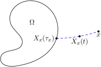
Figure 1. The curve $X_{x}(t)$ of (BC1) and the hitting time $\tau_{x}$.

Proof.

The proof is inspired by an argument of G. Barles, S. Mirrahimi, B. Perthame and P.E. Souganidis [8]. We only prove (a) since the proof of (b) is similar. Let $t\in(0,\tau_{y}]$ and define

$$w(s):=u(X_{y}(t-s))\quad\text{for }s\geq 0.$$

If we can prove that the usc function $w$ is a subsolution of

$$\frac{dw}{ds}(s)=g(X_{y}(t-s))\quad\text{for }s>0,$$ (2.3)

then by the comparison principle

$$w(s)\leq w(0)+\int_{0}^{s}g(X_{y}(t-\tau))d\tau\quad\text{for }s>0,$$

since the right-hand side is the $C^{1}$-solution of (2.3) with same initial data $w(0)$. Now (2.1) follows by choosing $s=t$.

To prove that $w$ is a supersolution of (2.3), we take any smooth test-function $\varphi$ and any point $\bar{s}>0$ such that $w-\varphi$ has a local strict maximum point at $\bar{s}$. Note that $X_{y}(t-\bar{s})\in\overline{\Omega}^{c}$ since $\bar{s}>0$. Next we introduce the functions

$$\phi(x,s)=\frac{|X_{y}(t-s)-x|^{2}}{\varepsilon^{2}}+\varphi(s)\qquad\text{and}\qquad\psi(x,s)=u(x)-\phi(x,s).$$

For $\varepsilon>0$ small enough, classical arguments show that $\psi$ has a maximum point near $(X_{y}(t-\bar{s}),\bar{s})$ (depending on $\varepsilon$) that we also call $(x,s)$. Moreover

$$\frac{|X_{y}(t-s)-x|^{2}}{\varepsilon^{2}}\rightarrow 0\quad\text{and}\quad s\rightarrow\bar{s}\qquad\text{as}\qquad\varepsilon\rightarrow 0.$$ (2.4)

Therefore $x\in\overline{\Omega}^{c}$ for $\varepsilon$ small enough, and since $u$ is a subsolution of (1.2) and $u-\phi(\cdot,t)$ has a local maximum at $x$,

$$-\frac{2(X_{y}(t-s)-x)}{\varepsilon^{2}}\cdot\gamma(x)\leq g(x).$$

Since $\tau\mapsto\psi(x,\tau)$ is a $C^{1}$-function having a local maximum at $\tau=s$, we also have

$$\frac{2(X_{y}(t-s)-x)}{\varepsilon^{2}}\cdot\dot{X}_{y}(t-s)-\dot{\varphi}(s)=\frac{\partial\psi}{\partial t}(x,s)=0,$$

and we can conclude using $\dot{X}_{y}(t-s)=-\gamma(X_{y}(t-s))$ and Lipschitz continuity of $\gamma$ that

$$\dot{\varphi}(s)= -\frac{2(X_{y}(t-s)-x)}{\varepsilon^{2}}\cdot\gamma(X_{y}(t-s))$$

$$\leq -\frac{2(X_{y}(t-s)-x)}{\varepsilon^{2}}\cdot\gamma(x)-\frac{2(X_{y}(t-s)-x)}{\varepsilon^{2}}\cdot\left(\gamma(X_{y}(t-s))-\gamma(x)\right)$$

$$\leq \ \ g(x)+O\Big{(}\frac{|X_{y}(t-s)-x|^{2}}{\varepsilon^{2}}\Big{)}\;.$$ (2.5)

In view of (2.4), we can send $\varepsilon\rightarrow 0$ to find that $\dot{\varphi}(\bar{s})\leq g(X_{y}(t-\bar{s}))$. ∎

To allow for convex domains with corners and $\gamma=n$, we need to relax the Lipschitz assumption on $\gamma$ in (BC1) and impose only a one-sided Lipschitz condition

• The functions $\gamma:\overline{\Omega}^{c}\to{\mathbb{R}}^{N}$ and $g:\overline{\Omega}^{c}\to{\mathbb{R}}$ are bounded continuous functions,

  $$(\gamma(x)-\gamma(y))\cdot(x-y)\geq-K|x-y|^{2}\;,$$ (2.6)

  for some constant $K$ and for all $x,y\in\overline{\Omega}^{c}$, and there exists $\nu>0$ such that $\gamma(x)\cdot n(x)\geq\nu$ for any $x\in\partial\Omega$.

We state a slight generalization of Lemma 2.1.

Lemma 2.2.

The results of Lemma 2.1 remain valid if we replace (BC1) by (BC1’).

Proof.

We first remark that (BC1’) ensures the existence and uniqueness of the trajectory $X_{y}$ as long as it remains in $\overline{\Omega}^{c}$, existence follows from Peano’s Theorem while (2.6) provides the uniqueness. Therefore the trajectory exists on $[0,\tau_{y})$ and can be extended by continuity to $t=\tau_{y}$.

To complete the proof, we let $t<\tau_{y}$ and redo the proof of Lemma 2.1. The computations are exactly the same, e.g. to obtain (2.5), (BC1’) is sufficient. To extend the result to $t=\tau_{y}$, we just remark that

$$\limsup_{t\uparrow\tau_{y}}u(X_{y}(t))\leq u(X_{y}(\tau_{y}))\;,$$

by the upper-semicontinuity of $u$. ∎

We conclude this section by an important discussion on the consequences of Lemma 2.1. If $u$ is a solution of (1.1)-(1.2), then $Du(x)\cdot\gamma(x)=g(x)$ in $\overline{\Omega}^{c}$ and we have, for all $y\in\overline{\Omega}^{c}$

$$u(y)=\int_{0}^{\tau_{y}}g(X_{y}(s))ds+u(X_{y}(\tau_{y})).$$

If $g\equiv 0$ on $\overline{\Omega}^{c}$, then $u$ can be bounded under suitable assumptions on the (other) data. This is the case we face in Section 3 below for convex domains and extended homogeneous Neumann boundary conditions. But if $g$ is not identically $0$ on $\overline{\Omega}^{c}$, then $u$ can be unbounded and its growth is governed by the properties of $g$ and $\tau_{y}$.

The behavior of $u$ at infinity is important in our framework to insure that the nonlocal terms are well-defined: We need some integrability property like e.g., for any $x\in\overline{\Omega}$ and $\delta>0$,

$$\int_{|z|\geq\delta}|u(x+j(x,z))|\,d\mu(z)<+\infty.$$ (2.7)

Such condition now connects the assumptions we have to place on $\tau_{x}$, $g$, $j$ and $\mu$.

To fix ideas, we are going to assume in Section 5.2 that:

• Either the function $g$ has a compact support in ${\mathbb{R}}^{N}$ or there exists $\tilde{c}>0$ such that for $\tau_{x}$ from (BC2),

  $$\tau_{x}\leq\tilde{c}(1+|x|)\qquad\hbox{and}\qquad\sup_{x\in\overline{\Omega}}\int_{|z|\geq\delta}|j(x,z)|\ d\mu(z)<\infty\ \hbox{for any $\delta>0$}\;.$$ (2.8)

We briefly comment on this assumption. When $g$ has compact support, the solutions are expected to be bounded by Lemma 2.1 and no additional assumption on $j$ and $\mu$ is needed. On the contrary, if e.g. $g\equiv 1$, then the integral of $g$ in (2.1) suggests that $u$ and $\tau_{x}$ have the same growth and (BC3) imposes a linear growth. Next one has to impose suitable hypothesis on $j$ and $\mu$ to satisfy (2.7). This is obtained through the second part of (BC3) on the $\mu$-integrability of $j$ away from $0$.

3. The homogeneous Neumann condition in convex non-smooth domains

In this section we consider the homogeneous Neumann problem, namely equation (1.1) and boundary condition (1.2) with $g\equiv 0$ and $\gamma=n$, the unit outward normal vector field in $\Omega^{c}$ (see below)

$$Du(x)\cdot n(x)=\ 0\quad\text{in}\quad\Omega^{c},$$ (3.1)

in the case when $\Omega$ is a convex, possibly unbounded and non-smooth domain.

At $x\in\partial\Omega$, the set of outward normals $N_{\Omega}(x)$ can be defined as

$$N_{\Omega}(x):=\Big{\{}n\in{\mathbb{R}}^{N}:|n|=1,n\cdot(x-y)\geq 0\text{ for all }y\in\overline{\Omega}\Big{\}}.$$

This set is a singleton at any point where $\partial\Omega$ is $C^{1}$ and part of a convex cone where $\partial\Omega$ has a corner. Let $\bar{d}$ be the distance function to $\overline{\Omega}$, and note that $\bar{d}\equiv 0$ in $\bar{\Omega}$ and $\bar{d}>0$ in $\overline{\Omega}^{c}$. Moreover, $\bar{d}$ is convex and belongs to $C^{0}({\mathbb{R}}^{N})\cap C^{1}(\overline{\Omega}^{c})$ since $\overline{\Omega}$ is a closed convex subset of ${\mathbb{R}}^{N}$. In $\bar{\Omega}^{c}$, we now define the outward unit normal vector $n$ in the only natural way by setting $n=D\bar{d}$. Note that the two definitions are consistent in the sense that

$$N_{\Omega}(x)=\Big{\{}n\in{\mathbb{R}}^{N}:n=\lim_{k\rightarrow\infty}D\bar{d}(x_{k})\text{ for some $x_{k}\rightarrow x$}\Big{\}}\quad\text{for all}\quad x\in\partial\Omega,$$

and since $\bar{d}$ is convex, the function $n$ satisfies (BC1’) with $K=0$.

To define the concept of viscosity solutions for this problem, we need the operators ${\mathcal{I}}_{\delta}$, ${\mathcal{I}}^{\delta}$, and $\mathcal{F}$ defined as follows

$${\mathcal{I}}_{\delta}[\phi](x)=\int_{|z|<\delta}\phi(x+j(x,z))-\phi(x)-D\phi(x)\cdot j(x,z)1_{B}(z)\,d\mu(z),$$

$${\mathcal{I}}^{\delta}[u](x)=\int_{|z|\geq\delta}u(x+j(x,z))-u(x)-D\phi(x)\cdot j(x,z)1_{B}(z)\,d\mu(z),$$

$$\mathcal{F}[u,\phi](x)=F(x,u(x),D\phi(x),D^{2}\phi(x),{\mathcal{I}}_{\delta}[\phi](x)+{\mathcal{I}}^{\delta}[u](x)).$$

Under assumption (1.5), ${\mathcal{I}}_{\delta}[\phi]$ is well-defined for $\phi\in C^{2}$. For ${\mathcal{I}}^{\delta}[u]$ we need some integrability condition a la (2.7), see the discussion at the end of Section 2. In this section $g\equiv 0$ on $\overline{\Omega}^{c}$, so (2.7) will be automatically satisfied whenever $u$ is bounded.

Definition 3.1.

(i) A locally bounded, usc function $u:{\mathbb{R}}^{N}\to{\mathbb{R}}$ is a viscosity subsolution of (1.1)–(1.2) if it satisfies (2.7), and for any test function $\phi\in C^{2}({\mathbb{R}}^{N})$ and for any maximum point $x_{0}\in{\mathbb{R}}^{N}$ of $u-\phi$ in $B_{c(j)\delta}(x_{0})$ where $c(j)$ is defined in (1.5), we have

$$\begin{cases}\mathcal{F}[u,\phi](x_{0})\leq 0&\hbox{if}\quad x_{0}\in\Omega,\\[5.69046pt] \displaystyle\min\bigg{(}\mathcal{F}[u,\phi](x_{0}),\inf_{n\in N_{\Omega}(x_{0})}D\phi(x_{0})\cdot n\bigg{)}\leq 0&\hbox{if}\quad x_{0}\in\partial\Omega,\\[5.69046pt] D\phi(x_{0})\cdot n(x_{0})\leq 0&\hbox{if}\quad x_{0}\in\overline{\Omega}^{c}\end{cases}$$

(ii) A locally bounded, lsc function $v:{\mathbb{R}}^{N}\to{\mathbb{R}}$ is a viscosity supersolution of (1.1)–(1.2) if it satisfies (2.7), and for any test function $\phi\in C^{2}({\mathbb{R}}^{N})$ and for any minimum point $x_{0}\in{\mathbb{R}}^{N}$ of the function $u-\phi$ in $B_{c(j)\delta}(x_{0})$ where $c(j)$ is defined in (1.5), we have

$$\begin{cases}\mathcal{F}[u,\phi](x_{0})\geq 0&\hbox{if}\quad x_{0}\in\Omega,\\[5.69046pt] \displaystyle\max\bigg{(}\mathcal{F}[u,\phi](x_{0}),\sup_{n\in N_{\Omega}(x_{0})}D\phi(x_{0})\cdot n\bigg{)}\geq 0&\hbox{if}\quad x_{0}\in\partial\Omega,\\[5.69046pt] D\phi(x_{0})\cdot n(x_{0})\geq 0&\hbox{if}\quad x_{0}\in\overline{\Omega}^{c}\end{cases}$$

(iii) A viscosity solution $u$ of (1.1)–(1.2) is a locally bounded function whose upper and lower semicontinuous envelopes are respectively sub- and supersolution of the problem.

This definition is a natural extension of the definition given in [5] to the Neumann type boundary value problem.

Remark 3.2.

Two useful equivalent definitions can be given: (1) We can replace ${\mathcal{I}}^{\delta}[u]$ by ${\mathcal{I}}^{\delta}[\phi]$ in the above definition if local maximum/minimum points are replaced by global ones. (2) In the subsolution definition, $(D\phi(x_{0}),D^{2}\phi(x_{0}))$ can be replaced by elements $(p,X)$ in the so-called super-jet $J^{+}u(x_{0})$ if $X\leq D^{2}\phi(x_{0})$. In the definition of supersolutions, you can similarly use $(q,Y)\in J^{-}u(x_{0})$ if $Y\geq D^{2}\phi(x_{0})$. The second definition is useful for comparison proofs, and the proofs of these claims easily follow from the arguments for similar results in [6].

We now state the assumptions – remarking that the assumptions on $F$ will be as general as for the whole space case $\Omega={\mathbb{R}}^{N}$ without boundary conditions. For convenience we use the assumptions of [6], but see Remark 3.6 below for more general assumptions. For the nonlocal part we assume that

• Assumption (1.5) holds, and there is a constant $\bar{c}>0$ such that for all $x,y\in{\mathbb{R}}^{N}$,

  $$\int_{{\mathbb{R}}^{N}}\frac{|j(x,z)-j(y,z)|^{2}}{|x-y|^{2}}+\int_{{\mathbb{R}}^{N}\setminus B}\frac{|j(x,z)-j(y,z)|}{|x-y|}\mu(dz)\leq{\bar{c}}.$$

The non-linearity $F$ satisfies the following classical assumptions

• There exists ${\lambda_{0}}>0$ such that for any $x\in{\mathbb{R}}^{d}$, $u,v\in{\mathbb{R}}$, $p\in{\mathbb{R}}^{d}$, $X\in\mathbb{S}^{N}$ and $l\in{\mathbb{R}}$,

  $$F(x,u,p,X,l)-F(x,v,p,X,l)\geq{\lambda_{0}}(u-v)\quad\mbox{when}\quad u\geq v.$$

• $F$ is continuous, and for any $R>0$, there exist moduli of continuity $\omega,\omega_{R}$ such that, for any $|x|,|y|\leq R$, $|v|\leq R$, $l\in{\mathbb{R}}$ and for any $X,Y\in\mathbb{S}^{N}$ satisfying

  $$\left[\begin{array}[]{cc}X&0\\ 0&-Y\end{array}\right]\leq\frac{1}{\varepsilon}\left[\begin{array}[]{cc}I&-I\\ -I&I\end{array}\right]+r(\beta)\left[\begin{array}[]{cc}I&0\\ 0&I\end{array}\right]$$ (3.2)

  for some $\varepsilon>0$ and $r(\beta)\to 0$ as $\beta\to 0$, then, if $s_{i}(\beta)\to 0$ as $\beta\to 0$ for $i=1$ and $2$, we have

  $$\begin{split}&F(y,v,\varepsilon^{-1}(x-y)+s_{1}(\beta),Y,l)-F(x,v,\varepsilon^{-1}(x-y)+s_{2}(\beta),X,l)\\ &\leq\omega(\beta)+\omega_{R}(|x-y|+\varepsilon^{-1}|x-y|^{2}).\end{split}$$ (3.3)

• For any $R>0$, $F$ is uniformly continuous on ${\mathbb{R}}^{n}\times[-R,R]\times B_{R}\times D_{R}\times{\mathbb{R}}$ where $D_{R}:=\{X\in\mathbb{S}^{N};\ |X|\leq R\}$ and there exist a modulus of continuity $\omega_{R}$ such that, for any $x,y\in{\mathbb{R}}^{d}$, $|v|\leq R$,$l\in{\mathbb{R}}$ and for any $X,Y\in\mathbb{S}^{N}$ satisfying (3.2) and $\varepsilon>0$, we have

  $$F(y,v,\varepsilon^{-1}(x-y),Y,l)-F(x,v,\varepsilon^{-1}(x-y),X,l)\leq\omega_{R}(\varepsilon^{-1}|x-y|^{2}+|x-y|).$$ (3.4)

• $F(x,u,p,X,l)$ is nondecreasing and Lipschitz continuous in $l$, uniformly with respect to all the other variables.

• $M_{F}:=\sup_{x\in\Omega}|F(x,0,0,0,0)|<\infty.$

Assumption (A3-1) and (A3-2) are two versions of assumption (3.14) in the Users’ Guide [12] for possibly unbounded domains. These assumptions along with (A4) imply that equation (1.1) is degenerate elliptic. Assumptions (A3-1) allows more general $x$-dependence in the equation (e.g. HJB equations with at most linear growth in the derivatives and general $x$-depending coefficients), while (A3-2) allows more general gradient dependence in the equation (e.g. HJB equations with coefficients which are bounded in $x$ but possibly with $x$-independent superlinear gradient terms).

To be more explicit, consider the linear equation (1.6). The above assumptions hold if $a\geq 0$, $A(x)=\sigma(x)\sigma^{T}(x)$ for some matrix $\sigma$, and, for (A2), $\lambda(x)\geq\lambda_{0}>0$ in ${\mathbb{R}}^{N}$. Assumptions (A3-1) and (A3-2) are the following two variants of conditions on $\sigma,b,\lambda,f$: (A3-1) is satisfied if $\sigma$ and $b$ are bounded and locally Lipschitz continuous and $\lambda$ and $f$ are continuous. For (A3-2), $\sigma$, $b$ can have a linear growth but one needs the global Lipschitz continuity of $\sigma$ and $b$, and the uniform continuity of $\lambda$ and $f$.

In the local case with no ${\mathcal{I}}$-dependence in the equation, assumptions (A2) – (A5) imply comparison, uniqueness, and existence (via Perron’s method) of a bounded viscosity solution of (1.1)–(1.2), cf. e.g. [12]. In the nonlocal case when $\Omega={\mathbb{R}}^{N}$ (and no Neumann conditions, $\Omega^{c}=\emptyset$), we have the following rather classical result which we will need later.

Proposition 3.3 (Results for $\Omega={\mathbb{R}}^{N}$).

Assume $\Omega={\mathbb{R}}^{N}$ and (A1), (A2), (A4) hold along with either (A3-1) or (A3-2).

(a) If $u$ and $v$ are respectively an usc bounded above subsolution and a lsc bounded below supersolution of (1.1) in $\Omega={\mathbb{R}}^{N}$, then $u\leq v$ in ${\mathbb{R}}^{N}$.

(b) Assume also (A5) holds, then there exists a unique bounded viscosity solution $u$ of (1.1) in $\Omega={\mathbb{R}}^{N}$ satisfying

$$|u(x)|\leq\frac{M_{F}}{{\lambda_{0}}}\quad\text{in}\quad{\mathbb{R}}^{N}.$$ (3.5)

Part (a) was proved in [6] (see Section 5), and Part (b) follows from part (a) and Perron’s method since $M_{F}/{\lambda_{0}}$ and $-M_{F}/{\lambda_{0}}$ are super and subsolutions of (1.1). Similar results have been given e.g. in [3, 24, 19, 5].

Now we come to the first main result of this paper, a comparison result for the boundary value problem (1.1)–(3.1).

Theorem 3.4 (Comparison I).

Assume (A1), (A2), (A4) hold along with either (A3-1) or (A3-2). If $u$ and $v$ are respectively an usc bounded above subsolution and a lsc bounded below supersolution of (1.1)–(3.1), then $u\leq v$ in ${\mathbb{R}}^{N}$.

Uniqueness of solutions follow, and since $\pm\frac{M_{F}}{{\lambda_{0}}}$ are sub/super solutions of (1.1) when (A5) holds, we also get $L^{\infty}$-bounds.

Corollary 3.5.

Assume (A1), (A2), (A4) hold along with either (A3-1) or (A3-2).​​​​​

(a) There is not more than one bounded solution of (1.1).

(b) If also (A5) holds, then any solution $u$ of (1.1) satisfies (3.5).

Remark 3.6.

Under assumption (A3-1), the above results also holds if assumption (A1) is replaced by the much more general assumption:

• Assumption (1.5) holds and there exists a constant $\bar{c}>0$ such that

  $$\int_{B}|j(x,z)-j(y,z)|^{2}\mu(dz)\leq{\bar{c}}|x-y|^{2}.$$

The proof in Section 5 in [6] can be modified easily to cover this case by a clever trick which can be found e.g. in Section 6 in [19]. Compared to assumption (A1), assumption (A1-2) allows more general dependences of $j(x,z)$ in $x$. If we also relax (1.5) so that the constant $c(j)$ is finite only for compact subsets of $x\in\Omega$, then the above results also cover the case when $j$ has linear growth in $x$.

Figure 2. The curves of (BC1) with $\gamma=n$ starting at $y_{1}$ and $y_{2}$ and ending at a corner point of $\partial\Omega$.

Proof of Theorem 3.4.

We introduce the following initial value problem (cf. (BC2)),

$$\dot{X}_{y}(t)=-n(X_{y}(t))\ \ \text{for}\ \ t>0,\qquad X_{y}(0)=y.$$ (3.6)

Note that the projection on the closed convex set $\overline{\Omega}$, $P:\Omega^{c}\rightarrow\partial\Omega$, is also given by

$$P_{y}=X_{y}(\tau_{y})\quad\hbox{for any }y\in\overline{\Omega}^{c}\;,$$

where we recall that

$$\tau_{y}=\inf\{t>0:X_{y}(t)\in\partial\Omega\}.$$

Since $\Omega$ is convex and $|n|=1$, it follows that $\{X_{y}(\cdot)\}_{y}$ defines a family of constant speed, finite length, and non-intersecting paths in $\overline{\Omega}^{c}$ having the form

$$X_{y}(t)=y-tn(y)\quad\text{for}\quad t\in[0,\tau_{y}].$$ (3.7)

Obviously $\tau_{y}<\infty$ for all $y$ so that (BC2) is trivially satisfied when $\gamma=n$.

We argue by contradiction assuming that

$${M:=\sup_{{\mathbb{R}}^{N}}\{u(x)-v(x)\}>0}.$$

Since $n$ satisfies (BC1’), Lemma 2.2 applies with $g\equiv 0$ and we find that $u(x)-v(x)\leq u(P_{x})-v(P_{x})$ in $\overline{\Omega}^{c}$, and hence that $\displaystyle{M=\max_{\overline{\Omega}}\{u(x)-v(x)\}}$.

Let $\chi:{\mathbb{R}}\to{\mathbb{R}}$ be a bounded smooth function such that $\chi(t)\equiv 0$ for $t\leq 0$, $\chi^{\prime}(t)>0$ for $t>0$, and $\chi(t)\geq 2(||u||_{\infty}+||v||_{\infty})$ for $t\geq 1$. We double the variables, introducing the function

$$\Psi(x,y)=u(x)-v(y)-\frac{|x-y|^{2}}{\varepsilon^{2}}-\chi(\beta(|x-x_{0}|^{2}+1))-\chi(\beta(|y-x_{0}|^{2}+1)),$$

where $\varepsilon,\beta>0$, and $x_{0}$ is any given point in $\Omega$. It is easy to see that, for $\beta$ small enough, $M_{\varepsilon,\beta}=\max_{{\mathbb{R}}^{2N}}\Psi(x,y)$ exists and is attained at some point $(\bar{x},\bar{y})\in{\mathbb{R}}^{N}\times{\mathbb{R}}^{N}$ (that depends on $\varepsilon$ and $\beta$). The crucial and new step in the proof is to show that $(\bar{x},\bar{y})\in\bar{\Omega}\times\bar{\Omega}$. If this was not the case, then two applications of Lemma 2.2 yields that

$$u(\bar{x})-v(\bar{y})\leq u(P_{\bar{x}})-v(P_{\bar{y}}).$$ (3.8)

Moreover, since $\Omega$ is convex and $x_{0}\in\Omega$,

$$|\bar{x}-\bar{y}|\geq|P_{\bar{x}}-P_{\bar{y}}|,\quad|{\bar{x}}-x_{0}|\geq|P_{\bar{x}}-x_{0}|,\quad\text{and}\quad|{\bar{y}}-x_{0}|\geq|P_{\bar{y}}-x_{0}|,$$ (3.9)

and then, for $\beta$ small enough, we have the contradiction

$$M_{\varepsilon,\beta}=\Psi(\bar{x},\bar{y})<\Psi(P_{\bar{x}},P_{\bar{y}}).$$ (3.10)

Since $\bar{x},\bar{y}\in\overline{\Omega}$, the rest of the proof follows classical arguments. Assume ${\bar{x}}\in\partial\Omega$ and let

$$\phi(x,y)=\frac{|x-y|^{2}}{\varepsilon^{2}}+\chi(\beta(|x-x_{0}|^{2}+1))+\chi(\beta(|y-x_{0}|^{2}+1)).$$

Note that by convexity of $\Omega$,

$$({\bar{x}}-y)\cdot n\geq 0\quad\text{for all}\quad y\in\overline{\Omega},\ n\in N_{\Omega}({\bar{x}}).$$

Moreover, this inequality is strict if $y\in\Omega$. Finally, since $\chi^{\prime}(t)>0$ for $t>0$, we use the fact that $x_{0}\in\Omega$ to find that

$$\begin{split}D_{x}\phi({\bar{x}},{\bar{y}})\cdot n&=\frac{2}{\varepsilon^{2}}({\bar{x}}-{\bar{y}})\cdot n+\chi^{\prime}(\beta(|{\bar{x}}-x_{0}|^{2}+1))2\beta({\bar{x}}-x_{0})\cdot n\\ &>0\qquad\text{for all}\qquad n\in N_{\Omega}({\bar{x}})\ \text{and}\ \beta>0.\end{split}$$ (3.11)

Therefore, from Definition 3.1, the equation has to hold at ${\bar{x}}$, i.e. $\mathcal{F}[u,\phi(\cdot,{\bar{y}})]({\bar{x}})\leq 0$. A similar argument shows that $\mathcal{F}[v,-\phi({\bar{x}},\cdot)]({\bar{y}})\geq 0$ if ${\bar{y}}\in\partial\Omega$.

Now we are in the situation that ${\bar{x}},{\bar{y}}\in\overline{\Omega}$ and that the equation is satisfied at these points. The conclusion of the proof is then exactly as for the ${\mathbb{R}}^{N}$ case, and we omit the standard details. Under the present assumptions, essentially all the remaining details can be found in Section 5 in [6]. But see also [3, 19, 24] for very similar results. ∎

Remark 3.7.

The key ingredients of the above proof are

• Inequality (3.8) that comes from Lemma 2.1 or 2.2 and that allow us to compare values of $u$ and $v$ outside $\overline{\Omega}$ with those on inside $\overline{\Omega}$.

• Inequality (3.10) that comes from convexity and contraction properties (see (3.9)). In the above proof, the contraction property of the projection on the closed, convex set $\overline{\Omega}$ was playing the key role (allowing us to use a very simple test function), but in general the contraction property comes from the control on the $X_{y}$ trajectories w.r.t. $y$.

• As in the classical Neumann/oblique derivatives boundary conditions cases, the test-function has to be build in order to allow us to “avoid” the boundary condition (cf. (3.11)).

These three ingredients are the same in any proof but with different arguments to handle them. We are going to focus on these arguments.

Remark 3.8.

If $\Omega$ is bounded, we can relax assumptions (A3-1) and (A3-2) in the standard way and the comparison result will still hold. E.g. since we no longer need to prevent maximum points from escaping to infinity, we can set all functions $r,s_{1},s_{2}$ and $\omega$ equal zero in (A3-1).

4. General oblique derivative conditions in non-convex smooth domains

In this section we consider the general oblique derivative problem of the form (1.1)–(1.2) on a bounded, possibly non-convex , $C^{2}$-domain $\Omega$. Compared to section 3, the domain and boundary condition and are more general, but the class of equations (see below) and the boundary regularity are more restricted.

Assuming that (1.5) and (BC1) hold, and we now have the following definition of viscosity solutions

Definition 4.1.

(i) A locally bounded, usc function $u:{\mathbb{R}}^{N}\to{\mathbb{R}}$ is a viscosity subsolution of (1.1)–(1.2) if it satisfies (2.7), and for any test function $\phi\in C^{2}({\mathbb{R}}^{N})$ and for any maximum point $x_{0}\in{\mathbb{R}}^{N}$ of $u-\phi$ in $B_{c(j)\delta}(x_{0})$ where $c(j)$ is defined in (1.5),

$$\begin{cases}\mathcal{F}[u,\phi](x_{0})\leq 0&\hbox{if}\quad x_{0}\in\Omega,\\[5.69046pt] \displaystyle\min\bigg{(}\mathcal{F}[u,\phi](x_{0}),D\phi(x_{0})\cdot\gamma(x_{0})-g(x_{0})\bigg{)}\leq 0&\hbox{if}\quad x_{0}\in\partial\Omega,\\[5.69046pt] D\phi(x_{0})\cdot\gamma(x_{0})\leq g(x_{0})&\hbox{if}\quad x_{0}\in\overline{\Omega}^{c}\end{cases}$$

(ii) A locally bounded, lsc function $v:{\mathbb{R}}^{N}\to{\mathbb{R}}$ is a viscosity supersolution of (1.1)–(1.2) if it satisfies (2.7), and for any test function $\phi\in C^{2}({\mathbb{R}}^{N})$ and for any minimum point $x_{0}\in{\mathbb{R}}^{N}$ of the function $u-\phi$ in $B_{c(j)\delta}(x_{0})$ where $c(j)$ is defined in (1.5),

$$\begin{cases}\mathcal{F}[u,\phi](x_{0})\geq 0&\hbox{if}\quad x_{0}\in\Omega,\\[5.69046pt] \displaystyle\max\bigg{(}\mathcal{F}[u,\phi](x_{0}),D\phi(x_{0})\cdot\gamma(x_{0})-g(x_{0})\bigg{)}\geq 0&\hbox{if}\quad x_{0}\in\partial\Omega,\\[5.69046pt] D\phi(x_{0})\cdot\gamma(x_{0})\geq g(x_{0})&\hbox{if}\quad x_{0}\in\overline{\Omega}^{c}\end{cases}$$

(iii) A viscosity solution $u$ of (1.1)–(1.2) is a locally bounded function whose upper and lower semicontinuous envelopes are respectively sub- and supersolution of the problem.

To handle non-convex domains and more general boundary conditions, we will use a rather complicated test-function which is no longer only a function of $x-y$ plus small terms. For the proofs to work out we therefore need to replace assumption (A3-1) and (A3-2) by a more restrictive assumption similar to the one used in the local case [2]

• For any $R,K>0$, there exist moduli of continuity $m_{R,K}$ such that, for any $x,y\in\overline{\Omega}$, $|u|\leq R$, $p,q\in{\mathbb{R}}^{N}$, $l\in{\mathbb{R}}$, and matrices $X,Y\in\mathbb{S}^{N}$ satisfying

  $$|x-y|\leq\eta\varepsilon,\qquad|p-q|\leq K\eta\varepsilon(1+|p|\wedge|q|),\quad\text{and}$$

  $$-\frac{K}{\varepsilon^{2}}Id\leq\left(\begin{array}[]{cc}X&0\\ 0&-Y\end{array}\right)\leq\frac{K}{\varepsilon^{2}}\left(\begin{array}[]{cc}Id&-Id\\ -Id&Id\end{array}\right)+K\eta Id,$$

  we have that

  $$F(y,u,q,Y,l)-F(x,u,p,X,l)\leq m_{R,K}\left(\eta+|x-y|(1+|p|\vee|q|)+\frac{|x-y|^{2}}{\varepsilon^{2}}\right).$$

We have the following comparison result.

Theorem 4.2 (Comparison II).

Assume (A1), (A2), (A3-3), (A4), (BC1), and (BC2) hold. If $u$ and $v$ are respectively a locally bounded usc subsolution and a locally bounded lsc supersolution of (1.1)–(1.2), then $u\leq v$ in ${\mathbb{R}}^{N}$.

This result will be proved in the subsections below. We start by introducing the test function we need for the proof.

4.1. The test-function

As for local oblique derivative boundary conditions (see e.g. [2] and references therein), the proof of our comparison result requires a rather complicated test-function. Fortunately there are no major differences between the test-function for the local and nonlocal cases, and we now recall a few facts about the test-function of [2] and describe the adaptations we need to make here.

We start by changing our definition of the “distance to the boundary” $d$. Now $d$ will be a bounded $C^{2}$ function which is equal to the signed distance function to $\partial\Omega$ in a neighborhood of $\partial\Omega$ ($d>0$ in $\Omega$ and  $d<0$ in $\overline{\Omega}^{c}$) and where $n(x):=-Dd(x)\neq 0$ in $\Omega^{c}$. Note that $n(x)$ is the outward unit normal vector to $\partial\Omega$ for any $x\in\partial\Omega$. The test-function $\psi_{\varepsilon,\eta}\in C^{2}({\mathbb{R}}^{2N})$ of [2] can then be defined as follows,

$$\psi_{\varepsilon,\eta}(x,y)= \ e^{-K_{1}[d(x)+d(y)]}\,{{|x-y|^{2}}\over{\varepsilon^{2}}}$$

$$-C_{\eta\varepsilon}\Big{(}\frac{x+y}{2},e^{-K_{1}[d(x)+d(y)]}\,{{2(x-y)}\over{\varepsilon^{2}}}\Big{)}\big{(}d(x)-d(y)\big{)}$$ (4.1)

$$+e^{-K_{1}[d(x)+d(y)]}\,{{A\big{(}d(x)-d(y)\big{)}^{2}}\over{\varepsilon^{2}}}-K_{2}\eta\varepsilon\,[d(x)+d(y)]\;,$$

for parameters $\eta,\varepsilon>0$ (small), constants $A,K_{1},K_{2}$ (large), and where the function $C_{\eta\varepsilon}$ (see [2] page 214) is a suitable smooth approximation of a bounded Lipschitz extension of the solution $t=C(x,p)$ of the equation

$$\gamma(x)\cdot(p+tn(x))-g(x)=0\qquad\text{for}\qquad p\in{\mathbb{R}}^{N},\ x\text{ near }\partial\Omega.$$

The key properties of the test-function are given in the Lemma below.

Lemma 4.3.

Assume (BC1) and let $R>0$. If $\eta,\varepsilon>0$ are small enough, then for $A,K_{1},K_{2}$ large enough, then the function $\psi_{\varepsilon,\eta}$ defined in (4.1) has the following properties

(i) For any $x,y\in{\mathbb{R}}^{N}$,

$$\psi_{\varepsilon,\eta}(x,y)\geq K^{-1}{{|x-y|^{2}}\over{\varepsilon^{2}}}-K\varepsilon^{2}-K_{2}\eta\varepsilon\,[d(x)+d(y)].$$ (4.2)

(ii) For $\varepsilon,\eta\in(0,1)$ and $|x-y|\leq\eta\varepsilon$,

$$|D_{x}\psi_{\varepsilon,\eta}(x,y)|+|D_{y}\psi_{\varepsilon,\eta}(x,y)|\geq-K+K^{-1}{{|x-y|}\over{\varepsilon^{2}}},$$

$$|D_{x}\psi_{\varepsilon,\eta}(x,y)|+|D_{y}\psi_{\varepsilon,\eta}(x,y)|\leq$$

$$\quad C{{|x-y|}\over{\varepsilon^{2}}}+C\Big{(}1+\eta^{2}K_{1}e^{2K_{1}\|d\|_{\infty}}+\varepsilon\eta K_{2}\Big{)},$$ (4.3)

$$|D_{x}\psi_{\varepsilon,\eta}(x,y)+D_{y}\psi_{\varepsilon,\eta}(x,y)|\leq K{{|x-y|^{2}}\over{\varepsilon^{2}}}+K(\eta\varepsilon+\varepsilon^{2}),\text{ and}$$

$$\frac{K}{\varepsilon^{2}}Id\leq D^{2}\psi_{\varepsilon,\eta}(x,y)\leq\frac{K}{\varepsilon^{2}}\left(\begin{array}[]{cc}Id&-Id\\ -Id&Id\end{array}\right)+K\eta Id.$$ (4.6)

(iii) There is $\delta>0$ such that for $|x-y|\leq\delta$ and $x,y$ in a neighborhood of $\partial\Omega$,

$$\gamma(x)\cdot D_{x}\psi_{\varepsilon,\eta}(x,y)) >g(x)\quad\hbox{if }d(x)\leq d(y)\;,$$ (4.7)

$$-\gamma(y)\cdot D_{y}\psi_{\varepsilon,\eta}(x,y)) <g(y)\quad\hbox{if }d(y)\leq d(x)\;,$$ (4.8)

and if in addition $|x-y|\leq\eta\varepsilon$, then

$$\begin{split}&-\gamma(x)\cdot\big{(}D_{x}\psi_{\varepsilon,\eta}(x,y)+D_{y}\psi_{\varepsilon,\eta}(x,y)\big{)}\\ &\leq-K_{1}\frac{\nu}{4}e^{-K_{1}[d(x)+d(y)]}{{|x-y|^{2}}\over{\varepsilon^{2}}}-K_{2}\frac{\nu}{4}\eta\varepsilon.\end{split}$$ (4.9)

Except for (4.9), these estimates have essentially been proved in Section 5 in [2]. Some new features that only marginally changes the proofs are: (i) $x,y$ can now belong to $\Omega^{c}$, (ii) inequality (4.2) is slightly more accurate, and (iii) inequalities (4.7) and (4.8) are now given in a neighborhood and not only at $\partial\Omega$. Moreover, the constants $K$ will in general depend on $K_{1}$ and $K_{2}$, and the precise dependence is not important except for the term (4.3). The importance of this dependence is both new and central to this paper (cf. the proof of Lemma 4.4 a)). We will therefore prove both (4.3) and (4.9) here.

Proof of (4.3) and (4.9).

To simplify the computations, we write $\psi_{\varepsilon,\eta}$ in the following way

$$\psi_{\varepsilon,\eta}(x,y)=\chi(x-y,d(x)-d(y),\frac{x+y}{2},d(x)+d(y))\;,$$

where

$$\chi(X,Y,Z,T):=e^{-K_{1}T}{{X^{2}}\over{\varepsilon^{2}}}-C_{\eta\varepsilon}\left(Z,e^{-K_{1}T}{{2X}\over{\varepsilon^{2}}}\right)Y+e^{-K_{1}T}{{AY^{2}}\over{\varepsilon^{2}}}-K_{2}\eta\varepsilon T\;.$$

In this notation,

$$D_{x}\psi_{\varepsilon,\eta}(x,y)=\chi_{X}-\chi_{Y}n(x)+\frac{1}{2}\chi_{Z}-\chi_{T}n(x),$$

$$D_{x}\psi_{\varepsilon,\eta}(x,y)+D_{y}\psi_{\varepsilon,\eta}(x,y)=-\chi_{Y}(n(x)-n(y))+\chi_{Z}-\chi_{T}(n(x)+n(y)).$$

By the assumptions on $\gamma$ and $g$ and the construction of $C_{\eta\varepsilon}=C_{\eta\varepsilon}(x,p)$ in [2], there is a $C>0$ such that

$$|C_{\varepsilon\eta}|+|D_{x}C_{\varepsilon\eta}|\leq C(1+|p|)\qquad\text{and}\qquad|D_{p}C_{\varepsilon\eta}|\leq C.$$

Hence there are constants $C_{1}$ and $C_{2}$ such that

$$|\chi_{X}|+|\chi_{Y}| \leq C_{1}+C_{2}e^{-K_{1}T}\Big{(}{{2|X|}\over{\varepsilon^{2}}}+{{2(1+A)|Y|}\over{\varepsilon^{2}}}\Big{)},$$

$$|\chi_{Z}| \leq\Big{(}C_{1}+C_{2}e^{-K_{1}T}{{2|X|}\over{\varepsilon^{2}}}\Big{)}|Y|,$$

$$|\chi_{T}| \leq K_{1}e^{-K_{1}T}C_{2}\Big{(}{{X^{2}}\over{\varepsilon^{2}}}+{{(1+A)Y^{2}}\over{\varepsilon^{2}}}\Big{)}+K_{2}\eta\varepsilon.$$

Since $|X|,|Y|\leq C|x-y|$, estimate (4.3) now follows.

To prove (4.9), we note that by using Cauchy-Schwarz inequality on the $D_{p}C_{\varepsilon\eta}$-term and taking $A$ large enough,

$$\chi_{T} =-K_{1}e^{-K_{1}T}\left[{{X^{2}}\over{\varepsilon^{2}}}-D_{p}C_{\eta\varepsilon}\cdot{{2X}\over{\varepsilon^{2}}}Y+{{AY^{2}}\over{\varepsilon^{2}}}\right]-K_{2}\eta\varepsilon$$

$$\leq-\frac{K_{1}}{2}e^{-K_{1}T}\Big{(}{{X^{2}}\over{\varepsilon^{2}}}+{{AY^{2}}\over{\varepsilon^{2}}}\Big{)}-K_{2}\eta\varepsilon.$$

Let $\mathcal{W}=\{x:\operatorname{dist}(x,\partial\Omega)<r\}$, and let $r>0$ be so small that $\gamma\cdot n\geq\frac{\nu}{2}$ in $\mathcal{W}$. Such a set exists by (BC1) and continuity of $\gamma$ and $n$. After an easy computation based on the above estimates, the Lipschitz continuity of $n$ ($|n(x)-n(y)|\sim|X|$), the inequality $\gamma\cdot n\geq\frac{\nu}{2}$, Cauchy-Schwarz inequality, and finally, taking $K_{1},K_{2}$ large enough so that the $\chi_{T}$-term dominates, we conclude that (4.9) holds in $\mathcal{W}$. ∎

The next lemma plays a key role in the comparison proof.

Lemma 4.4.

Assume (BC1) and (BC2), let $\tau_{x}$ be defined in Lemma 2.1, and $\tau:=\min(\tau_{x},\tau_{y})$.

(a) For any $\tilde{K}\geq 0$, there are constants $K_{1},K_{2}$ large enough, such that for any $\varepsilon,\eta>0$ small enough, if $x,y\in\Omega^{c}$ are close enough to $\partial\Omega$ and $|x-y|\leq\eta\varepsilon/2$, then

$$\psi_{\varepsilon,\eta}(X_{x}(\tau),X_{y}(\tau)) \leq\psi_{\varepsilon,\eta}(x,y)-\tilde{K}\tau\eta\varepsilon.$$ (4.10)

(b) For any $\eta>0$, there are constants $K_{1},K_{2}$ large enough, such that for any $\varepsilon>0$, if $x,y\in\Omega^{c}$ are close enough to $\partial\Omega$ and $\tau_{y}\leq\tau_{x}$, then

$$\psi_{\varepsilon,\eta}(X_{x}(\tau_{x}),X_{y}(\tau)) \leq\psi_{\varepsilon,\eta}(X_{x}(\tau),X_{y}(\tau))-\int_{\tau_{y}}^{\tau_{x}}g(X_{x}(t))dt.$$ (4.11)

(c) For any $\eta>0$, there are constants $K_{1},K_{2}$ large enough, such that for any $\varepsilon>0$, if $x\in\Omega^{c}$ and $y\in\overline{\Omega}$ are close enough to $\partial\Omega$, then

$$\psi_{\varepsilon,\eta}(X_{x}(\tau_{x}),y) \leq\psi_{\varepsilon,\eta}(x,y)-\int_{0}^{\tau_{x}}g(X_{x}(t))dt.$$

Figure 3. Curves of (BC1) with different starting points in the oblique case.

Proof.

Consider a neighborhood of $\partial\Omega$, $\mathcal{W}_{r}=\{x:\operatorname{dist}(x,\partial\Omega)<r\}$, and let $r>0$ be so small that (4.9) holds, $d(x)=\pm\operatorname{dist}(x,\partial\Omega)$, and $\gamma\cdot n\geq\frac{\nu}{2}$ in $\mathcal{W}_{r}$. Such a set exists by the definition of $d$, (BC1), and continuity of $\gamma$ and $n$. In the set $\mathcal{W}_{r}\cap\Omega^{c}$ the distance to boundary $f(t)=\operatorname{dist}(X_{x}(t),\partial\Omega)=-d(X_{x}(t))$ is decreasing,

$$\dot{f}(t)=-Dd(X_{x}(t))\cdot\dot{X}_{x}(t)=n(X_{x}(t))\cdot(-\gamma(X_{x}(t)))<-\frac{\nu}{2},$$ (4.12)

and hence $X_{x}(t)\in\mathcal{W}_{r}\cap\Omega^{c}$ for all $t\in[0,\tau_{x}]$ and $x\in\mathcal{W}_{r}\cap\Omega^{c}$.

Next we note that if $L$ is the Lipschitz constant of $\gamma$, then by Grönwall’s inequality,

$$|X_{x}(t)-X_{y}(t)|\leq e^{Lt}|x-y|.$$ (4.13)

We estimate $\tau_{x}$, and hence also $\tau_{y}$ and $\tau$, by integrating (4.12) from $t$ to $\tau_{x}$ and noting that $f(\tau_{x})=0$

$$\frac{\nu}{2}(\tau_{x}-t)<f(t)=\operatorname{dist}(X_{x}(t),\partial\Omega)\leq\operatorname{dist}(x,\partial\Omega)\quad\text{for}\quad t\in[0,\tau_{x}].$$

Hence if $r$ is small, $\tau$ will also be small in $\mathcal{W}_{r}\cap\Omega^{c}$. In the rest of the proof we take $x,y\in\mathcal{W}_{r}\cap\Omega^{c}$, and then we take $r$ so small that also $|X_{x}(t)-X_{y}(t)|\leq\eta\varepsilon$ for all $t\in[0,\tau]$ and $x,y\in\mathcal{W}_{r}\cap\Omega^{c}$ such that $|x-y|\leq\frac{\eta\varepsilon}{2}$.

We now prove part (a). We start by using the definition of $X_{x}(t)$ (see (BC2)) to show that

$$\frac{d}{dt}\left[\psi_{\varepsilon,\eta}(X_{x}(t),X_{y}(t))\right]=-D_{x}\psi_{\varepsilon,\eta}\cdot\gamma(X_{x}(t))-D_{y}\psi_{\varepsilon,\eta}\cdot\gamma(X_{y}(t))$$

$$=-[D_{x}\psi_{\varepsilon,\eta}+D_{y}\psi_{\varepsilon,\eta}]\cdot\gamma(X_{x}(t))-D_{y}\psi_{\varepsilon,\eta}\cdot[\gamma(X_{y}(t))-\gamma(X_{x}(t))].$$

We may use (4.3) (check!) and the Lipschitz continuity of $\gamma$ to have

$$|D_{y}\psi_{\varepsilon,\eta}\cdot[\gamma(X_{y}(t))-\gamma(X_{x}(t))]|$$

$$\leq L|X_{x}(t)-X_{y}(t)|\cdot C\Big{(}{{|X_{x}(t)-X_{y}(t)|}\over{\varepsilon^{2}}}+1+\eta^{2}K_{1}e^{K_{1}2\|d\|_{\infty}}+\varepsilon\eta K_{2}\Big{)}$$

$$\leq LC\Big{(}{{|X_{x}(t)-X_{y}(t)|^{2}}\over{\varepsilon^{2}}}+\eta\varepsilon\Big{(}1+\varepsilon\eta K_{2}+\eta^{2}K_{1}e^{2K_{1}\|d\|_{\infty}}\Big{)}\Big{)},$$

and by (4.9) we immediatly find that

$$-[D_{x}\psi_{\varepsilon,\eta}+D_{y}\psi_{\varepsilon,\eta}]\cdot\gamma(X_{x}(t))$$

$$\leq-K_{1}\frac{\nu}{4}\,e^{-K_{1}[d(X_{x}(t))+d(X_{y}(t))]}\,{\frac{|X_{x}(t)-X_{y}(t)|^{2}}{\varepsilon^{2}}}-K_{2}\frac{\nu}{4}\eta\varepsilon.$$

Since $\gamma\cdot n\geq\frac{\nu}{2}$, we then find that

$$\frac{d}{dt}\left[\psi_{\varepsilon,\eta}(X_{x}(t),X_{y}(t))\right]$$

$$\leq\Big{(}LC-K_{1}\frac{\nu}{4}e^{-K_{1}[d(X_{x}(t))+d(X_{y}(t))]}\Big{)}{\frac{|X_{x}(t)-X_{y}(t)|^{2}}{\varepsilon^{2}}}$$

$$\quad+\Big{(}LC\Big{(}1+\varepsilon\eta K_{2}+\eta^{2}K_{1}e^{2K_{1}\|d\|_{\infty}}\Big{)}-K_{2}\frac{\nu}{4}\Big{)}\eta\varepsilon$$

$$\leq-\tilde{K}\eta\varepsilon$$

for any given constant $\tilde{K}$ since we can take first $\varepsilon,\eta$ small enough and then $K_{1}$ and finally $K_{2}$ as large as we want. The conclusion follows by integrating from $0$ to $\tau$.

To prove (b), we notice that $\tau=\tau_{y}\leq\tau_{x}$. Since $\dot{X}=-\gamma(X)$ and $d(X_{x}(t))\leq d(X_{y}(\tau))=0$ for $\tau=\tau_{y}\leq t\leq\tau_{x}$, we can use (4.7) to find that

$$\frac{d}{dt}\left[\psi_{\varepsilon,\eta}(X_{x}(t),X_{y}(\tau))\right]=-D_{x}\psi_{\varepsilon,\eta}\cdot\gamma(X_{x}(t))\leq-g(X_{x}(t)).$$

Part (b) now follows by integrating from $\tau_{y}$ to $\tau_{x}$. The proof of (c) is just like the proof of (b) replacing $X_{y}(\tau)$ by $y$ and setting $\tau=0$. ∎

4.2. Proof of Theorem 4.2

In order to show that $u(x)-v(x)\leq 0$ in ${\mathbb{R}}^{N}$, we first notice that, by (BC2) and Lemma 2.1,

$$u(x)-v(x)\leq u(X_{x}(\tau_{x}))-v(X_{x}(\tau_{x}))\quad\text{for any}\quad x\in\overline{\Omega}^{c},$$

and hence since $X_{x}(\tau_{x})\in\partial\Omega$, it follows that $u-v$ is bounded from above in ${\mathbb{R}}^{N}$ and

$$M=\displaystyle{\sup_{{\mathbb{R}}^{N}}\{u(x)-v(x)\}=\max_{\overline{\Omega}}\{u(x)-v(x)\}}.$$

In the rest of the proof we argue by contradiction assuming that

$$M>0.$$

Then we define

$$w_{\beta}(x)=u(x)-v(x)-2\chi(-\beta d(x)),$$

where $\beta>0$ (small), $\chi$ is the function we introduced in the proof of Theorem 3.4, and $d$ is the signed distance function to $\partial\Omega$ ($d<0$ in $\overline{\Omega}^{c}$). Since the $\chi$-term vanishes on $\overline{\Omega}$ and is strictly positive on $\overline{\Omega}^{c}$, $w_{\beta}$ has maximum points only on $\overline{\Omega}$ and these points are also maximum points of $u-v$.

Now we double the variables introducing the function

$$\Phi(x,y)=u(x)-v(y)-\psi_{\varepsilon,\eta}(x,y)-\chi(-\beta d(x))-\chi(-\beta d(y)).$$

By standard arguments involving the definition of $\chi$ and the properties of $\psi_{\varepsilon,\eta}$ given in Lemma 4.3 (in particular (4.2)), this function achieves its maximum at a point $(\bar{x},\bar{y})\in{\mathbb{R}}^{N}\times{\mathbb{R}}^{N}$ (depending on $\varepsilon$, $\eta$ and $\beta$). Moreover, for fixed $\eta$ and $\beta$,

$$\frac{|\bar{x}-\bar{y}|^{2}}{\varepsilon^{2}}\to 0\qquad\text{as}\qquad\varepsilon\rightarrow 0,$$

and $\bar{x},\bar{y}$ converges (along subsequences) to a maximum point $\tilde{x}$ of $w_{\beta}(x)$, i.e. to a point in $\overline{\Omega}$. In particular, $\bar{x},\bar{y}$ will be arbitrarily close to $\partial\Omega$ if $\varepsilon$ close enough to $0$.

We will show that $\bar{x},\bar{y}$ are in $\overline{\Omega}$ when $\varepsilon>0$ is small enough. Again we argue by contradiction assuming that ${\bar{x}},{\bar{y}}$ are not both in $\overline{\Omega}$. Assume e.g. that ${\bar{x}},{\bar{y}}\in\Omega^{c}$ and that $\tau_{\bar{y}}\leq\tau_{\bar{x}}$. We will get a contradiction to the maximum point property by showing that

$$\Phi(\bar{x},\bar{y})<\Phi(X_{\bar{x}}(\tau_{\bar{x}}),X_{\bar{y}}(\tau_{\bar{y}})).$$

To do this, we start by using Lemma 2.1 for both $u$ and $v$ to see that

$$\Phi(\bar{x},\bar{y})\leq \ u(X_{\bar{x}}(\tau_{\bar{x}}))-v(X_{\bar{y}}(\tau_{\bar{y}}))$$

$$+\int_{0}^{\tau_{\bar{y}}}\Big{(}g(X_{\bar{x}}(s))-g(X_{\bar{y}}(s))\Big{)}ds+\int_{\tau_{\bar{y}}}^{\tau_{\bar{x}}}g(X_{\bar{x}}(t))dt$$

$$-\psi_{\varepsilon,\eta}(\bar{x},\bar{y})-\chi(-\beta d({\bar{x}}))-\chi(-\beta d({\bar{y}})).$$

But from Lemma 4.4, using first part (b) and then part (a),

$$\int_{\tau_{{\bar{y}}}}^{\tau_{\bar{x}}}g(X_{\bar{x}}(t))\,dt \leq\psi_{\varepsilon,\eta}(X_{\bar{x}}(\tau_{\bar{y}}),X_{\bar{y}}(\tau_{\bar{y}}))-\psi_{\varepsilon,\eta}(X_{\bar{x}}(\tau_{{\bar{x}}}),X_{\bar{y}}(\tau_{\bar{y}}))$$

$$\leq\psi_{\varepsilon,\eta}(\bar{x},\bar{y})-2\tilde{K}\tau\eta\varepsilon-\psi_{\varepsilon,\eta}(X_{\bar{x}}(\tau_{\bar{x}}),X_{\bar{y}}(\tau_{\bar{y}})),$$

and by Lipschitz regularity of $g$ and $\gamma$ and the estimate (4.13),

$$\int_{0}^{\tau_{\bar{y}}}\Big{(}g(X_{\bar{x}}(s))-g(X_{\bar{y}}(s))\Big{)}ds\leq\tau_{\bar{y}}L_{g}e^{L_{\gamma}\tau_{\bar{y}}}|\bar{x}-\bar{y}|.$$

Hence we find that

$$\Phi(\bar{x},\bar{y})$$

$$\leq\Phi(X_{\bar{x}}(\tau_{\bar{x}}),X_{\bar{y}}(\tau_{\bar{y}}))-2\tilde{K}\tau_{\bar{y}}\eta\varepsilon+\tau_{\bar{y}}L_{g}e^{L_{\gamma}\tau_{\bar{y}}}|\bar{x}-\bar{y}|-\chi(-\beta d(\bar{x}))-\chi(-\beta d(\bar{y})),$$

and since $|\bar{x}-\bar{y}|\leq\eta\varepsilon$, we get the contradiction by choosing $\tilde{K}$ large enough. A similar argument covers the case when $\tau_{\bar{y}}\geq\tau_{\bar{x}}$, and we can conclude that at least one of $\bar{x}$ and $\bar{y}$ belongs to $\overline{\Omega}$.

Next we show that it is not possible that e.g. ${\bar{x}}\in\overline{\Omega}^{c}$ while ${\bar{y}}\in\overline{\Omega}$. This time we use Lemma 2.1 for only $u$ to see that

$$\Phi(\bar{x},\bar{y})\leq \ u(X_{\bar{x}}(\tau_{\bar{x}}))-v({\bar{y}})+\int_{0}^{\tau_{\bar{x}}}g(X_{\bar{x}}(t))dt-\psi_{\varepsilon,\eta}(\bar{x},\bar{y})-\chi(-\beta d({\bar{x}})).$$

But by Lemma 4.4(c),

$$\int_{0}^{\tau_{\bar{x}}}g(X_{\bar{x}}(t))dt-\psi_{\varepsilon,\eta}(\bar{x},\bar{y})\leq-\psi_{\varepsilon,\eta}(X_{\bar{x}}(\tau_{\bar{x}}),\bar{y}),$$

and hence we find again a contradiction

$$\Phi(\bar{x},\bar{y})\leq\Phi(X_{\bar{x}}(\tau_{\bar{x}}),\bar{y})-\chi(-\beta d({\bar{x}}))<\Phi(X_{\bar{x}}(\tau_{\bar{x}}),\bar{y}).$$

The case that ${\bar{y}}\in\overline{\Omega}^{c}$ while ${\bar{x}}\in\overline{\Omega}$ gives a contraction in a similar way, and in view of previous arguments we can conclude that ${\bar{x}},{\bar{y}}\in\overline{\Omega}$, at least when $\varepsilon>0$ is small enough.

Since $\psi_{\varepsilon,\eta}$ satisfies by (4.7) and (4.8), it follows that the equation (the sub and supersolution inequalites), and not the boundary condition, has to hold if ${\bar{x}}$ or ${\bar{y}}$ belongs to $\partial\Omega$ and hence for all ${\bar{x}},{\bar{y}}\in\overline{\Omega}$. By assumption, $u,v$ are bounded on $\overline{\Omega}$ so that assuption (A3-3) can be applied with $R=\max_{\overline{\Omega}}(|u|+|v|)$. At this point we can conclude the proof as in the ${\mathbb{R}}^{N}$-case, sending first $\varepsilon\rightarrow 0$, then $\eta\rightarrow 0$, and finally $\beta\rightarrow 0$. We omit the standard details only noting that under the present assumptions, essentially all the remaining details can be found in Section 5 in [6]. But see also [19, 3, 24] for very similar results.

5. Penalization of the domain

In this section we show that our way of defining Neumann type boundary conditions is consistent with the so-called penalization of the domain method introduced by Lions and Sznitman in [20]. We extend the results of [20] to our non-local setting, proving the convergence of a sequence of solutions of penalized ${\mathbb{R}}^{N}$-problems to the solution of (1.1). We give separate results in the convex case of Section 3 and the oblique case of Section 4.

5.1. Neumann conditions on convex domains

In this section we assume that $\Omega$ is convex and possibly unbounded. Let $\bar{d}$ be the distance to $\Omega$ defined in Section 3 and $n=D\bar{d}$ in $\overline{\Omega}^{c}$. Note that $\bar{d}=0$ in $\overline{\Omega}$ and define $\tilde{d}=\min(\bar{d},1)$. By the Lipschitz continuity of $\tilde{d}$ and the convexity of $\bar{d}$, the continuous vector field $x\mapsto\tilde{d}(x)n(x)$ (extended by $0$ to $\overline{\Omega}$) satisfies (2.6) in ${\mathbb{R}}^{N}$. This property will play a key role below.

Moreover, we assume that (A1)–(A5) hold, and if necessary, we extend the data and $F$ to ${\mathbb{R}}^{N}$ in a way that preseverves these properties. We study the following equation for the penalization of the domain, cf. [20]

$$F(x,u,Du,D^{2}u,{\mathcal{I}}[u](x))+\frac{1}{\kappa}\tilde{d}(x)n(x)\cdot Du=0\quad\text{ in }\quad\mathbb{R}^{N}.$$ (5.1)

where $0<\kappa\ll 1$. Since $\tilde{d}(x)n(x)$ satisfies (2.6), Equation (5.1) with $\kappa>0$ fixed satisfies (A1)–(A5) as long as $F$ does.

Theorem 5.1.

Assume that (A1), (A2), (A4), (A5) hold along with either (A3-1) or (A3-2). Then the viscosity solution $u_{\kappa}$ of (5.1) converge locally uniformly to a bounded continuous function $u$ which is the viscosity solution of (1.1)–(1.2) according to Definition 3.1.

Remark 5.2.

This result provides an existence result for (1.1)–(1.2). In contrast to the more difficult Dirichlet case in [5], we have existence also when the there is loss of boundary conditions.

We need the following auxilliary result that follows from Proposition 3.3.

Lemma 5.3.

Assume that (A1), (A2), (A4), (A5) hold along with either (A3-1) or (A3-2). Then there exists a unique bounded viscosity solution $u_{\kappa}$ of (5.1) satisfying

$$|u_{\kappa}(x)|\leq\frac{M_{F}}{\gamma}\quad\text{in}\quad{\mathbb{R}}^{N}.$$

Proof.

Note that $u_{\kappa}$ is bounded uniformly in $\kappa$, and that we may rewrite (5.1) in the following equivalent way

$$G_{\kappa}(x,u,Du,D^{2}u,{\mathcal{I}}[u](x))=0\quad\text{ in }\quad\mathbb{R}^{N}$$ (5.2)

where

$$G_{\kappa}(x,r,p,X,l)=\begin{cases}F(x,r,p,X,l),&\text{for }x\in\bar{\Omega},\\ \frac{\kappa}{\bar{d}(x)}F(x,r,p,X,l)+n(x)p,&\text{for }x\in\bar{\Omega}^{c}.\end{cases}$$ (5.3)

Now we introduce the half relaxed limits

$$\underline{f}(x):={\liminf}_{*}f_{\kappa}(x)=\liminf_{\scriptsize\begin{array}[]{l}y\rightarrow x\\ \kappa\rightarrow 0\end{array}}f_{\kappa}(y),\quad\overline{f}(x):={\limsup}^{*}f_{\kappa}(x)=\limsup_{\scriptsize\begin{array}[]{l}y\rightarrow x\\ \kappa\rightarrow 0\end{array}}f_{\kappa}(y).$$

Note that $\underline{F}=F$ and

$$\underline{G}(x,r,p,X,l)=\begin{cases}F(x,r,p,X,l)&\text{when}\quad x\in\Omega,\\ \min\{F(x,r,p,X,l),\inf_{n\in N_{\Omega}(x)}n\cdot p\}&\text{when}\quad x\in\partial\Omega,\\ n(x)p&\text{when}\quad x\in\bar{\Omega}^{c},\end{cases}$$

and in a similar way we find that $\overline{G}$ is like $\underline{G}$ with $\max$/$\sup$ replacing the $\min$/$\inf$. As a consequence of the stability of viscosity solutions, see e.g. Theorem 1 in [6], $\overline{u}=\limsup^{*}u_{\kappa}$ is a viscosity subsolution of

$$\underline{G}(x,u,Du,D^{2}u,{\mathcal{I}}[u])=0\quad\text{in}\quad{\mathbb{R}}^{N},$$

while $\underline{u}=\limsup_{*}u_{\kappa}$ is a viscosity supersolution of

$$\overline{G}(x,u,Du,D^{2}u,{\mathcal{I}}[u])=0\quad\text{in}\quad{\mathbb{R}}^{N}.$$

By Definition 3.1 this means that $\overline{u}$ and $\underline{u}$ are sub- and supersolutions of (1.1)–(1.2), and hence by comparison, Theorem 3.4,

$$\overline{u}\leq\underline{u}.$$

The opposite inequality is true by definition of $\overline{u}$, and hence we have $\overline{u}=\underline{u}=:u$. It follows that $u$ is continuous and $u_{\kappa}\rightarrow u$ locally uniformly, as is standard in viscosity solution theory. ∎

5.2. Oblique boundary value problems in bounded smooth domains

In this section, we assume as in Section 4, that $\Omega$ is a bounded $C^{2}$ domain. We study the following equation for the penalization of the domain, cf. [20]:

$$F(x,u_{\kappa},Du_{\kappa},D^{2}u_{\kappa},{\mathcal{I}}[u_{\kappa}](x))+\frac{1}{\kappa}\tilde{d}(x)[\gamma(x)\cdot Du_{\kappa}-g]=0\quad\text{ in }\quad\mathbb{R}^{N}.$$ (5.4)

where $0<\kappa\ll 1$ and $\tilde{d}$ is defined as in the previous section.

We want to prove that we can obtain the oblique boundary value problem (1.1) from the penalized problem (5.4) in the limit as $\kappa\rightarrow 0$. In (1.1) (Definition 4.1), only $F$’s values at $\bar{\Omega}$ play any role, and we may modify equation (5.4) in $\bar{\Omega}^{c}$ and still obtain (1.1) from (5.4) in the limit as long as (A1)–(A5) still hold.

In order to avoid difficulties related to comparison results for sub and supersolutions, we assume that $F(x,u,p,M,l)\equiv{\lambda_{0}}u$ for $x$ large enough, say for $|x|\geq\tilde{R}$, where ${\lambda_{0}}$ is given by (A2). Taking into account the fact that the truncation on the distance function implies that $\tilde{d}(x)\equiv 1$ for $x$ large enough, the equation outside a large enough ball reduces to

$${\lambda_{0}}u_{\kappa}+\frac{1}{\kappa}[\gamma(x)\cdot Du_{\kappa}-g]=0\;,$$

which can be treated by a slight adaptation of the technics used in Section 2 as we will see it later on. For other extensions of $F$, additional conditions are typically needed to handle the growth (typically linear) of the solutions at infinity.

Here it is unavoidable to impose additional assumptions on $\gamma,g,j,\mu$ to satisfy the integrability assumption (2.7), i.e. to balance the growth $u(x+j(x,\cdot))$ with the decay of $\mu$ at infinity for solutions $u$ of (1.1) and (5.4). We are going to use (BC3) and refer the reader to the discussion at the end of Section 2.

We just recall that, in the case when $g$ has compact support, the solutions are expected to be bounded by Lemma 2.1 and no additional assumption on $j$ and $\mu$ is needed. On the contrary, if, for example, $g\equiv 1$, then the integral of $g$ in (2.1) suggests a linear growth and one has to impose suitable hypothesis on $\gamma,j$ and $\mu$ in order to satisfy (2.7). Moreover, if we were considering more general extension of $F$, we would need a framework where we can compare sub and supersolutions with linear growth. Our restrictive extension allow us to avoid such (useless) technicalities.

Theorem 5.4.

Assume that (A1)–(A5) and (BC1)–(BC3) hold. Then, for any $\kappa>0$, there exists a unique continuous viscosity solution $u_{\kappa}$ of (5.4) which is uniformly locally bounded. Moreover, as $\kappa\to 0$, $u_{\kappa}$ converges locally uniformly to the unique viscosity solution $u$ of (1.1)–(1.2).

In the proof we use the following lemma.

Lemma 5.5.

Assume (BC1)-(BC3). There exists a $C^{\infty}$ function $\theta:{\mathbb{R}}^{N}\to{\mathbb{R}}$ such that

$$\gamma(x)\cdot D\theta(x)\geq 1\quad\hbox{for $x$ in a neighborhood $\mathcal{W}$ of }\overline{\Omega}^{c}\;.$$

Moreover $\theta$ satisfies

$$|\theta(x)|\leq\tilde{c}(1+|x|)\quad\hbox{in }{\mathbb{R}}^{N},$$

for some $\tilde{c}>0$.

We prove this result after the proof of Theorem 5.4.

Proof of Theorem 5.4.

We just sketch the proof of the existence and uniqueness of $u_{\kappa}$ when $g$ is not compactly supported. This case involves the function $\theta$ of Lemma 5.5 while the other case is easier and involves a similarly defined but bounded function $\theta$ (where $D\theta\cdot\gamma>1$ only on a compact set).

The strong comparison principle (and hence uniqueness) for (5.4) holds by standard argument and a slight modification of the argument of Section 2 that we explain now. If $u$ is a subsolution of (5.4) then we have

$$\kappa{\lambda_{0}}u_{\kappa}+\gamma(x)\cdot Du_{\kappa}-g=0\quad\hbox{in }\bar{B}^{c}_{\tilde{R}}\;,$$

where $\tilde{R}$ is defined above, $B_{\tilde{R}}$ is the ball centered at $0$ with the (large) radius $\tilde{R}$. A slight modification of the arguments of Section 2 shows that, if $y\in\bar{B}^{c}_{\tilde{R}}$ and if $X_{y}(s)\in\bar{B}^{c}_{\tilde{R}}$ for $s\in[0,t)$ then

$$u_{\kappa}(y)\leq\int_{0}^{t}g(X_{y}(s))\exp(-\kappa{\lambda_{0}}s)ds+u_{\kappa}(X_{y}(t))\exp(-\kappa{\lambda_{0}}t).$$

Using this result, we can reduce to the case where the maximum points are in a fixed compact subsets of ${\mathbb{R}}^{N}$ and then classical comparison arguments apply.

Using Lemma 5.5 and (A2), it is easy to check that, choosing first $C_{2}>0$ and then $C_{1}$ large enough, $\pm(C_{1}+C_{2}\theta(x))$ are respectively viscosity super and subsolutions of (5.4). Then we can apply Perron’s method to obtain the exisitence of a solution $u_{\kappa}$ such that

$$-(C_{1}+C_{2}\theta(x))\leq u_{\kappa}(x)\leq C_{1}+C_{2}\theta(x)\quad\hbox{in }{\mathbb{R}}^{N}\;.$$

Since the $u_{\kappa}$’s are locally uniformly bounded, we can use the half-relaxed limits method. We rewrite (5.4) in the following equivalent way as $G_{\kappa}(x,u,Du,D^{2}u,{\mathcal{I}}[u](x))=0$ in ${\mathbb{R}}^{N}$ where

$$G_{\kappa}(x,r,p,X,l)=\begin{cases}F(x,r,p,X,l),&\text{for }x\in\bar{\Omega},\\ \frac{\kappa}{\bar{d}(x)}F(x,r,p,X,l)+\gamma(x)p-g,&\text{for }x\in\bar{\Omega}^{c}.\end{cases}$$

As in the proof of Theorem 5.1, we compute the half relaxed limits and find that

$$\underline{G}(x,r,p,X,l)=\begin{cases}F(x,r,p,X,l)&\text{when}\quad x\in\Omega,\\ \min\{F(x,r,p,X,l),\gamma(x)p-g\}&\text{when}\quad x\in\partial\Omega,\\ \gamma(x)\cdot p-g&\text{when}\quad x\in\bar{\Omega}^{c},\end{cases}$$

and that $\overline{G}$ is like $\underline{G}$ with a $\max$ replacing the $\min$, and we find that $\overline{u}$ is a viscosity subsolution of the $\underline{G}(x,u,Du,D^{2}u,{\mathcal{I}}[u])=0$ and while $\underline{u}$ is a viscosity supersolution of the equation $\overline{G}(x,u,Du,D^{2}u,{\mathcal{I}}[u])=0$ in $R^{N}$. We conclude as before that $\overline{u}=\underline{u}=:u$ and $u_{\kappa}\rightarrow u$ locally uniformly. ∎

Now we give the proof of Lemma 5.5.

Proof of Lemma 5.5.

This is a routine adaptation of classical arguments. Taking $\delta>0$ small enough and denoting by $D_{\delta}:=\{x\in{\mathbb{R}}^{N};d(x)\leq\delta\}$ where $d$ is defined in Section 4.1, we can solve the problem

$$\gamma(x)\cdot Dw(x)=2\quad\hbox{in }D_{\delta}\;,\quad w=0\quad\hbox{on }\partial D_{\delta}\;.$$ (5.5)

Indeed, arguing as in Lemma 2.1 with $g=2$ , we have, for any $y\in D_{\delta}$

$$w(y)=2\tau^{\delta}_{y}\qquad\text{for}\qquad\tau^{\delta}_{y}=\inf\{t>0;\ X_{y}(t)\in\partial D_{\delta}\},$$

and the function $w$ is finite (thus well-defined) because of (BC2).

We prove that $w$ is locally Lipschitz continous in $\overline{D}_{\delta}$ if $\delta$ is so small that by (BC1),

$$\gamma(x)\cdot n(x)>\frac{\nu}{2}\qquad\text{in}\qquad{\Delta_{\delta}}=\{x:|d(x)|<\delta\}.$$

We first check that $w$ is Lipschitz continuous in $\overline{\Delta}_{\delta}$. Let $x,y\in\overline{\Delta}_{\delta}$, $f(t):=d(X_{x}(t+\tau^{\delta}_{y}))$, and note that if $\tau_{x}>\tau_{y}$, then

$$f^{\prime}(t)=\dot{X}_{x}(t+\tau^{\delta}_{y}))\cdot Dd(X_{x}(t+\tau^{\delta}_{y}))=\gamma(X_{x}(t+\tau^{\delta}_{y}))\cdot n(X_{x}(t+\tau^{\delta}_{y}))$$

for $t\in(0,\tau_{x}-\tau_{y})$. We integrate from $0$ to $\tau^{\delta}_{x}-\tau^{\delta}_{y}$ and use (BC1) to find that

$$\frac{\nu}{2}|\tau^{\delta}_{x}-\tau^{\delta}_{y}|\leq|d(X_{x}(\tau^{\delta}_{y}))|\leq|X_{x}(\tau^{\delta}_{y})-X_{y}(\tau^{\delta}_{y})|,$$ (5.6)

where the last inequality is a consequence of the definition of the distance of the point $X_{x}(\tau^{\delta}_{y})$ to the boundary. Then if $L$ is the Lipschitz constant of $\gamma$, inequality (4.13) holds and we may use e.g. (BC3) to obtain that

$$\frac{\nu}{2}|\tau^{\delta}_{x}-\tau^{\delta}_{y}|\leq e^{L\tilde{c}(1+R)}|x-y|,$$ (5.7)

where $R=\max_{x\in\overline{\Delta}_{\delta}}|x|$. It follows that $w$ is Lipschitz in $\overline{\Delta}_{\delta}$.

Let $x,y\in\overline{D}_{\delta}\setminus\overline{\Delta}_{\delta}$ be near one another and take a $T>0$ such that $X_{x}(T)\in\Delta_{\delta}$. Such $T$ exists and $T\leq\tilde{c}(1+|x|)$ by (BC3). By inequality (4.13), we can (and do) take $y$ close enough to $x$ so that also $X_{y}(T)\in\Delta_{\delta}$. Then $\tau_{x}^{\delta}=T+\tau_{X_{x}(T)}^{\delta}$ and $\tau_{y}^{\delta}=T+\tau_{X_{y}(T)}^{\delta}$, and hence by (BC3) and inequalities (5.7) and (4.13),

$$\frac{\nu}{2}|\tau^{\delta}_{x}-\tau^{\delta}_{y}|\leq e^{L\tilde{c}(1+R)}|X_{x}(T)-X_{y}(T)|\leq e^{L\tilde{c}(1+R)}e^{L\tilde{c}(1+|x|)}|x-y|.$$

This completes the proof of local Lipschitz continuity of $w$.

The next step is to regularize $w$ through a classical convolution argument to obtain the smooth function $\theta$. But since $w$ is only locally Lipschitz continuous, we have to regularize locally and use a covering argument to build the global regularization of $w$. The covering argument is completely standard and will not be detailed here.

Locally we define $w_{\varepsilon}(x)=w*\rho_{\varepsilon}(x)$ for $x\in D_{\frac{\delta}{2}}$ where $0<\varepsilon<\frac{\delta}{2}$ and $\rho_{\varepsilon}(x)$ is the standard mollifier, i.e. a positive $C^{\infty}$-function with mass one and support in $|x|<\varepsilon$. By the regularity of $w$, $Dw$ exists a.e. and hence equation (5.5) holds a.e. It follows that $(Dw\cdot\gamma)*\rho_{\varepsilon}=2$ in $D_{\frac{\delta}{2}}$. By the definition of the convolution and of $\rho_{\varepsilon}$, the Lipschitz continuity of $\gamma$, and the local boundedness of $Dw$, we are lead to

$$Dw_{\varepsilon}\cdot\gamma(x) =(Dw\cdot\gamma)*\rho_{\varepsilon}(x)+\int Dw(y)\cdot(\gamma(y)-\gamma(x))\rho_{\varepsilon}(x-y)\ dy$$

$$\geq 2-\|Dw\|_{L^{\infty}(B(x,\varepsilon))}L_{\gamma}\varepsilon\qquad\text{in}\qquad D_{\frac{\delta}{2}}.$$

Hence for any bounded subset $K\subset D_{\frac{\delta}{2}}$ we can take $\varepsilon=\varepsilon_{K}$ so small that

$$\gamma\cdot Dw_{\varepsilon_{K}}\geq 1\qquad\text{in }\qquad\overline{K}.$$

Finally, the bound on $|\theta|$ follows directly from a similar bound for $w$ and a suitable (local) choice of $\varepsilon$. The bound for $w$ is a direct consequence of Assumption (BC3) and Lemma 2.1. ∎

References

- [1] D. Applebaum. Lévy Processes and Stochastic Calculus. Cambridge University Press, Cambridge, 2009.
- [2] G. Barles. Nonlinear Neumann Boundary Conditions for Quasilinear Degenerate Elliptic Equations and Applications. Journal of Diff. Eqns., 154, 191-224 (1999).
- [3] G. Barles, R. Buckdahn, and E. Pardoux. Backward stochastic differential equations and integral-partial differential equations. Stochastics Stochastics Rep. 60 (1997), no. 1-2, 57–83.
- [4] G. Barles, E. Chasseigne, C. Georgelin and E.Jakobsen On Neumann type problems for nonlocal equations set in a half space. Submitted, 2011.
- [5] G. Barles, E. Chasseigne and C. Imbert On the Dirichlet Problem for Second-Order Elliptic Integro-Differential Equations. Indiana University Mathematics Journal 57, 1(2008) 213-146
- [6] G. Barles, C. Imbert Second order elliptic integro-differential Equations: viscosity solutions’s theory revisited. Ann. Inst. H. Poincaré Anal. non linéaire 25, 567-585 (2008).
- [7] G. Barles and PL. Lions. Remarques sur les problèmes de réflexion oblique. 320, Série I, 69-74, 1995.
- [8] G. Barles, S. Mirrahimi, B. Perthame and P.E. Souganidis : Singular Hamilton-Jacobi equation for the tail problem. Preprint.
- [9] K. Bogdan, K. Burdzy and Z.Q. Chen. Censored stable processes. Prob. Theory Relat. Fields127, 89-152 (2003).
- [10] L. Caffarelli and L. Silvestre. An extension problem related to the fractional Laplacian. Comm. Partial Differential Equations 32 (2007), no. 7-9, 1245–1260.
- [11] R. Cont and P. Tankov. Financial modelling with jump processes. Chapman & Hall/CRC, Boca Raton, FL, 2004.
- [12] M.G Crandall, H.Ishii and P.L Lions: User’s guide to viscosity solutions of second order Partial differential equations. Bull. Amer. Soc. 27 (1992), pp 1-67.
- [13] M.G. Garroni and J.L. Menaldi. Second order elliptic integro-differential problems. Chapman & Hall, 2002.
- [14] I. I. Gihman and A. V. Skorohod. Stochastic Differential Equations. Springer, 1972.
- [15] Q.Y. Guan. Integration by parts formula for regional fractional Laplacian. Comm. Math. Phys. 266, 289-329 (2006) .
- [16] Q.Y. Guan and Z.M. Ma. Reflected symmetric -stable processes and regional fractional Laplacian. Prob. Theory Relat. Fields 134, 649-694 (2006).
- [17] Q.Y. Guan and Z.M. Ma. Boundary problems for fractional Laplacian. Stochastics and Dynamics, 5 , no. 3, 385-424 (2005).
- [18] P.Hsu. On the excursions of reflecting Brownian motion. Trans. of the A.M.S. 296, no. 1, 1986.
- [19] E. R. Jakobsen and K. H. Karlsen.A Maximum principle for semicontinuous functions applicable to integro-partial differential equations Nonlinear Differential Equations and Applications, 13, 2006.
- [20] Lions, P.L. and Sznitman A.S. Stochastic Differential Equations with reflectiong Boundary conditions Com. on Pure and Applied Mathematics 37, No.1, 511-537 (1984).
- [21] P.-L. Lions, J. L. Menaldi and A.-S. Sznitman Construction de processus de diffusion réfléchis par pénalisation du domaine. CRAS Paris I-292, 559-562 (1981).
- [22] R. R. Mazumdar 1 and E. M. Guillemin. Forward Equations for Reflected Diffusions with Jumps. Appl. Math. Optim. 33:81-102 (1996)
- [23] J. L. Menaldi and M. Robin Reflected Diffusion Processes with Jumps. The Annals of Probability, Vol. 13, No. 2, pp. 319-341 (1985).
- [24] H. Pham. Optimal stopping of controlled jump diffusion processes: a viscosity solution approach. J. Math. Systems Estim. Control 8 (1), 1998.