Wormholes Threaded by Chiral Fields

Abstract

We consider Lorentzian wormholes with a phantom field and chiral matter fields. The chiral fields are described by the non-linear sigma model with or without a Skyrme term. When the gravitational coupling of the chiral fields is increased, the wormhole geometry changes. The single throat is replaced by a double throat with a belly inbetween. For a maximal value of the coupling, the radii of both throats reach zero. Then the interior part pinches off, leaving a closed universe and two (asymptotically) flat spaces. A stability analysis shows that all wormholes threaded by chiral fields inherit the instability of the Ellis wormhole.

I Introduction

Einstein’s theory of general relativity describes gravitational phenomena ranging from planetary motion to cosmology. Among the plethora of solutions of the Einstein equations there are also the wormhole solutions Visser:1995cc . Wormholes are a hypothetical topological feature of space-time that correspond to “tunnels” through space-time. In 1935 Einstein:1935tc the “Einstein-Rosen bridge” was discovered as a feature of the Schwarzschild geometry. It represents a space-time manifold consisting of two asymptotically flat universes connected by a throat. Wormholes that connect two distant regions of our own universe were discussed by Wheeler in the 1950’s Wheeler:1957mu ; Wheeler:1962 . However, it was shown that this kind of wormholes would collapse if one tried to pass them Kruskal:1959vx ; Fuller:1962zza ; Redmount:1985 ; Eardley:1974zz ; Wald:1980nk .

Wormholes which could actually be crossed in both directions, are known as traversable wormholes. Traversable wormholes were considered in Morris:1988cz when a new kind of matter was coupled to gravity, whose energy-momentum tensor would violate all (null, weak and strong) energy conditions. A suitable candidate would be a phantom field, i.e. a scalar field with a reversed sign in front of its kinetic term Ellis:1973yv ; Ellis:1979bh ; Bronnikov:1973fh ; Kodama:1978dw ; ArmendarizPicon:2002km . Wormholes with such phantom fields have been studied in a variety of settings, including stars and neutron stars Dzhunushaliev:2011xx ; Dzhunushaliev:2012ke ; newpap . However, the presence of a phantom field is not necessary to obtain wormholes. For example, they occur in theories when instead of Einstein gravity higher curvature terms are considered, such as $f(R)$-theories or Einstein-Gauß-Bonnet-dilaton theories Hochberg:1990is ; Fukutaka:1989zb ; Ghoroku:1992tz ; Furey:2004rq ; Bronnikov:2009az ; Kanti:2011jz ; Kanti:2011yv .

In this paper, we investigate wormhole solutions when a phantom field and chiral fields are minimally coupled to Einstein gravity. For the chiral fields we first take the non-linear sigma model, and subsequently allow for the presence of a higher order term, i.e. a Skyrme term. Our motive is based on the previous observations that the presence of non-Abelian fields can lead to new interesting gravitational phenomena, since “hairy black holes” were discovered in the Einstein-Skyrme model Luckock:1986tr ; Droz:1991cx .

Here we restrict to static spherically symmetric wormhole solutions connecting two asymptotically flat universes. The solutions are characterized by three parameters: the coupling constant to gravity $\alpha$, the radius of the throat of the wormhole, and the value of the chiral fields at the throat. In particular, we study the dependence of the wormhole solutions on these parameters. Thereby we find that the geometry of the wormhole changes as the gravitational coupling is increased. Instead of possessing a single minimal radius, the wormhole develops a maximal radius surrounded by two minimal radii, i.e., a double throat forms. At a critical coupling, the two throats reach zero size. Then the space-time inbetween the two throats forms a closed universe, which pinches off from the two exterior universes.

Our main focus is on wormholes that are symmetric under the interchange of the two asymptotically flat universes. We consider these solutions as chiral configurations localized in the vicinity of the throat. In the case of a Skyrmion, they might give us an idea of the mechanism taken place when such an extended particle is passing the throat. Besides the symmetric wormholes we also consider non-symmetric wormholes, by changing the boundary condition of the chiral fields at the throat.

Stability is an essential question for traversable wormholes. Recently, it was shown that wormholes minimally coupled to a phantom field possess an unstable mode Gonzalez:2008wd ; Bronnikov:2011if . However, self-gravitating Skyrmions possess a conserved topological charge and are stable Heusler:1991xx ; and likewise, black holes with Skyrmionic hair are linearly stable Heusler:1992av . Thus one may ask, whether this stability exists also for wormholes permeated by chiral fields. After all they do possess a conserved topological charge. However, they may also inherit the unstable mode of the Ellis wormhole Ellis:1973yv . To answer this question, we study small spherically symmetric perturbations of the wormholes with chiral fields. We impose a harmonic time-dependence on the perturbations and find that all wormholes retain the unstable mode of the Ellis wormhole. Thus they are all, linearly unstable.

The outline of our paper is as follows: In section II, we present the action, the Ansätze and the field equations. We discuss the main wormhole features in section III. The numerical results for the symmetric wormholes are presented in section IV. Section V is devoted to the stability analysis of these solutions. We report the main results for the non-symmetric wormholes in section VI, and give the conclusions in section VII.

II Action and Field Equations

II.1 Action

We consider Einstein gravity coupled to a phantom field and ordinary matter fields. The action

$$S=\int\left[\frac{1}{16\pi G}{\cal R}+{\cal L}_{\rm ph}+{\cal L}_{\rm ch}+{\cal L}_{\rm sk}\right]\sqrt{-g}\ d^{4}x$$ (1)

consists of the Einstein-Hilbert action with curvature scalar $\cal R$, Newton’s constant $G$ and determinant of the metric $g$, and of the corresponding matter contributions. These are the Lagrangian of the phantom field $\phi$,

$${\cal L}_{\rm ph}=\frac{1}{2}\partial_{\mu}\phi\partial^{\mu}\phi\ ,$$ (2)

and the non-linear sigma model Lagrangian

$${\cal L}_{\rm ch}=\frac{\kappa^{2}}{4}{\rm Tr}\left\{L_{\mu}L^{\mu}\right\}$$ (3)

where $L_{\mu}=\partial_{\mu}UU^{\dagger}$ and $\kappa$ is a coupling constant. The chiral matrix $U$ is a function on the space-time manifold taking values in the Lie group SU(2). The last term in the action represents the Skyrme term

$${\cal L}_{\rm sk}=\frac{1}{32e^{2}}{\rm Tr}\left\{F_{\mu\nu}F^{\mu\nu}\right\}\$$ (4)

with $F_{\mu\nu}=\left[L_{\mu},L_{\nu}\right]$ and $e$ a coupling constant.

Variation of the action with respect to the metric leads to the Einstein equations

$$G_{\mu\nu}={\cal R}_{\mu\nu}-\frac{1}{2}g_{\mu\nu}{\cal R}=8\pi GT_{\mu\nu}$$ (5)

with stress-energy tensor

$$T_{\mu\nu}=g_{\mu\nu}{{\cal L}}_{M}-2\frac{\partial{{\cal L}}_{M}}{\partial g^{\mu\nu}}\ ,$$ (6)

where ${\cal L}_{\rm M}={\cal L}_{\rm ph}+{\cal L}_{\rm ch}+{\cal L}_{\rm sk}$ is the matter Lagrangian.

II.2 Ansätze

For the study of static spherically symmetric wormhole solutions an appropriate choice for the line element would be

$$ds^{2}=-A^{2}dt^{2}+d\eta^{2}+R^{2}d\Omega^{2}\ ,$$ (7)

where $d\Omega^{2}=d\theta^{2}+\sin^{2}\theta d\varphi^{2}$ denotes the metric of the unit sphere, while $A$ and $R$ are functions of $\eta$. Note that the coordinate $\eta$ takes positive and negative values, i.e. $-\infty<\eta<\infty$. The limits $\eta\to\pm\infty$ correspond to two disjoint asymptotically flat regions.

We parametrize the chiral matrix as

$$U=\cos F+i\sin F\ \vec{e}\cdot\vec{\tau}\ ,$$ (8)

with the unit vector field $\vec{e}$

$$\vec{e}=\left(\sin\theta\cos\varphi,\sin\theta\sin\varphi,\cos\theta\right)\ ,$$ (9)

and the vector of Pauli matrices $\vec{\tau}$. The chiral profile function $F$ is a function of $\eta$.

II.3 Einstein and Matter Field Equations

Substitution of the above Ansätze into the Einstein equations $G_{\mu}^{\nu}=8\pi GT_{\mu}^{\nu}$ yields

$$\frac{2RR^{\prime\prime}+R^{\prime 2}-1}{R^{2}}=$$ (10)

$$4\pi G\left\{\phi^{\prime 2}-\frac{\kappa^{2}(R^{2}F^{\prime 2}+2\sin^{2}F)}{R^{2}}-\frac{\sin^{2}F(2R^{2}F^{\prime 2}+\sin^{2}F)}{e^{2}R^{4}}\right\}$$

$$\frac{AR^{\prime 2}-A+2RR^{\prime}A^{\prime}}{AR^{2}}=$$ (11)

$$4\pi G\left\{-\phi^{\prime 2}+\frac{\kappa^{2}(R^{2}F^{\prime 2}-2\sin^{2}F)}{R^{2}}+\frac{\sin^{2}F(2R^{2}F^{\prime 2}-\sin^{2}F)}{e^{2}R^{4}}\right\}$$

$$\frac{AR^{\prime\prime}+A^{\prime}R^{\prime}+A^{\prime\prime}R}{AR}=$$ (12)

$$4\pi G\left\{\phi^{\prime 2}-\kappa^{2}F^{\prime 2}+\frac{\sin^{4}F}{e^{2}R^{4}}\right\}$$

for the $tt$, $\eta\eta$ and $\theta\theta$ components, respectively. (The $\varphi\varphi$ and $\theta\theta$ equations are equivalent.)

The equations for the chiral profile function and the phantom field are obtained from the variation of the action with respect to $F$ and $\phi$, respectively. They read

$$\left[\left(\kappa^{2}R^{2}+\frac{2\sin^{2}F}{e^{2}}\right)AF^{\prime}\right]^{\prime} = \frac{A\sin 2F}{R^{2}}\left(\kappa^{2}R^{2}+\frac{R^{2}F^{\prime 2}+\sin^{2}F}{e^{2}}\right)\ ,$$ (13)

$$\left[AR^{2}\phi^{\prime}\right]^{\prime} = 0\ .$$ (14)

The last equation yields

$$\phi^{\prime}=\frac{D}{AR^{2}}\ ,$$ (15)

where the constant $D$ is related to the scalar charge. Thus, the phantom field can be eliminated from the Einstein equations by the substitution $\phi^{\prime 2}=D^{2}/A^{2}R^{4}$.

Next we introduce dimensionless quantities via scaling

$$\eta=\frac{\tilde{\eta}}{\kappa}\ ,\ \ \ R=\frac{\tilde{R}}{\kappa}\ ,\ \ \ \phi=\kappa\tilde{\phi}\ ,\ \ \ 4\pi G=\frac{\alpha}{\kappa^{2}}\ .$$ (16)

This is equivalent to setting $\kappa=1$ and $4\pi G=\alpha$. Finally, we rename $\tilde{\eta}=\eta$, $\tilde{R}=R$, $\tilde{\phi}=\phi$ to simplify the notation.

We observe that adding Eq. (11) to Eq. (10) and Eq. (12) eliminates the $\phi^{\prime 2}$ term. The resulting equations can be cast in the form

$$R^{\prime\prime} = \frac{A-AR^{\prime 2}-RR^{\prime}A^{\prime}}{AR}-\alpha\left[\frac{2\sin^{2}F}{R}+\frac{\sin^{4}F}{e^{2}R^{3}}\right]\ ,$$ (17)

$$A^{\prime\prime} = -\frac{2R^{\prime}A^{\prime}}{R}+\alpha\sin^{2}FA\frac{2R^{2}F^{\prime 2}+\sin^{2}F}{e^{2}R^{4}}\ ,$$ (18)

which form together with Eq. (13) a system of second order ODEs to be solved numerically. The scalar charge $D$ for the solutions can be obtained from Eq. (11),

$$D^{2}=-\frac{1}{\alpha}AR^{2}\left(AR^{\prime 2}-A+2RR^{\prime}A^{\prime}\right)+A^{2}\left\{\left(R^{2}F^{\prime 2}-2\sin^{2}F\right)R^{2}+\frac{\sin^{2}F}{e^{2}}\left(2R^{2}F^{\prime 2}-\sin^{2}F\right)\right\}\ .$$ (19)

The condition $D=const$ is used to monitor the quality of the numerical solutions.

III Wormhole Geometry

III.1 Geometry of the Throat

To obtain wormhole solutions, we assume that the function $R$ does not possess any zero. For asymptotically flat solutions, $R$ behaves like $|\eta|$ in the asymptotic regions. Consequently, $R$ possesses (at least) one minimum. Suppose $R^{\prime}(\eta_{0})=0$ for some $\eta_{0}$ and $R(\eta_{0})=r_{0}$. Then it follows from Eq. (17) that

$$R^{\prime\prime}(\eta_{0})=\frac{1}{r_{0}}\left(1-\alpha\sin^{2}F_{0}\left[2+\frac{\sin^{2}F_{0}}{e^{2}r_{0}^{2}}\right]\right)=\frac{1}{r_{0}}\left(1-\alpha/\alpha_{\rm cr}\right)\ ,$$ (20)

where $F_{0}=F(\eta_{0})$, and we defined

$$\alpha_{\rm cr}=\frac{1}{\sin^{2}F_{0}\left[2+\frac{\sin^{2}F_{0}}{e^{2}r_{0}^{2}}\right]}\ .$$ (21)

Thus, $R$ possesses a minimum at $\eta_{0}$ if $\alpha<\alpha_{\rm cr}$ and a maximum if $\alpha>\alpha_{\rm cr}$. The first case $\alpha<\alpha_{\rm cr}$ corresponds to the typical wormhole scenario: a surface of minimal area separates two asymptotically flat regions. In the second case the maximum is a local maximum since in the asymptotic regions $R=|\eta|$. This implies that there are (at least) two minima of $R$, one for $\eta<\eta_{0}$ and another one for $\eta>\eta_{0}$. The wormhole then has a double throat. For a sequence of alternating minima and maxima the spatial hyper-surfaces would also possess two asymptotically flat regions, but they would be separated by a sequence of throats, thus a true multi-throat wormhole would arise.

III.2 Boundary Conditions

For the position of the throat - or beyond $\alpha_{\rm cr}$ of the maximal area surface, i.e., the equator - we can choose without loss of generality $\eta_{0}=0$. At this extremal surface - the throat or the equator - we then impose the conditions

$$R(0)=r_{0}\ ,\ \ \ R^{\prime}(0)=0\ ,\ \ \ F(0)=F_{0}\ .$$ (22)

The first condition fixes the areal radius of the throat or the equator, and the second is the extremum condition. The third condition fixes the value of the chiral profile function at the throat or the equator, which is a free parameter. In this study we will first focus on the special case $F_{0}=n\pi/2$, when the wormhole solutions are symmetric under the interchange of the asymptotic regions. Subsequently, we will consider non-symmetric wormhole solutions.

In the asymptotic regions we impose the following boundary conditions:

$$A(\eta\to\infty)\to 1\ ,\ \ \ F(\eta\to\infty)\to 0\ ,\ \ \ F(\eta\to-\infty)\to n\pi\ .$$ (23)

The first condition sets the time scale, whereas the second and third conditions result from requiring finite energy and topological charge $n$.

III.3 Topological Charge

In order to identify the topological charge of the solutions, we consider the chiral matrix $U$ as a map of spatial slices of the wormhole space-time to the group manifold $SU(2)\sim S^{3}$. Since $U$ takes constant values in both asymptotic regions we can contract each of these regions to a point. The spatial slices then become topologically equivalent to a three dimensional sphere, where the north and south pole correspond to the asymptotic regions $\eta\to+\infty$ and $\eta\to-\infty$, respectively. Thus the chiral matrix can be regarded as a map between two three-spheres, and the topological charge is defined as the degree of the map. With the Ansatz for the chiral matrix Eq. (8) and the above asymptotic boundary conditions for the profile function $F$ with $n=1$ the topological charge is equal to one.

IV Symmetric Wormholes

In this section we focus on wormholes that are symmetric under the interchange of the asymptotic regions. For the numerical calculations, we re-parametrize the function $R$ as $R^{2}=(\eta^{2}+r_{0}^{2})h(\eta)$, since the new function $h$ is bounded in the full interval $-\infty<\eta<\infty$, in contrast to $R$. Then, the boundary conditions $R(0)=r_{0}$ and $R^{\prime}(0)=0$ translate into $h(0)=1$ and $h^{\prime}(0)=0$, respectively.

To obtain wormholes symmetric with respect to the throat (or beyond $\alpha_{\rm cr}$ to the maximum), i.e. $\eta=0$, we require for the chiral field that $\cos F$ is an odd function in $\eta$. This yields $F(0)=F_{0}=\pi/2$ when $n=1$.

The mass $M$ of the solutions is obtained from the asymptotic behaviour of the metric function $A$,

$$A\to 1-\frac{\mu}{\eta}\ ,$$ (24)

where the dimensionless mass parameter $\mu$ is related to $M$ by $\mu=\alpha M/M_{0}$, with $M_{0}=4\pi\kappa$.

The ODEs are solved numerically for the given set of boundary conditions and parameters $\alpha$ and $r_{0}$. The quality of the numerical solutions is good, since the variation of the constant $D$ as computed from Eq. (19) is typically less than $10^{-9}$.

IV.1 Non-linear Sigma Model (NLS) Wormholes

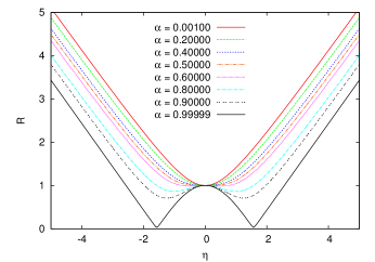
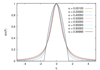
Figure 1: Plots of (a) the metric function $R$ and (b) the chiral function $\sin F$ for several values of $\alpha$ for non-linear sigma model wormholes.

We first consider wormholes in the absence of the Skyrme term, i.e. we take the limit $1/e^{2}\to 0$. In this case the set of Einstein and matter equations is invariant under the scalings $\eta\to\lambda\eta$ and $R\to\lambda R$. In order to fix the scale we choose $r_{0}=1$. This leaves only $\alpha$ as a free parameter.

Observe that Eq. (18) reduces to $R^{2}A^{\prime}=const$. However, for symmetric solutions $A^{\prime}(0)=0$. Thus this constant has to vanish. Consequently, $A=1$ is the only solution which satisfies the boundary condition $A(\eta\to\infty)\to 1$, which implies that the mass vanishes.

We have solved the coupled set of Einstein-matter equations numerically for $0\leq\alpha<1$. As examples we show in Fig. 1 the functions $R(\eta)$ and $\sin F(\eta)$ for several values of $\alpha$. In Fig. 1 we see that the areal radius $R$ possesses a minimum at $\eta=0$ when $\alpha\leq\alpha_{\rm cr}=1/2$. These solutions possess a single throat. For larger values of $\alpha$, however, $R$ possesses a local maximum at $\eta=0$ and two minima located symmetrically to each side of the local maximum. Consequently, these wormholes possess a double throat. As $\alpha$ is increased the minima become more pronounced. Thus the size of the two throats shrinks and tends to zero as $\alpha$ tends to the value one. In this limit the locations of the throats are at the values $\pm\pi/2$. The behaviour of the chiral profile function is demonstrated in Fig. 1 where we plot $\sin F$ as a function of $\eta$. Note that the function becomes more and more concentrated on the interval $-\pi/2\leq\eta\leq\pi/2$ as $\alpha$ approaches one.

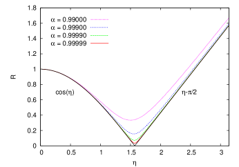
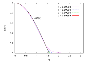
Figure 2: Same as Fig. 1 but for values of $\alpha$ close to the limit $\alpha=1$.

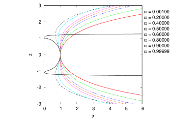
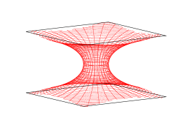
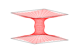
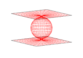
Figure 3: (a) The isometric embedding of NLS model wormholes is shown for several values of $\alpha=0$. (b-d) Three dimensional view of the isometric embedding for (b) $\alpha=0.001$, (c) $\alpha=0.8$ and (d) $\alpha=0.99999$.

The limit $\alpha\to 1$ is demonstrated in Fig. 2. We conclude that the limiting solution consists of three parts. On the interval $-\pi/2<\eta<\pi/2$ the areal radius and the chiral profile function are

$$R(\eta)=\cos\eta\ ,\ \ \ \ F(\eta)=\frac{\pi}{2}-\eta\ .$$ (25)

In this region the metric reads

$$ds^{2}=-dt^{2}+d\eta^{2}+\cos^{2}\eta\,d\Omega_{2}^{2}=-dt^{2}+d\Omega_{3}^{2}\ ,$$ (26)

and describes an Einstein universe, ${\cal M}_{E}=R_{t}\times S^{3}$. The chiral matrix $U$ is a one-to-one mapping of the three sphere $S^{3}$ to $SU(2)\sim S^{3}$. It can be easily checked that the system  (25) together with $A=1$ is indeed an exact solution of the Einstein-matter equations on the interval $-\pi/2<\eta<\pi/2$ Lechner:2000bw . Moreover, the scalar charge $D$ vanishes for this solution as can be seen from Eq. (19). This implies that there is no exotic matter present.

In the outer regions the solution reads

$$R(\eta)=\ \ \eta-\frac{\pi}{2}\ ,\ \ \ \ F(\eta)=0\ \ \ (\eta>\frac{\pi}{2}),$$ (27)

$$R(\eta)=-\eta+\frac{\pi}{2}\ ,\ \ \ \ F(\eta)=\pi\ \ \ (\eta<-\frac{\pi}{2}).$$ (28)

In both regions the metric describes the Minkowski space-time,

$$ds^{2}=-dt^{2}+dR^{2}+R^{2}d\Omega_{2}^{2}\ ,$$ (29)

and the chiral matrix $U$ is the trivial map $U=\pm 1$. Also in these regions the scalar charge vanishes, as it should for a vacuum solution.

The resulting space-time consists of two distinct Minkowski space-times plus one Einstein universe. The origin of one of the Minkowski space-times is identified with the north pole of the spatial $S^{3}$ of the Einstein universe, and the origin of the other Minkowski space-time is identified with the south pole of the $S^{3}$.

Note, that at the “glueing points” (i.e. $\eta=\pm\pi/2$) the derivative of the function $R$ and the profile function $F$ possess jump discontinuities which lead to $\delta$-function terms in the second derivatives. However, the metric depends on the function $R^{2}$, which has a discontinuity only in the fourth derivative. Hence the Ricci tensor and the Kretschmann scalar possess discontinuities at $\eta=\pm\pi/2$, but no $\delta$-function terms .

The geometry of a spatial hyper-surface of the wormhole space-times is visualized in Fig. 3. Here we show examples of the isometric embedding of the equatorial plane $\theta=\pi/2$ for several values of $\alpha$. The embedding is given by the parametric representation

$$\rho(\eta)=R(\eta)\ ,\ \ \ \ z(\eta)=\int_{0}^{\eta}\sqrt{1-R^{\prime 2}}\ d\eta^{\prime}\ .$$ (30)

We observe that the radius $R$ has a single minimum at $z=0$ if $\alpha<\alpha_{\rm cr}$, corresponding to the waist in Fig. 3. The minimum becomes degenerate if $\alpha=\alpha_{\rm cr}$ and turns to a (local) maximum for larger values of $\alpha$, corresponding to the belly in Fig. 3. Close to the limit $\alpha\to 1$ the outer regions are represented by the two plains whereas the inner region forms a sphere, as shown in Fig. 3.

IV.2 Skyrmionic Wormholes

We now turn to wormholes in the presence of the Skyrme term. In this case the coupling parameter $e$ can be included in the scaled quantities by letting

$$\eta=\frac{\tilde{\eta}}{e\kappa}\ ,\ \ \ R=\frac{\tilde{R}}{e\kappa}\ ,\ \ \ \phi=\kappa\tilde{\phi}\ ,\ \ \ 4\pi G=\frac{\alpha}{\kappa^{2}}\ ,\ \ \ D=\tilde{D}e\ ,$$ (31)

or, equivalently, by setting $e=1$.

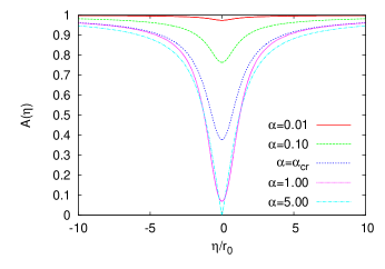
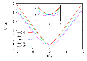
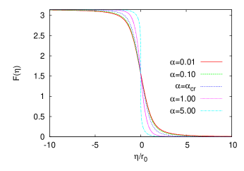
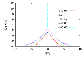
Figure 4: Plots of (a) the metric function $A$, (b) the function $R$, (c) the chiral profile function $F$ and (d) the Kretschmann scalar $K$ are presented for Skyrmionic wormholes when $r_{0}=1$, $\alpha=0.01$, $0.1$ and $\alpha_{\rm cr}=1/3$, $1.0$, $5.0$.

If the Skyrme term is present, the corresponding Einstein-matter equations are no longer scale-invariant. Then $r_{0}$ and $\alpha$ can be considered as free parameters. In Fig. 4 we show examples of solutions for $r_{0}=1$ for different values of $\alpha$. We observe that in the limit of vanishing $\alpha$ the metric functions approach the massless Ellis solution, that is, $A(\eta)=1$ and $R^{2}(\eta)=\eta^{2}+r_{0}^{2}$. Thus, we obtain a Skyrmion in the background of the Ellis wormhole space-time in this limit. As $\alpha$ is increased from zero the metric functions deviate from the Ellis solution. From Fig. 4 we see that when $\alpha$ exceeds a critical value, the minimum of the areal radius splits into two minima separated by a local maximum. Thus again the single throat splits into a double throat and an equator inbetween. As $\alpha$ becomes large the metric function $A$ tends to zero at the equator, while the Kretschmann scalar tends to diverge at the equator.

In Figs. 5 and 5 plots of the scaled mass $\mu/\alpha=M/M_{0}$ with $M_{0}=4\pi\kappa/e$ and the scaled scalar charge $\sqrt{\alpha}D$ are presented versus $r_{0}$ for different values of the parameter $\alpha$. We observe that for $\alpha\leq 1$ solutions exist for arbitrarily large values of $r_{0}$. In order to identify the limit $r_{0}\to\infty$ we introduce the scaled coordinate $\hat{\eta}=\eta/r_{0}$ and the scaled function $\hat{R}=R/r_{0}$. From the Einstein equations (17), (18) and the chiral equation (13) it follows that in the limit $r_{0}\to\infty$ all terms resulting from the Skyrme term are suppressed as $1/r_{0}^{2}$ and will vanish. However, this is exactly the limit $1/e^{2}\to 0$ discussed in the previous section. Thus, the Skyrmionic wormholes approach the NLS model wormholes (after rescaling) when $r_{0}$ becomes very large, provided that $\alpha\leq 1$.

Let us now consider the case $\alpha>1$. In this case, NLS wormholes do not exist any more and we expect a different scenario. Indeed, we see from Figs. 5 and 5 that Skyrmionic wormholes exist only up to a maximal value $r_{0,\rm max}$, which depends on $\alpha$. The mass and the scalar charge tend to zero when $r_{0}$ tends to $r_{0,\rm max}$.

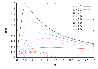
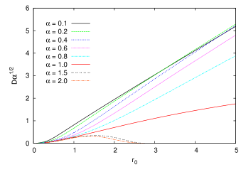
Figure 5: Plots of (a) the scaled mass $\mu/\alpha$ and (b) the scaled scalar charge $D\sqrt{\alpha}$ are shown for Skyrmionic wormholes as functions of $r_{0}$ for different values of $\alpha$.

In Fig. 6 we demonstrate that in the limit $r_{0}\to r_{0,\rm max}$ the solutions become singular. In particular, Fig. 6 displays the function $R$ when $\alpha=1.5$ for several values of $r_{0}$ approaching the maximal value $r_{0,\rm max}$. We see that the minimum of $R$ approaches zero at the points $\pm\eta_{0}$. In Fig. 6 it is seen that the Kretschmann scalar diverges at $\pm\eta_{0}$ when $r_{0}$ tends to the maximal value $r_{0,\rm max}$.

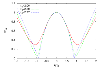
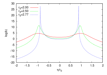
Figure 6: Plots of (a) the function $R$ and (b) the Kretschmann scalar $K$ for Skyrmionic wormholes when $\alpha=1.5$ for different values of $r_{0}$ close to the maximal value $r_{0,\rm max}$.

The geometry of a spatial hyper-surface of the wormhole space-times is visualized in Fig. 7. Here the isometric embedding of the equatorial plane $\theta=\pi/2$ for wormholes is presented when $r_{0}=1$ for several values of $\alpha$ (as examples). We observe that the radius $R$ has a single minimum at $z=0$ if $\alpha<\alpha_{\rm cr}$, corresponding to the waist in Fig. 7. The minimum becomes degenerate at $\alpha=\alpha_{\rm cr}$ and turns into a (local) maximum for larger values of $\alpha$, corresponding to the belly presented in Fig. 7.

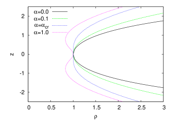
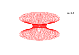
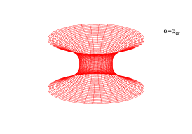
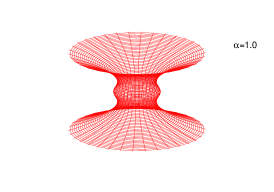
Figure 7: (a) The isometric embedding of Skyrmionic wormholes is presented when $r_{0}=1$ while $\alpha=0$ (Ellis), $\alpha=0.1$, $\alpha=\alpha_{\rm cr}$ and $\alpha=1.0$. (b-d) Three dimensional view of the isometric embedding of the wormholes when $r_{0}=1$ while (b) $\alpha=0.1$, (c) $\alpha=\alpha_{\rm cr}$ and (d) $\alpha=1.0$.

Incidentally, we have also obtained Skyrmionic wormholes with higher topological charge, but not yet performed a systematic study of them.

V Stability Analysis

The stability of wormholes is crucial for their physical relevance. Recently, it was shown that the Ellis wormhole possesses an unstable mode Gonzalez:2008wd ; Bronnikov:2011if . The unstable mode was missed before because the gauge condition had been taken too stringent. Here we do not follow the approach of Gonzalez:2008wd ; Bronnikov:2011if , since this would require the metric in closed form. Instead, we make a careful choice of the gauge condition, which ensures that we do not miss the unstable mode present in the Ellis wormhole. In fact we find that all our chiral wormholes are unstable.

We restrict to a linear stability analysis in the spherically symmetric sector. Our starting point is the spherically symmetric metric in the general form

$$ds^{2}=-e^{2\nu(t,\eta)}e^{\lambda(t,\eta)}dt^{2}+e^{-\lambda(t,\eta)}d\eta^{2}+e^{\sigma(t,\eta)}d\Omega_{2}^{2}\ ,$$ (32)

and the time-dependent Ansätze for the chiral matrix and the phantom field

$$U=\cos F(t,\eta)+i\sin F(t,\eta)\ \vec{e}\cdot\vec{\tau}\ ,\ {\rm resp.}\ \ \phi=\phi(t,\eta)\ .$$ (33)

We derive the Einstein-matter equations for these Ansätze and consider the perturbed metric, scalar field and chiral profile functions

$$\nu(\eta,t) = \bar{\nu}(\eta)+\delta\nu(\eta)e^{i\omega t},$$

$$\lambda(\eta,t) = \bar{\lambda}(\eta)+\delta\lambda(\eta)e^{i\omega t},$$

$$\sigma(\eta,t) = \bar{\sigma}(\eta)+2\delta\sigma(\eta)e^{i\omega t},$$

$$\phi(\eta,t) = \bar{\phi}(\eta)+\delta\phi(\eta)e^{i\omega t},$$

$$F(\eta,t) = \bar{F}(\eta)+\delta F(\eta)e^{i\omega t}.$$

Here $\bar{F}$ and $\bar{\phi}$ denote the unperturbed chiral and phantom field functions, respectively, whereas the unperturbed metric functions obey

$$e^{\bar{\nu}}=A,\ \ \ e^{\bar{\lambda}}=1,\ \ \ e^{\bar{\sigma}}=R^{2}\ .$$

Next we expand the Einstein-matter equations up to first order in the small quantities $\delta\nu(\eta)$, $\delta\lambda(\eta)$, $\delta\sigma(\eta)$, $\delta\phi(\eta)$ and $\delta F(\eta)$. The resulting set of linear ODEs for the perturbations form an eigenvalue problem with eigenvalue $\omega^{2}$. If $\omega^{2}$ is negative the perturbations increase in time, indicating that the solution is unstable.

We can use the gauge freedom to reduce the number of linear ODEs. Consider the ODE for the perturbation of the phantom field

$$\left[\frac{R^{2}}{A}\left(\delta\phi^{\prime}+\bar{\phi}^{\prime}\left(2\delta\sigma+\delta\lambda+\delta\nu\right)\right)\right]^{\prime}+\omega^{2}\frac{R^{2}}{A}\delta\phi=0\ .$$ (34)

This form suggests the gauge condition newpap

$$\delta\nu+\delta\lambda+2\delta\sigma=0\ .$$ (35)

Moreover, we argue that, with (35), the function $\delta\phi$ vanishes identically, if there exists an unstable mode, i.e. if $\omega^{2}$ is negative. Indeed, taking the gauge condition Eq. (35) into account we multiply Eq. (34) by $\delta\phi$ and integrate over $(-\infty,\infty)$. This yields after integration by parts

$$\left.\left(\frac{R^{2}}{A}\delta\phi\delta\phi^{\prime}\right)\right|_{-\infty}^{\infty}=\int_{-\infty}^{\infty}\left[\frac{R^{2}}{A}\left({\delta\phi^{\prime}}^{2}-\omega^{2}\delta\phi^{2}\right)\right]d\eta\ .$$

Since the left-hand-side of this equation vanishes for normalizable $\delta\phi$, the integral on the right-hand-side also vanishes. However, for negative $\omega^{2}$ the integrand is positive. Therefore, the integral can only vanish if $\delta\phi$ is identically zero.

With $\delta\phi=0$ and $\delta\nu=-\delta\lambda-2\delta\sigma$ the resulting equations consist of three second order ODEs for the functions $\delta\sigma$, $\delta\lambda$ and $\delta F$ in addition to the constraint

$$R^{\prime}\delta\lambda+2A\left[\frac{R}{A}\delta\sigma\right]^{\prime}+2\alpha\frac{\bar{F}^{\prime}\delta F}{R}\left(\frac{2\sin^{2}F}{e^{2}}+R^{2}\right)=0\ .$$ (36)

In principle, the constraint for the function $\delta\lambda$ can be solved in order to reduce the three second order ODEs to only two for the corresponding functions $\delta\sigma$ and $\delta F$. However, this would introduce factors $1/R^{\prime}$ in the ODEs, which diverge when $R$ becomes extremal. Therefore, we choose to solve the system of the three ODEs numerically and just verify that the constraint Eq. (36) is satisfied.

The boundary conditions follow from the requirement that the perturbations have to vanish in the asymptotic regions, that is,

$$\delta\sigma(\pm\infty)=\delta\lambda(\pm\infty)=\delta F(\pm\infty)=0\ .$$ (37)

In addition, in order to ensure that the perturbations are normalizable we impose the condition $\sigma(0)=1$. The eigenvalue $\omega^{2}$ has to be adjusted such that the perturbations satisfy the asymptotic boundary conditions .

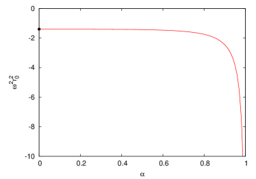
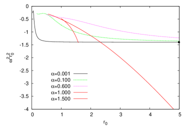
Figure 8: Plots of (a) the scaled eigenvalue for the NLS wormholes as a function of $\alpha$ and (b) the scaled eigenvalue for the Skyrmionic wormholes as a function of $r_{0}$ for different values of $\alpha$. The dot in (a) and (b) indicates the eigenvalue of the Ellis wormhole.

The numerical results are demonstrated in Fig. 8. The case of the NLS wormholes is displayed in Fig. 8, where the eigenvalue is shown as a function of $\alpha$. Here the dot indicates the eigenvalue of the Ellis wormhole Gonzalez:2008wd . We observe that $\omega^{2}$ is negative and decreases with increasing $\alpha$. Thus we conclude that all NLS wormholes are unstable. In Fig. 8 the stability analysis of the Skyrmionic wormholes is summarized. In particular, the eigenvalue as a function of $r_{0}$ for several values of $\alpha$ is shown. As in the case of NLS wormholes, we conclude that $\omega^{2}$ is negative for all solutions. Hence the Skyrmionic wormholes are unstable as well.

VI Non-symmetric Skyrmionic Wormhole Solutions

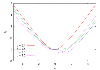
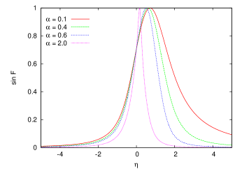
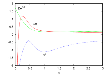
Figure 9: Plots of (a) the areal radius $R(\eta)$, (b) the function $\sin F(\eta)$, and (c) the dimensional mass $\mu/\alpha$ and scalar charge $D/\sqrt{\alpha}$ as well as the unstable mode for the non-symmetric Skrymionic wormholes for different values of $\alpha$ when $r_{0}=1$ and $F_{0}=3\pi/4$.

The wormholes we considered so far possess the symmetry $A(-\eta)=A(\eta)$, $R(-\eta)=R(\eta)$ and $F(-\eta)=\pi-F(\eta)$. The last property implies $F(0)=\pi/2$. However, since $F(0)=F_{0}$ is a free parameter we can choose $F_{0}\neq\pi/2$. Such a choice breaks the symmetry with respect to $\eta\to-\eta$ and leads to non-symmetric wormholes. As an example we consider the non-symmetric Skyrmionic wormholes for fixed parameters $F_{0}=3\pi/4$ and $r_{0}=1$ and varying coupling parameter $\alpha$. The areal radius $R$ and the function $\sin F$ are shown for several values of $\alpha$ in Figs. 9 and 9, respectively. As can be seen from Fig. 9, the asymmetry of the areal function $R$ is larger for large $\alpha$. In contrast, Fig.  9 shows that the asymmetry of the chiral field is more pronounced for small values of $\alpha$. However, one should keep in mind that $\alpha$ is the coupling strength in the Einstein equations. Thus, for small $\alpha$ the asymmetry of the chiral field does not affect the space-time metric very much, leading to an almost symmetric function $R$. On the other hand, for large $\alpha$ the asymmetry of the chiral field has considerable effect on the metric and induces an asymmetry in the metric functions. From Fig. 9 we observe that with increasing $\alpha$ the minimum of the areal function turns to a maximum and two local minima next to it. This is similar to the symmetric solutions, however the depths of the two minima differ and they are not located symmetrically around the maximum. These non-symmetric wormhole solutions thus also possess two non-symmetric throats.

Fig. 9 displays the scaled mass parameter $\mu/\alpha$ and the scaled scalar charge $D\sqrt{\alpha}$ in terms of $\alpha$. We observe that $\mu/\alpha$ assumes negative values for small $\alpha$, possesses a maximum at $\alpha\approx 0.26$, and tends to some finite value for large $\alpha$. In addition, Fig.9 displays the eigenvalue $\omega^{2}$ of the unstable mode. Since $\omega^{2}$ is negative we conclude that the non-symmetric Skyrmionic wormholes (as considered so far) are, also, unstable.

VII Conclusion

We have considered Morris-Thorne wormholes threaded by chiral fields that carry a conserved topological charge. We have focussed on static spherically symmetric solutions, which are symmetric under an interchange of the two asymptotically flat universes with respect to the throat.

When the chiral fields are described by the NLS model, the coupling parameter $\alpha$ is the single free parameter for symmetric wormholes. For small $\alpha$ the chiral fields have hardly any influence upon the wormhole geometry, and the solutions possess a single throat. As the coupling parameter increases, the presence of the chiral fields starts to be felt by the geometry. At a critical coupling $\alpha_{\rm cr}$, the throat becomes degenerate. Beyond $\alpha_{\rm cr}$ the wormhole then exhibits a set of three extrema, a (local) maximal surface and two minimal surfaces located symmetrically, one on each side. Thus the wormhole possesses a double throat with a belly in the interior.

As $\alpha$ increases further the chiral fields become more and more localized in the inner region of the belly. At the maximal coupling $\alpha_{\rm max}$ finally, the chiral fields are fully localized inside this inner region, while the areal radius of the two throats decreases to zero. The space-time then splits into three parts. The outer parts correspond to empty Minkowski spaces, while the inner part corresponds to an Einstein universe with a chiral field carrying topological charge one.

In the presence of a Skyrme term, we have one more free parameter. Thus we can vary the gravitational coupling and the throat size independently. With increasing $\alpha$ we again observe an increasing influence of the matter on the geometry of the throat, and the formation of two throats with an inner belly beyond a critical value $\alpha_{\rm cr}$. The splitting of the space-time into three parts is, however, less smooth than in the NLS case.

By choosing the boundary conditions asymmetrically with respect to the throat we can distribute the chiral fields asymmetrically with respect to the two asymptotically flat universes. Then the deformation of the wormhole by the matter is asymmetric as well. Consequently, when the single throat splits into a double throat at a critical coupling, the two throats develop asymmetrically with respect to their location and size. This may possibly lead to only a single throat reaching zero, resulting in a breakup of the space-time into only two parts at a maximal coupling.

Let us now think of the Skyrmionic wormholes as Skyrmions passing a wormhole. Clearly, one would have to make time-dependent calculations to model such a transit. However, the static calculations may already give us some hints of what to expect. In particular, we conclude that the Skyrmions will deform the wormhole geometry and possibly even let the space-time pinch, resulting in two or three disconnected parts.

Let us conclude by stating that the chiral fields cannot stabilize the wormhole space-time. The instability of the Ellis solution is inherited by the wormholes threaded by chiral fields, although they do carry a topological charge. According to our observations this is not surprising though, since the topological charge may finally simply reside in a single of several disconnected space-time parts.

References

- (1) For an overview see e. g. M. Visser, “Lorentzian wormholes: From Einstein to Hawking”, Woodbury, USA: AIP (1995) 412 p
- (2) A. Einstein and N. Rosen, Phys. Rev. 48 (1935) 73.
- (3) J. A. Wheeler, Annals Phys. 2, 604-614 (1957).
- (4) J. A. Wheeler, Geometrodynamics (Academic, New York, 1962).
- (5) M. D. Kruskal, Phys. Rev. 119, 1743-1745 (1960).
- (6) R. W. Fuller, J. A. Wheeler, Phys. Rev. 128, 919-929 (1962).
- (7) I. H. Redmount, Prog. Theor. Phys. 73 (1985) 140.
- (8) D. M. Eardley, Phys. Rev. Lett. 33, 442-444 (1974).
- (9) R. M. Wald, S. Ramaswamy, Phys. Rev. D21, 2736-2741 (1980).
- (10) M. S. Morris, K. S. Thorne, Am. J. Phys. 56, 395-412 (1988).
- (11) H. G. Ellis, J. Math. Phys. 14, 104-118 (1973).
- (12) H. G. Ellis, Gen. Rel. Grav. 10, 105-123 (1979).
- (13) K. A. Bronnikov, Acta Phys. Polon. B4, 251-266 (1973).
- (14) T. Kodama, Phys. Rev. D18, 3529-3534 (1978).
- (15) C. Armendariz-Picon, Phys. Rev. D65, 104010 (2002) [gr-qc/0201027].
- (16) V. Dzhunushaliev, V. Folomeev, B. Kleihaus and J. Kunz, JCAP 1104, 031 (2011) [arXiv:1102.4454 [astro-ph.GA]].
- (17) V. Dzhunushaliev, V. Folomeev, B. Kleihaus and J. Kunz, Phys. Rev. D 85, 124028 (2012) [arXiv:1203.3615 [gr-qc]].
- (18) V. Dzhunushaliev, V. Folomeev, B. Kleihaus and J. Kunz, “Mixed neutron-star-plus-wormhole systems: Linear stability analysis”, [arXiv:1302.5217 [gr-qc]].
- (19) D. Hochberg, Phys. Lett. B251, 349-354 (1990).
- (20) H. Fukutaka, K. Tanaka, K. Ghoroku, Phys. Lett. B222, 191-194 (1989).
- (21) K. Ghoroku, T. Soma, Phys. Rev. D46, 1507-1516 (1992).
- (22) N. Furey, A. DeBenedictis, Class. Quant. Grav. 22, 313-322 (2005). [gr-qc/0410088].
- (23) K. A. Bronnikov and E. Elizalde, Phys. Rev. D 81, 044032 (2010) [arXiv:0910.3929 [hep-th]].
- (24) P. Kanti, B. Kleihaus and J. Kunz, Phys. Rev. Lett. 107, 271101 (2011) [arXiv:1108.3003 [gr-qc]].
- (25) P. Kanti, B. Kleihaus and J. Kunz, Phys. Rev. D 85 (2012) 044007 [arXiv:1111.4049 [hep-th]].
-
(26)
H. Luckock and I. Moss,
Phys. Lett. B176 (1986) 341;
H. Luckock, Black hole skyrmions, Proceedings of the 1986 Paris-Meudon Colloquium, eds. H. J. de Vega, and N. Sanchez, (World Scientific, Singapore, 1987). - (27) S. Droz, M. Heusler and N. Straumann, Phys. Lett. B 268, 371 (1991).
- (28) J. A. Gonzalez, F. S. Guzman and O. Sarbach, Class. Quant. Grav. 26 (2009) 015010 [arXiv:0806.0608 [gr-qc]].
- (29) K. A. Bronnikov, J. C. Fabris and A. Zhidenko, Eur. Phys. J. C 71 (2011) 1791 [arXiv:1109.6576 [gr-qc]].
- (30) M. Heusler, S. Droz and N. Straumann, Phys. Lett. B 271, 61 (1991).
- (31) M. Heusler, S. Droz and N. Straumann, Phys. Lett. B 285, 21 (1992).
- (32) This solution has been discussed before in C. Lechner, S. Husa and P. C. Aichelburg, Phys. Rev. D 62 (2000) 044047 [gr-qc/0002031].