Characterization of worst-case GMRES

Abstract

Given a matrix $A$ and iteration step $k$, we study a best possible attainable upper bound on the GMRES residual norm that does not depend on the initial vector $b$. This quantity is called the worst-case GMRES approximation. We show that the worst case behavior of GMRES for the matrices $A$ and $A^{T}$ is the same, and we analyze properties of initial vectors for which the worst-case residual norm is attained. In particular, we show that such vectors satisfy a certain “cross equality”, and we characterize them as right singular vectors of the corresponding GMRES residual matrix. We show that the worst-case GMRES polynomial may not be uniquely determined, and we consider the relation between the worst-case and the ideal GMRES approximations, giving new examples in which the inequality between the two quantities is sharp at all iteration steps $k\geq 3$. Finally, we give a complete characterization of how the values of the approximation problems in the context of worst-case and ideal GMRES for a real matrix change, when one considers complex (rather than real) polynomials and initial vectors in these problems.

1 Introduction

Let a nonsingular matrix $A\in\mathbb{R}^{n\times n}$ and a vector $b\in\mathbb{R}^{n}$ be given. Consider solving the system of linear algebraic equations $Ax=b$ with the initial guess $x_{0}=0$ using the GMRES method [11]. This method generates a sequence of iterates $x_{k}\in\mathcal{K}_{k}(A,b)\equiv{\rm span}\{b,Ab,\dots A^{k-1}b\}$, $k=1,2,\dots\,$, so that the corresponding $k$th residual $r_{k}\equiv b-Ax_{k}$ satisfies

$$\|r_{k}\|\;=\;\min_{p\in\pi_{k}}\,\|\,p(A)b\,\|\,.$$ (1)

Here $\|\cdot\|$ denotes the Euclidean norm, and $\pi_{k}$ denotes the set of real polynomials of degree at most $k$ and with value one at the origin. Note that for a real matrix $A$ and a real right hand side $b$ the minimum in (1) is achieved for a real polynomial. Considering only real polynomials therefore does not represent any restriction.

It is clear from (1), that the sequence of GMRES residual norms $\|r_{k}\|$, $k=1,2,\dots\,,$ is nonincreasing. It terminates with $r_{k}=0$ if and only if $k$ is equal to $d(A,b)$, the degree of the minimal polynomial of the vector $b$ with respect to $A$. For each $b$ we have $d(A,b)\leq d(A)$, the degree of the minimal polynomial of $A$.

A geometric characterization of the iterate $x_{k}\in\mathcal{K}_{k}(A,b)$, which is mathematically equivalent to (1), is given by

$$r_{k}\;\perp\;A\mathcal{K}_{k}(A,b)\,.$$ (2)

To emphasize the dependence of the $k$th GMRES residual $r_{k}$ on the given data $A$, $b$ and $k$ we will sometimes write

$$r_{k}=\mathrm{GMRES}(A,b,k)\qquad\mbox{or}\qquad r_{k}=p_{k}(A)b,$$

where $p_{k}\in\pi_{k}$ is the $k$th GMRES polynomial of $A$ and $b$, i.e., the polynomial that solves the minimization problem on the right hand side of (1). As long as $r_{k}\neq 0$, this polynomial is uniquely determined. The matrix $p_{k}(A)$ is called the $k$th GMRES residual matrix of $A$ and $b$. For further basic properties and algorithmic details of the GMRES method we refer to the original paper [11] or the books [2, 8, 10].

In the following we will assume without loss of generality that $\|b\|=1$. A common approach for investigating the GMRES convergence behavior is to bound (1) independently of $b$. For each iteration step $k$ the best possible bound on the GMRES residual norm that is independent of $b$ is given by maximizing the right hand side of (1) over all unit norm vectors, i.e.,

$$\|r_{k}\|\;=\;\min_{p\in\pi_{k}}\,\|\,p(A)b\,\|\;\leq\;\max_{\|v\|=1}\min_{p\in\pi_{k}}\|\,p(A)v\,\|\;\equiv\;\Psi_{k}(A)\,.$$ (3)

The quantity $\Psi_{k}(A)$ is called the $k$th worst-case GMRES approximation. It is easy to see that the bound (3) is sharp in the sense that for each given $A$ and $k$ there exists a unit norm vector $b$ so that the corresponding $k$th GMRES residual vector satisfies $\|r_{k}\|=\Psi_{k}(A)$. We will call such a vector $b$, the corresponding $k$th GMRES polynomial $p_{k}$ and the corresponding $k$th GMRES residual matrix $p_{k}(A)$ the $k$th worst-case GMRES initial vector, polynomial and residual matrix, respectively. If $A$ is singular, then $\Psi_{k}(A)=1$ for all $k\geq 0$ (to see this, simply take $b$ as a unit norm vector in the kernel of $A$). Hence only the case of a nonsingular matrix $A$ is of interest in this context. For such $A$ we have

$$1\geq\Psi_{1}(A)\geq\cdots\geq\Psi_{d(A)-1}(A)>\Psi_{d(A)}(A)=0,$$

and therefore we only need to consider $1\leq k\leq d(A)-1$.

It is known that $\Psi_{k}(A)$ for a fixed $k$ is a continuous function on the open set of nonsingular matrices; see [5, Theorem 3.1] or [1, Theorem 2.5]. Moreover, it was shown in [1, Theorem 2.7] that $\Psi_{k}(A)=1$ for a nonsingular matrix $A$, if and only if zero is contained in some generalized field of values derived from the powers $I,A,\dots,A^{k}$. Most of the other previously published results on worst-case GMRES are devoted to studying the tightness of the inequality

$$\Psi_{k}(A)\;\leq\;\min_{p\in\pi_{k}}\|p(A)\|\;\equiv\varphi_{k}(A),$$ (4)

which is easily derived from (3) using the submultiplicativity property of the Euclidean norm. The quantity $\varphi_{k}(A)$ is called the $k$th ideal GMRES approximation [4]. The polynomial for which the minimum is attained in (4) is called the $k$th ideal GMRES polynomial of $A$. This polynomial is uniquely determined; see [4, 9]. It was shown that (4) is an equality for normal matrices $A$ and all $k\geq 0$, and for $k=1$ and any nonsingular $A$ [3, 6]. Some nonnormal matrices $A$ are known for which $\Psi_{k}(A)<\varphi_{k}(A)$, even $\Psi_{k}(A)\ll\varphi_{k}(A)$, for certain $k$; see [1, 13].

The ideal GMRES approximation problem can be formulated as a semidefinite program (see [14]) and hence can be solved efficiently by standard software. On the other hand, we are unaware of any efficient algorithm for solving the worst-case GMRES approximation problem, so that in practice one needs to resort to a “general purpose” nonlinear solver to compute worst-case GMRES data. The difficult nonlinear nature of the worst-case GMRES approximation problem may be one of the reasons why this problem is less studied (both theoretically and numerically) than the ideal GMRES approximation problem.

This paper is mainly devoted to characterizations of the worst-case GMRES problem (3). We first show in Section 2 that $\Psi_{k}(A)=\Psi_{k}(A^{T})$, and that worst-case initial vectors satisfy a certain “cross equality”. Next, in Section 3, we look at the worst-case GMRES approximation problem from the optimization point of view and show that $k$th worst-case GMRES initial vectors are always right singular vectors of the corresponding $k$th GMRES residual matrix. In Section 4 we prove that a $k$th worst-case GMRES polynomial may not be uniquely determined (unlike the $k$th ideal GMRES polynomial), and we give a numerical example for two different polynomials and corresponding initial vectors that both attain the same worst-case GMRES value at the same step $k$. In Section 5 we further study differences between the worst-case and the ideal GMRES approximations. In particular, we state a parameterized set of matrices $A$ of arbitrary size $2n$ (with $n\geq 2$) for which the inequality in (4) is sharp for all $k=3,\dots,2n-1$. In the previously published examples in [1, 13], a small matrix $A$ is constructed for which the sharp inequality occurs for exactly one $k$. Finally, in Section 6 we analyze whether the values of the max-min approximation (3) and the min-max approximation (4) for a real matrix change if we consider the maximization over complex vectors and/or the minimization over complex polynomials. This analysis gives another indication for the difference between the two approximation problems.

2 The cross equality

In this section we generalize two results of Zavorin [15]. The first shows that $\Psi_{k}(A)=\Psi_{k}(A^{T})$ and the second concerns a special property of worst-case initial vectors (they satisfy the so-called “cross equality”). Note that Zavorin proved these results only for diagonalizable matrices using quite a complicated technique based on the decomposition of the corresponding Krylov matrix. Using a simple algebraic technique we prove these results for general matrices. All results presented in this section can easily be generalized from real to complex matrices.

Theorem 1.

If $A\in\mathbb{R}^{n\times n}$ is a nonsingular matrix, then $\Psi_{k}(A)=\Psi_{k}(A^{T})$ for all $k=1,\dots,d(A)-1$.

Proof.

Let $1\leq k\leq d(A)-1$ and consider any unit norm vector $b$ such that the corresponding $k$th GMRES residual vector $r_{k}=p_{k}(A)b$ is nonzero. The defining property (2) of $r_{k}$ means that $\langle A^{j}b,r_{k}\rangle=0$ for $j=1,\dots,k$. Hence, for any $q\in\pi_{k}$,

$$\|r_{k}\|^{2}=\langle p_{k}(A)b,r_{k}\rangle=\langle b,r_{k}\rangle=\langle q(A)b,r_{k}\rangle=\langle b,q(A^{T})r_{k}\rangle\leq\|q(A^{T})r_{k}\|,$$ (5)

where the last inequality follows from the Cauchy-Schwarz inequality and $\|b\|=1$.

If $b$ is a unit norm $k$th worst-case GMRES initial vector and $r_{k}$ is the corresponding $k$th GMRES residual vector, then the previous inequality means that

$$\|r_{k}\|^{2}\;=\;\Psi_{k}^{2}(A)\;\leq\;\|q(A^{T})r_{k}\|,$$ (6)

where $q\in\pi_{k}$ is arbitrary. Dividing by $\|r_{k}\|$ and taking the minimum over all $q\in\pi_{k}$ we get

$$\Psi_{k}(A)\leq\min_{q\in\pi_{k}}\left\|q(A^{T})\frac{r_{k}}{\|r_{k}\|}\right\|\leq\Psi_{k}(A^{T}).$$ (7)

Now we can reverse the roles of $A$ and $A^{T}$, and then repeat the whole argument to obtain the opposite inequality, i.e., $\Psi_{k}(A^{T})\leq\Psi_{k}(A)$. ∎

The following theorem describes a special property of worst-case initial vectors: If we apply GMRES to $A$ and a unit norm $k$th worst-case initial vector $b$ giving at step $k$ the residual vector $r_{k}$, and then $k$ steps of GMRES to $A^{T}$ and the initial vector $r_{k}/\|r_{k}\|$, we obtain again the original initial vector $b$ (up to a scaling factor).

Theorem 2.

Let $A\in\mathbb{R}^{n\times n}$ be a nonsingular matrix, and let $1\leq k\leq d(A)-1$. If $b\in\mathbb{R}^{n}$ is a unit norm $k$th worst-case GMRES initial vector and

$$r_{k}\equiv\mathrm{GMRES}(A,b,k),\qquad s_{k}\equiv\mathrm{GMRES}\left(A^{T},\frac{r_{k}}{\|r_{k}\|},k\right),$$

then

$$\|s_{k}\|=\|r_{k}\|=\Psi_{k}(A)\qquad\mbox{and}\qquad b=\frac{s_{k}}{\Psi_{k}(A)}.$$

Proof.

Let $b$ be a unit norm $k$th worst-case GMRES initial vector and let $r_{k}=\mathrm{GMRES}(A,b,k)$. In addition, let $s_{k}=\mathrm{GMRES}(A^{T},r_{k}/\|r_{k}\|,k)$ and let $q_{k}$ be the corresponding $k$th GMRES polynomial. Using this polynomial in (6) yields

$$\|r_{k}\|=\Psi_{k}(A)\;\leq\;\left\|q_{k}(A^{T})\frac{r_{k}}{\|r_{k}\|}\right\|\;=\;\|s_{k}\|\;\leq\;\Psi_{k}(A^{T}).$$

However, as shown in Theorem 1, equality holds throughout, which shows the first assertion.

Moreover, since $\|r_{k}\|=\|s_{k}\|$, the (Cauchy-Schwarz) inequality on the right of (5) is an equality for the given $b$ and $q=q_{k}$, i.e.,

$$\langle b,q_{k}(A^{T})r_{k}\rangle=\|q_{k}(A^{T})r_{k}\|.$$

Since $\|b\|=1$, this happens if and only if

$$b\;=\;\frac{q_{k}(A^{T})r_{k}}{\|q_{k}(A^{T})r_{k}\|}\;=\;\frac{q_{k}(A^{T})r_{k}}{\|r_{k}\|\|r_{k}\|}\;=\;\frac{s_{k}}{\|r_{k}\|},$$

which finishes the proof. ∎

The previous theorem shows that if $b$ is a unit norm $k$th worst-case GMRES initial vector, then (with the same notation as in the proof above)

$$\Psi_{k}(A)b\;=\;s_{k}\;=\;q_{k}(A^{T})\frac{r_{k}}{\|r_{k}\|}=q_{k}(A^{T})p_{k}(A)\frac{b}{\|r_{k}\|},$$

or, equivalently,

$$q_{k}(A^{T})p_{k}(A)\,b\;=\;\Psi_{k}^{2}(A)\,b.$$ (8)

In other words, $b$ is an eigenvector of the matrix $q_{k}(A^{T})p_{k}(A)$ with the corresponding eigenvalue $\Psi_{k}^{2}(A)$. In Corollary 11 we will show that $q_{k}=p_{k}$, i.e., that $b$ is a right singular vector of the $k$th worst-case GMRES residual matrix $p_{k}(A)$.

To further investigate vectors with the special property introduced in Theorem 2 we use the following definition.

Definition 3.

Let $A\in\mathbb{R}^{n\times n}$ be nonsingular. We say that a unit norm vector $b\in\mathbb{R}^{n}$ with $d(A,b)>k$ satisfies the cross equality for $A$ and the step $k\geq 1$, if

$$b=\frac{s_{k}}{\|s_{k}\|},\quad\mbox{where}\quad s_{k}\equiv\mathrm{GMRES}\left(A^{T},\frac{r_{k}}{\|r_{k}\|},k\right),\quad r_{k}\equiv\mathrm{GMRES}(A,b,k).$$

Algorithm 1 (Cross iterations 1)

  $b^{(0)}=b$,

  for $j=1,2,\dots$ do

     $r_{k}^{(j)}=\mathrm{GMRES}(A,b^{(j-1)},k)$

     $c^{(j-1)}=r_{k}^{(j)}/\|r_{k}^{(j)}\|$

     $s_{k}^{(j)}=\mathrm{GMRES}(A^{T},c^{(j-1)},k)$

     $b^{(j)}=s_{k}^{(j)}/\|s_{k}^{(j)}\|$

  end for

Inspired by Theorem 2 we define the iterative process shown in Algorithm 1. To analyze this algorithm, let us denote

$$r_{k}^{(j)}=p_{k}^{(j)}(A)b^{(j-1)}\quad\mbox{and}\quad s_{k}^{(j)}=q_{k}^{(j)}(A^{T})c^{(j-1)}.$$

Using $q=q_{k}^{(j)}$ in (5) we then get

$$\|r_{k}^{(j)}\|^{2}\;\leq\;\|q_{k}^{(j)}(A^{T})r_{k}^{(j)}\|\;=\;\|r_{k}^{(j)}\|\,\|q_{k}^{(j)}(A^{T})c^{(j-1)}\|\;=\;\|r_{k}^{(j)}\|\,\|s_{k}^{(j)}\|.$$

Now consider (5) with the roles of $A$ and $A^{T}$ reversed, i.e.,

$$\|s_{k}^{(j)}\|^{2} = \langle q_{k}^{(j)}(A^{T})c^{(j-1)},s_{k}^{(j)}\rangle\;=\;\langle c^{(j-1)},q(A)s_{k}^{(j)}\rangle\;=\;\|s_{k}^{(j)}\|\,\langle c^{(j-1)},q(A)b^{(j)}\rangle$$

$$\leq \|s_{k}^{(j)}\|\,\|q(A)b^{(j)}\|,$$

for all $q\in\pi_{k}$. We can choose $q=p_{k}^{(j+1)}$ and thus obtain $\|s_{k}^{(j)}\|\leq\|r_{k}^{(j+1)}\|$. In summary, we have shown that

$$\|r_{k}^{(j)}\|\leq\|s_{k}^{(j)}\|\leq\|r_{k}^{(j+1)}\|\leq\|s_{k}^{(j+1)}\|\leq\Psi_{k}(A),\quad j=1,2,\dots\,.$$ (9)

Hence the sequences of norms $\|r_{k}^{(j)}\|$ and $\|s_{k}^{(j)}\|$, $j=1,2,\dots\,$, interlace each other, are both nondecreasing, and are both bounded by $\Psi_{k}(A)$. This implies that both sequences converge to the same limit, which does not exceed $\Psi_{k}(A)$.

Consequently, for any initial vector $b^{(0)}$, Algorithm 1 converges to a vector that satisfies the cross equality for $A$ and step $k$. If $b^{(0)}$ satisfies the cross equality for $A$ and step $k$, then trivially equality holds in (9) for all $j$. On the other hand, if equality holds in (9) for one $j$, then, using (5),

$$\langle b^{(j)},q_{k}^{(j)}(A^{T})r_{k}^{(j)}\rangle=\|r_{k}^{(j)}\|^{2}=\|q_{k}^{(j)}(A^{T})r_{k}^{(j)}\|=\|s_{k}^{(j)}\|,$$

and we have reached a vector that satisfies the cross equality.

From the above it is clear that the cross equality represents a necessary condition for a vector $b^{(0)}$ to be a worst-case initial vector. On the other hand, we can ask whether this condition is sufficient, or, at least, whether the vectors that satisfy the cross equality are in some sense special. To investigate this question we present the following lemma.

Lemma 4.

Let $A\in\mathbb{R}^{n\times n}$ be nonsingular, $k\geq 1$, and $b\in\mathbb{R}^{n}$ be a unit norm initial vector with $d(A,b)>k$. If $r_{k}=\mathrm{GMRES}(A,b,k)$, then $d(A^{T},r_{k})>k$, and $b$ satisfies the cross for $A$ and the step $k$ if and only if $b\in\mathcal{K}_{k+1}(A^{T},r_{k})$. In particular, each unit norm vector $b$ with $d(A,b)=n$ satisfies the cross equality for $A$ and the step $k=n-1$.

Proof.

The nonzero GMRES residual $r_{k}\in b+A\mathcal{K}_{k}(A,b)\subset\mathcal{K}_{k+1}(A,b)$ is uniquely determined by the orthogonality conditions (2), which can be written as

$$0=\langle A^{j}b,r_{k}\rangle=\langle b,(A^{T})^{j}r_{k}\rangle,\quad\mbox{for}\quad j=1,\dots,k,$$

or, equivalently,

$$b\perp A^{T}\mathcal{K}_{k}(A^{T},r_{k}).$$ (10)

Now let $s_{k}\equiv\mbox{GMRES}(A^{T},r_{k}/\|r_{k}\|,k)$. From (5) we know that $\|s_{k}\|\geq\|r_{k}\|>0$, i.e. $d(A^{T},r_{k})>k$, and

$$s_{k}\in\frac{r_{k}}{\|r_{k}\|}+A^{T}\mathcal{K}_{k}(A^{T},r_{k})\subset\mathcal{K}_{k+1}(A^{T},r_{k}),\quad s_{k}\perp A^{T}\mathcal{K}_{k}(A^{T},r_{k})\,.$$ (11)

If $b$ satisfies the cross equality for $A$ and the step $k$, then $b=s_{k}/\|s_{k}\|$ and (11) implies that $b\in\mathcal{K}_{k+1}(A^{T},r_{k})$. On the other hand, if $b\in\mathcal{K}_{k+1}(A^{T},r_{k})$, then $\langle b,r_{k}\rangle=\|r_{k}\|^{2}\neq 0$ and (10) imply that $b=s_{k}/\|s_{k}\|$.

For $k=n-1$, we have $\mathcal{K}_{k+1}(A^{T},r_{k})=\mathbb{R}^{n}$, i.e. $b\in\mathcal{K}_{k+1}(A^{T},r_{k})$ is always satisfied. ∎

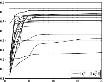
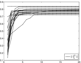
Fig. 1: Cross iterations for random initial vectors.

To give a numerical example for Algorithm 1 we consider $A$ being the Jordan block $J_{\lambda}$ of size $11$ with the eigenvalue $\lambda=1$, and we and choose $k=5$. In this case, the ideal GMRES matrix $\varphi_{5}(A)$ has a simple maximal singular value, as numerically observed in [12]. Using the results of Greenbaum and Gurvits in [3] we know that then $\Psi_{5}(J_{\lambda})=\varphi_{5}(J_{\lambda})$, and, moreover, that the corresponding worst-case initial vector is the right singular vector that corresponds to the maximal singular value of the ideal GMRES matrix $\varphi_{5}(A)$. Hence, in this case the 5th worst-case initial vector is uniquely determined up to scaling.

In the left part of Fig. 1 we show the results of Algorithm 1 started with 20 random unit norm initial vectors. Each line represents the sequence $\|r_{k}^{(j)}\|,\|s_{k}^{(j)}\|$, for $j=1,\dots,10$. In the end of each of the 20 runs we get a vector that satisfies (up to a small inaccuracy) the cross equality for $J_{\lambda}$ and $k=5$. We can observe that there are many initial vectors that satisfy the cross equality, and there seems to be no special structure in the norms that are attained in the end. In particular, none of the 20 runs results in a 5th worst-case initial vector for which the norm $\Psi_{5}(A)$ is attained (this value is visualized by the highest horizontal line in the figure).

We will now slightly modify the cross iteration Algorithm 1. Having a initial vector $b^{(j-1)}$ we always apply both, GMRES with $A$ as well as GMRES with $A^{T}$, and look at the resulting GMRES residual norm. We take as a resulting residual the one with the greater norm; see Algorithm 2. After the process converges, we get again a vector that satisfies the cross equality.

Algorithm 2 (Cross iterations 2)

  $b^{(0)}=b$,

  for $j=1,2,\dots$ do

     $v=\mathrm{GMRES}(A,b^{(j-1)},k)$

     $w=\mathrm{GMRES}(A^{T},b^{(j-1)},k)$

     if $\|v\|<\|w\|$ then

        $t_{k}^{(j)}=w$

     else

        $t_{k}^{(j)}=v$

     end if

     $b^{(j)}=t_{k}^{(j)}/\|t_{k}^{(j)}\|$

  end for

This strategy is a little better than the original one when looking for a worst-case initial vector; see Fig. 1. While it is usually not sufficient to find a worst-case vector, one at least can find a reasonable initial point for an optimization procedure that solves the nonlinear worst-case GMRES approximation problem.

3 Optimization point of view

Let a nonsingular matrix $A\in\mathbb{R}^{n\times n}$ and a positive integer $k<d(A)$ be given. For vectors $c=[c_{1},\dots,c_{k}]^{T}\in\mathbb{R}^{k}$ and $v\in\mathbb{R}^{n}$, we define the function

$$f(c,v)\equiv\|p(A;c)v\|^{2}=v^{T}p(A;c)^{T}p(A;c)v,$$ (12)

where

$$p(z;c)=1-\sum_{j=1}^{k}c_{j}z^{j}.$$

Equivalently, we can express the function $f(c,v)$ using the matrix

$$K(v)\equiv[Av,A^{2}v,\dots,A^{k}v]$$

as

$$f(c,v) = \|v-K(v)c\|^{2}=v^{T}v-2v^{T}K(v)c+c^{T}K(v)^{T}K(v)c.$$ (13)

(Here only the dependence on $v$ is expressed in the notation $K(v)$, because $A$ and $k$ are both fixed.) Note that $K(v)^{T}K(v)$ is the Gramian matrix of the vectors $Av,A^{2}v,\dots,A^{k}v$,

$$K(v)^{T}K(v)=\left[v^{T}(A^{T})^{i}A^{j}v\right]_{i,j=1,\dots,k}.$$

Next, we define the function

$$g(v)\equiv\min_{c\in\mathbb{R}^{k}}f(c,v),$$

which represents the $k$th squared GMRES residual norm for the matrix $A$ and the initial vector $v$, and we denote

$$\Omega\equiv\{u\in\mathbb{R}^{n}:\ d(A,u)\geq k\},\qquad\Gamma\equiv\{u\in\mathbb{R}^{n}:\ d(A,u)<k\}.$$

The set $\Gamma$ is a closed subset, $\Omega$ is an open subset of $\mathbb{R}^{n}$, and $\mathbb{R}^{n}=\Omega\cup\Gamma$. Note that $g(v)>0$ for all $v\in\Omega$ and $g(v)=0$ for all $v\in\Gamma$. The following lemma is a special case of [1, Proposition 2.2] for real data and nonsingular $A$.

Lemma 5.

In the previous notation, the function $g(v)$ is a continous function of $v\in\mathbb{R}^{n}$, i.e., $g\in C^{0}(\mathbb{R}^{n})$, and it is an infinitely differentiable function of $v\in\Omega$, i.e., $g\in C^{\infty}(\Omega)$. Moreover, $\Gamma$ has measure zero in $\mathbb{R}^{n}$.

We next characterize the minimizer of the function $f(c,v)$ as a function of $v$.

Lemma 6.

For each given $v\in\Omega$, the problem

$$\min_{c\in\mathbb{R}^{k}}f(c,v)$$

has the unique minimizer

$$\gamma(v)=(K(v)^{T}K(v))^{-1}K(v)^{T}v\in\mathbb{R}^{k}.$$

As a function of $v\in\Omega$, this minimizer satisfies $\gamma(v)\in C^{\infty}(\Omega)$. Given $v\in\Omega$, $(\gamma(v),v)$ is the only point in $\mathbb{R}^{k}\times\Omega$ with

$$\nabla_{c}f(\gamma(v),v)=0.$$

Proof.

Since $v\in\Omega$ and $A$ is nonsingular, the vectors $Av,A^{2}v,\dots A^{k}v$ are linearly independent and $K(v)^{T}K(v)$ is symmetric and positive definite. Therefore, if $v\in\Omega$ is fixed, (13) is a quadratic functional in $c$, which attains its unique global minimum at the stationary point

$$\gamma(v)=(K(v)^{T}K(v))^{-1}K(v)^{T}v.$$

The function $\gamma(v)$ is a well defined rational function of $v\in\Omega$, and thus $\gamma(v)\in C^{\infty}(\Omega)$. Note that the vector $\gamma(v)$ contains the coefficients of the $k$th GMRES polynomial that corresponds to the initial vector $v\in\Omega$. ∎

As stated in Lemma 5, $g(v)$ is a continuous function on $\mathbb{R}^{n}$, and thus it is also continuous on the unit sphere

$$S\equiv\{u\in\mathbb{R}^{n}:\ \|u\|=1\}.$$

Since $S$ is a compact set and $g(v)$ is continuous on this set, it attains its minimum and maximum on $S$.

We are interested in the characterization of points $(\tilde{c},\tilde{v})\in\mathbb{R}^{k}\times S$ such that

$$f(\tilde{c},\tilde{v})=\max_{v\in S}\min_{c\in\mathbb{R}^{k}}f(c,v)=\max_{v\in S}g(v).$$ (14)

This is the worst-case GMRES problem (3). Since $g(v)=0$ for all $v\in\Gamma$, we have

$$\max_{v\in S}g(v)=\max_{v\in S\cap\Omega}g(v).$$

To characterize the points $(\tilde{c},\tilde{v})\in\mathbb{R}^{k}\times S$ that satisfy (14), we define for every $c\in{\mathbb{R}}^{k}$ and $v\neq 0$ the two functions

$$F(c,v)\equiv f\left(c,\frac{v}{\|v\|}\right)=\frac{f(c,v)}{v^{T}v},\qquad G(v)\equiv g\left(\frac{v}{\|v\|}\right)=\frac{g(v)}{v^{T}v}.$$

Clearly, for any $\alpha\neq 0$, we have

$$F(c,\alpha v)=F(c,v),\qquad G(\alpha v)=G(v).$$

Lemma 7.

It holds that $G(v)\in C^{\infty}(\Omega)$. A vector $\tilde{v}\in\Omega\cap S$ satisfies

$$g(\tilde{v})\geq g(v)\quad\mbox{for all}\quad v\in S$$

if and only if $\tilde{v}\in\Omega\cap S$ satisfies

$$G(\tilde{v})\geq G(v)\quad\mbox{for all}\quad v\in\mathbb{R}^{n}\backslash\{0\}.$$

Proof.

Since $g(v)\in C^{\infty}(\Omega)$ and $0\notin\Omega$, it holds also $G(v)\in C^{\infty}(\Omega)$. If $\tilde{v}\in\Omega\cap S$ is a maximum of $G(v)$, then $\alpha\tilde{v}$ is a maximum as well, so the equivalence is obvious. ∎

Theorem 8.

The vectors $\tilde{c}\in\mathbb{R}^{k}$ and $\tilde{v}\in S\cap\Omega$ that solve the problem

$$\max_{v\in S}\min_{c\in\mathbb{R}^{n}}f(c,v)$$

satisfy

$$\nabla_{c}F(\tilde{c},\tilde{v})=0,\qquad\nabla_{v}F(\tilde{c},\tilde{v})=0,$$ (15)

i.e., $(\tilde{c},\tilde{v})$ is a stationary point of the function $F(c,v)$.

Proof.

Obviously, for any $v\in\Omega$,

$$F(\gamma(v),v)=\frac{f(\gamma(v),v)}{v^{T}v}\leq\frac{f(c,v)}{v^{T}v}=F(c,v)\quad\mbox{for all $c\in\mathbb{R}^{k}$,}$$

i.e., $\gamma(v)$ also minimizes the function $F(c,v)$ and that

$$\nabla_{c}F(\gamma(v),v)=0,\qquad v\in\Omega.$$

We know that $g(v)$ attains its maximum on $S$ at some point $\tilde{v}\in\Omega\cap S$. Therefore, $G(v)$ attains its maximum also at $\tilde{v}$. Since $G(v)\in C^{\infty}(\Omega)$, it has to hold that

$$\nabla G(\tilde{v})=0.$$

Denoting $\tilde{c}=\gamma(\tilde{v})$ and writing the function $G(v)$ as $G(v)=F(\gamma(v),v)$ we get

$$\nabla G(\tilde{v})=0=\nabla_{v}\gamma(\tilde{v})\nabla_{c}F(\tilde{c},\tilde{v})+\nabla_{v}F(\tilde{c},\tilde{v}),$$ (16)

where $\nabla_{v}\gamma(\tilde{v})$ is the $n\times k$ Jacobian matrix of the function $\gamma(v):\mathbb{R}^{n}\rightarrow\mathbb{R}^{k}$ at the point $\tilde{v}$. Here we used the standard chain rule for multivariate functions. Since $\tilde{v}\in\Omega\cap S$, we know from the previous that $\nabla_{c}F(\tilde{c},\tilde{v})=0,$ and, therefore, using (16), $\nabla_{v}F(\tilde{c},\tilde{v})=0.$ ∎

Theorem 9.

If $(\tilde{c},\tilde{v})$ is a solution of the problem (14), then $\tilde{v}$ is a right singular vector of the matrix $p(A;\tilde{c})$.

Proof.

Since $(\tilde{c},\tilde{v})$ solves the problem (14), we have $0=\nabla_{v}F(\tilde{c},\tilde{v}).$ Writing $F(c,v)$ as a Rayleigh quotient,

$$F(c,v)=\frac{v^{T}p(A;c)^{T}p(A,c)v}{v^{T}v},$$

we ask when $\nabla_{v}F(c,v)=0$; for more details see [7, pp. 114–115]. By differentiating $F(c,v)$ with respect to $v$ we get

$$0=\frac{2p(A;c)^{T}p(A,c)v\>\|v\|^{2}-2v^{T}p(A;c)^{T}p(A,c)v\>v}{(v^{T}v)^{2}}$$

and the condition $0=\nabla_{v}F(\tilde{c},\tilde{v})$ is equivalent to

$$p(A;\tilde{c})^{T}p(A,\tilde{c})\tilde{v}=F(\tilde{c},\tilde{v})\,\tilde{v}.$$

In other words, $\tilde{v}$ is a right singular vector of $p(A;\tilde{c})$ and $\sigma=\sqrt{F(\tilde{c},\tilde{v})}$ is the corresponding singular value. ∎

Theorem 10.

A point $(\tilde{c},\tilde{v})\in\mathbb{R}^{k}\times S$ that solves the problem (14) is a stationary point of $F(c,v)$ in which the maximal value of $F(c,v)$ is attained.

Proof.

Using Theorem 8 we know that any solution $(\tilde{c},\tilde{v})\in\mathbb{R}^{k}\times S$ of (14) is a stationary point of $F(c,v)$. On the other hand, if $(\hat{c},\hat{v})\in\mathbb{R}^{k}\times S$ satisfies

$$\nabla_{v}F(\hat{c},\hat{v})=0,\qquad\nabla_{c}F(\hat{c},\hat{v})=0,$$

then $p(A;\hat{c})$ is the GMRES polynomial that corresponds to $\hat{v}$ and

$$F(\hat{c},\hat{v})=\|p(A;\hat{c})\hat{v}\|^{2}\leq\|p(A;\tilde{c})\tilde{v}\|^{2}=F(\tilde{c},\tilde{v}).$$

Hence, $(\tilde{c},\tilde{v})$ is a stationary point of $F(c,v)$ in which the maximal value of $F(c,v)$ is attained. ∎

As a consequence of previous results we can formulate the following corollary.

Corollary 11.

Let $A\in\mathbb{R}^{n\times n}$ be a nonsingular matrix and let $1\leq k\leq d(A)-1$. Let $b$ be a $k$th unit norm worst-case GMRES initial vector and let $p_{k}\in\pi_{k}$ be the corresponding $k$th worst-case GMRES polynomial. Then $p_{k}$ is also the $k$th worst-case GMRES polynomial for $A^{T}$ and the initial vector $r_{k}/\|r_{k}\|$.

Proof.

Using Theorem 9 and Theorem 10 we know that

$$\Psi_{k}^{2}(A)b=p_{k}(A^{T})p_{k}(A)b,$$ (17)

i.e., that $b$ is a right singular vector of the GMRES residual matrix $p_{k}(A)$ that corresponds to the maximal value of $F(\tilde{c},\tilde{v})$, i.e., to $\Psi_{k}^{2}(A)$. From (8) we also know that

$$\Psi_{k}^{2}(A)\,b=q_{k}(A^{T})p_{k}(A)\,b$$ (18)

where $q_{k}$ is the GMRES polynomial that corresponds to $A^{T}$ and the initial vector $r_{k}$. Comparing (17) and (18), and using the uniqueness of GMRES polynomials it follows that $p_{k}=q_{k}$. ∎

4 Non-uniqueness of worst-case GMRES polynomials

In this section we prove that a worst-case GMRES polynomial may not be uniquely determined, and we give a numerical example for the occurrence of a non-unique case. Our results are based on Toh’s parameterized family of (nonsingular) matrices

$$A=A(\omega,\varepsilon)=\left[\begin{array}[]{cccc}1&\varepsilon&&\\ &-1&\frac{\omega}{\varepsilon}&\\ &&1&\varepsilon\\ &&&-1\end{array}\right]\in\mathbb{R}^{4\times 4},\qquad 0<\omega<2,\quad 0<\varepsilon.$$ (19)

Toh used these matrices in [13] to show that $\Psi_{3}(A)/\varphi_{3}(A)\rightarrow 0$ for $\epsilon\rightarrow 0$ and each $\omega\in(0,2)$ [13, Theorem 2.3]. In other words, he proved that the ratio of the worst-case and ideal GMRES approximations can be arbitrarily small.

Theorem 12.

If $p_{k}(z)$ is a $k$th worst-case GMRES polynomial of $A$ in $(\ref{eq:Toh})$, then $p_{k}(-z)$ is also a $k$th worst-case GMRES polynomial of $A$.

In particular, $p_{3}(z)\neq p_{3}(-z)$, so the third worst-case GMRES polynomial of $A$ is not uniquely determined.

Proof.

Let $b$ be any unit norm $k$th worst-case initial vector of $A$, and consider the orthogonal similarity transformation

$$A=-QA^{T}Q^{T},\qquad Q=\left[\begin{array}[]{cccc}&&&1\\ &&-1\\ &1\\ -1\end{array}\right].$$

Then

$$p_{k}(A)b=Qp_{k}(-A^{T})Q^{T}b\qquad\mbox{and}\quad\Psi_{k}(A)=\|p_{k}(A)b\|=\|p_{k}(-A^{T})w\|=\Psi_{k}(A^{T}),$$

where $w=Q^{T}b$. In other words, $p_{k}(-z)$ is a $k$th worst-case GMRES polynomial for $A^{T}$ and, using Corollary 11, it is also a $k$th worst-case GMRES polynomial for the matrix $A$.

Let $p_{3}(z)\in\pi_{3}$ be any third worst-case GMRES polynomial for the matrix $A$. To show that $p_{3}(-z)\neq p_{3}(z)$ it suffices to show that $p_{3}(z)$ contains odd powers of $z$, i.e., that

$$p_{3}(z)\neq 1-\beta z^{2}\quad\mbox{for any $\beta\in\mathbb{R}$.}$$ (20)

Define the matrix

$$B\equiv\left[\begin{array}[]{cccc}1&0&\omega&0\\ &1&0&\omega\\ &&1&0\\ &&&1\end{array}\right]=A^{2}.$$

From [13, Theorem 2.1] we know that the (uniquely determined) third ideal GMRES polynomial of $A$ is of the form

$$p_{*}(z)=1+(\alpha-1)z^{2},\qquad\alpha=\frac{2\omega^{2}}{4+\omega^{2}}.$$ (21)

Therefore,

$$\min_{p\in\pi_{3}}\|p(A)\|=\min_{p\in\pi_{1}}\max_{\|v\|=1}\|p(B)v\|=\max_{\|v\|=1}\min_{p\in\pi_{1}}\|p(B)v\|,$$

where the last equality follows from the fact that the ideal and worst-case GMRES approximations are equal for $k=1$ [6, 3]. If a third worst-case polynomial of $A$ is of the form $1-\beta z^{2}$ for some $\beta$, then

$$\Psi_{3}(A)=\max_{\|v\|=1}\min_{p\in\pi_{3}}\|p(A)v\|=\max_{\|v\|=1}\min_{p\in\pi_{1}}\|p(B)v\|=\min_{p\in\pi_{3}}\|p(A)\|=\varphi_{3}(A).$$

This, however, contradicts the main result by Toh that $\Psi_{3}(A)<\varphi_{3}(A)$; see [13, Theorem 2.2]. ∎

To compute examples of worst-case GMRES polynomials for the Toh matrix $(\ref{eq:Toh})$ numerically we chose $\varepsilon=0.1$ and $\omega=1$, and we used the function fminsearch from Matlab’s Optimization Toolbox. We computed the value

$$\Psi_{3}(A)=0.4579$$

(we present the numerical results only to 4 digits) with the corresponding third worst-case initial vector

$$b=[-0.6376,0.0471,0.2188,0.7371]^{T}$$

and the worst-case GMRES polynomial

$$p_{3}(z) = -0.025z^{3}-0.895z^{2}+0.243z+1=\frac{-1}{39.9}(z-1.181)(z+0.939)(z+35.96).$$

One can numerically check that $b$ is the right singular vector of $p_{3}(A)$ that corresponds to the second maximal singular value of $p_{3}(A)$. From Theorem 12 we know that $q_{3}(z)\equiv p_{3}(-z)$ is also a third worst-case GMRES polynomial. One can now find the corresponding worst-case initial vector leading to the polynomial $q_{3}$ using the singular value decomposition (SVD)

$$p_{3}(A)=USV^{T},$$

where the singular values are ordered nonincreasingly on the diagonal of $S$. We know (by numerical observation) that $b$ is the second column of $V$. We now compute the SVD of $q_{3}(A)$, and define the corresponding initial vector as the right singular vector that corresponds to the second maximal singular value of $q_{3}(A)$. It holds that

$$p_{3}(A^{T})=p_{3}(A)^{T}=VSU^{T}.$$

Since $A^{T}=-QAQ^{T}$, we get $Qp_{3}(-A)Q^{T}=VSU^{T}$, or, equivalently,

$$q_{3}(A)=(Q^{T}V)S(Q^{T}U)^{T}.$$

So, the columns of the matrix $Q^{T}U$ are right singular vectors of $q_{3}(A)$ and the vector $Q^{T}u_{2}$, where $u_{2}$ is the second column of $U$, is the worst-case initial vector that gives the worst-case GMRES polynomial $q_{3}(z)=p_{3}(-z)$.

5 Ideal versus worst-case GMRES phenomenon

As mentioned above, Toh [13] as well as Faber, Joubert, Knill, and Manteuffel [1] have shown that worst-case GMRES and ideal GMRES are different approximation problems in the sense that there exist matrices $A$ and iteration steps $k$ for which $\Psi_{k}(A)<\varphi_{k}(A)$. In this section we further study these two approximation problems. We start with a geometrical characterization related to the function $f(c,v)$ from (13).

Theorem 13.

Let $A\in\mathbb{R}^{n\times n}$ be a nonsingular matrix and let $1\leq k\leq d(A)-1$. The $k$th ideal and worst-case GMRES approximations are equal, i.e.,

$$\max_{v\in S}\min_{c\in\mathbb{R}^{k}}f(c,v)\ =\min_{c\in\mathbb{R}^{k}}\max_{v\in S}f(c,v),$$ (22)

if and only if $f(c,v)$ has a saddle point in $\mathbb{R}^{k}\times S$.

Proof.

If $f(c,v)$ has a saddle point in $\mathbb{R}^{k}\times S$, then there exist vectors $\tilde{c}\in\mathbb{R}^{k}$ and $\tilde{v}\in S$ such that

$$f(\tilde{c},v)\leq f(\tilde{c},\tilde{v})\leq f(c,\tilde{v})\qquad\forall\,c\in\mathbb{R}^{k},\ \forall\,v\in S.$$

The condition $f(\tilde{c},v)\leq f(\tilde{c},\tilde{v})$ for all $v\in S$ implies that $\tilde{v}$ is a maximal right singular vector of the matrix $p(A;\tilde{c})$. If $f(\tilde{c},\tilde{v})\leq f(c,\tilde{v})$ for all $c\in\mathbb{R}^{k}$, then $p(z;\tilde{c})$ is the GMRES polynomial that corresponds to the initial vector $\tilde{v}$. In other words, if $f(c,v)$ has a saddle point in $\mathbb{R}^{k}\times S$, then there exist a polynomial $p(z;\tilde{c})$ and a unit norm vector $\tilde{v}$ such that $\tilde{v}$ is a maximal right singular vector of $p(A;\tilde{c})$ and

$$p(A;\tilde{c})\tilde{v}\perp A\mathcal{K}_{k}(A,\tilde{v}).$$

Using [12, Lemma 2.4], the $k$th ideal and worst-case GMRES approximations are then equal.

On the other hand, if the condition (22) is satisfied, then $f(c,v)$ has a saddle point in $\mathbb{R}^{k}\times S$. ∎

In other words, the $k$th ideal and worst-case GMRES approximations are equal if and only if the points $(\tilde{c},\tilde{v})\in\mathbb{R}^{k}\times S$ that solve the worst-case GMRES problem are also the saddle points of $f(c,v)$ in $\mathbb{R}^{k}\times S$.

We next extend the original construction of Toh [13] to obtain some further numerical examples in which $\Psi_{k}(A)<\varphi_{k}(A)$. Note that the Toh matrix $(\ref{eq:Toh})$ is not diagonalizable. In particular, for $\omega=1$ we have $A=X\widetilde{J}X^{-1}$, where

$$\widetilde{J}=\left[\begin{array}[]{cccc}1&1&&\\ &1&&\\ &&-1&1\\ &&&-1\\ \end{array}\right],\qquad X=\left[\begin{array}[]{cccc}\epsilon&\epsilon&\epsilon&-\epsilon\\ -2&-1&0&1\\ 0&-2\epsilon&0&2\epsilon\\ 0&4&0&0\\ \end{array}\right].$$

One can ask whether the phenomenon $\Psi_{k}(A)<\varphi_{k}(A)$ can appear also for diagonalizable matrices. The answer is yes, since both $\Psi_{k}(A)$ and $\varphi_{k}(A)$ are continuous functions on the open set of nonsingular matrices; see [1, Theorem 2.5 and Theorem 2.6]. Hence one can slightly perturb the diagonal of the Toh matrix $(\ref{eq:Toh})$ in order to obtain a diagonalizable matrix $\widetilde{A}$ for which $\Psi_{k}(\widetilde{A})<\varphi_{k}(\widetilde{A})$.

For $\omega=1$, the Toh matrix is an upper bidiagonal matrix with the alternating diagonal entries $1$ and $-1$, and the alternating superdiagonal entries $\epsilon$ and $\epsilon^{-1}$. One can consider such a matrix for any $n\geq 4$, i.e.,

$$A=\left[\begin{array}[]{cccccc}1&\varepsilon\\ &-1&\varepsilon^{-1}\\ &&1&\varepsilon\\ &&&\ddots&\ddots\\ &&&&\ddots&\varepsilon^{\pm 1}\\ &&&&&\pm 1\\ \end{array}\right]\in\mathbb{R}^{n\times n},$$

and look at the values of $\Psi_{k}(A)$ and $\varphi_{k}(A)$. If $n$ is even, we found numerically that $\Psi_{k}(A)=\varphi_{k}(A)$ for $k\neq n-1$ and $\Psi_{n-1}(A)<\varphi_{n-1}(A)$. If $n$ is odd, then our numerical experiments showed that $\Psi_{k}(A)=\varphi_{k}(A)$ for $k\neq n-2$ and $\Psi_{n-2}(A)<\varphi_{n-2}(A)$. Hence for all such matrices worst-case and ideal GMRES differ from each other for exactly one $k$.

Inspired by the Toh matrix, we define the $n\times n$ matrices (for any $n\geq 2$)

$$J_{\lambda,\varepsilon}\equiv\left[\begin{array}[]{cccc}\lambda&\varepsilon\\ &\ddots&\ddots\\ &&\ddots&\varepsilon\\ &&&\lambda\end{array}\right],\qquad E_{\varepsilon}\equiv\left[\begin{array}[]{cccc}0&0&\dots&0\\ \vdots&&&\vdots\\ 0&0&\dots&0\\ \varepsilon^{-1}&0&\dots&0\end{array}\right]$$

and use them to construct the matrix

$$A=\left[\begin{array}[]{cc}J_{1,\varepsilon}&\omega E_{\varepsilon}\\ &J_{-1,\varepsilon}\end{array}\right]\in\mathbb{R}^{2n\times 2n},\qquad\omega>0.$$

One can numerically observe that here $\Psi_{k}(A)<\varphi_{k}(A)$ for all steps $k=3,\dots,2n-1$. As an example, we plot in Fig. 2 the ideal and worst-case GMRES convergence curves for $n=4$, i.e., $A$ is an $8\times 8$ matrix, $\omega=4$ and $\varepsilon=0.1$. Varying the parameter $\omega$ will influence the difference between worst-case and ideal GMRES in these examples.

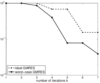
Fig. 2: Ideal and worst-case GMRES can differ from step 3 up to the step $2n-1$.

6 Ideal and worst-case GMRES for complex vectors or polynomials

We now ask whether the values of the max-min approximation (3) and the min-max approximation (4) for a matrix $A\in\mathbb{R}^{n\times n}$ can change if we allow the maximization over complex vectors and/or the minimization over complex polynomials. The answer to this question will show that the two approximation problems indeed are of a different nature.

Let us define

$$\varphi_{k,\mathbb{K},\mathbb{F}}(A)\equiv\min_{p\in\pi_{k,\mathbb{K}}}\max_{{b\in\mathbb{F}^{n}\atop\|b\|=1}}\|p(A)b\|,\qquad\Psi_{k,\mathbb{K},\mathbb{F}}(A)\equiv\max_{{b\in\mathbb{F}^{n}\atop\|b\|=1}}\min_{p\in\pi_{k,\mathbb{K}}}\|p(A)b\|,$$

where $\mathbb{K}$ and $\mathbb{F}$ are either the real or the complex numbers. Hence, the previously used $\varphi_{k}(A)$, $\Psi_{k}(A)$, and $\pi_{k}$ are now denoted by $\varphi_{k,\mathbb{R},\mathbb{R}}(A)$ and $\Psi_{k,\mathbb{R},\mathbb{R}}(A)$, and $\pi_{k,\mathbb{R}}$, respectively. We first analyze the case of $\varphi_{k,\mathbb{K},\mathbb{F}}(A)$.

Theorem 14.

For a nonsingular matrix $A\in\mathbb{R}^{n\times n}$ and $1\leq k\leq d(A)-1$,

$$\varphi_{k,\mathbb{R},\mathbb{R}}(A)=\varphi_{k,\mathbb{C},\mathbb{R}}(A)=\varphi_{k,\mathbb{R},\mathbb{C}}(A)=\varphi_{k,\mathbb{C},\mathbb{C}}(A).$$

Proof.

Since

$$\max_{{b\in\mathbb{R}^{n}\atop\|b\|=1}}\|Bv\|=\|B\|=\max_{{b\in\mathbb{C}^{n}\atop\|b\|=1}}\|Bv\|$$

holds for any real matrix $B\in\mathbb{R}^{n\times n}$, we have $\varphi_{k,\mathbb{R},\mathbb{R}}(A)=\varphi_{k,\mathbb{R},\mathbb{C}}(A).$

Next, from $\mathbb{R}\subset\mathbb{C}$ we get immediately $\varphi_{k,\mathbb{C},\mathbb{R}}(A)\leq\varphi_{k,\mathbb{R},\mathbb{R}}(A).$ On the other hand, writing $p\in\pi_{k,\mathbb{C}}$ in the form $p=p_{r}+\mathbf{i}\>p_{i}$, where $p_{r}\in\pi_{k,\mathbb{R}}$ and $p_{i}$ is a real polynomial of degree at most $k$ such that $p_{i}(0)=0$, we get

$$\varphi_{k,\mathbb{C},\mathbb{R}}^{2}(A)=\min_{p\in\pi_{k,\mathbb{C}}}\max_{{b\in\mathbb{R}^{n}\atop\|b\|=1}}\|p(A)b\|^{2} = \min_{p\in\pi_{k,\mathbb{C}}}\max_{{b\in\mathbb{R}^{n}\atop\|b\|=1}}\,\left(\|p_{r}(A)b\|^{2}+\|p_{i}(A)b\|^{2}\right)$$

$$\geq \min_{p_{r}\in\pi_{k,\mathbb{R}}}\max_{{b\in\mathbb{R}^{n}\atop\|b\|=1}}\|p_{r}(A)b\|^{2}=\varphi_{k,\mathbb{R},\mathbb{R}}^{2}(A),$$

so that $\varphi_{k,\mathbb{C},\mathbb{R}}(A)=\varphi_{k,\mathbb{R},\mathbb{R}}(A).$ Finally, from [5, Theorem 3.1] we obtain $\varphi_{k,\mathbb{R},\mathbb{R}}(A)=\varphi_{k,\mathbb{C},\mathbb{C}}(A).$ ∎

Since the value of $\varphi_{k,\mathbb{K},\mathbb{F}}(A)$ does not change when choosing for $\mathbb{K}$ and $\mathbb{F}$ real or complex numbers, we will again use the simple notation $\varphi_{k}(A)$ in the following text. The situation for the quantities corresponding to the worst-case GMRES approximation is more complicated. Our proof of this fact uses the following lemma.

Lemma 15.

If $A=A(\omega,\varepsilon)$ is the Toh matrix defined in $(\ref{eq:Toh})$ and

$$B\equiv\left[\begin{array}[]{cc}A&0\\ 0&A\end{array}\right],$$ (23)

then $\Psi_{3,\mathbb{R},\mathbb{R}}(B)=\varphi_{3}(A)$.

Proof.

Using the structure of $B$ it is easy to see that $\Psi_{k,\mathbb{R},\mathbb{R}}(B)\leq\varphi_{k}(A)$ for any $k$. To prove the equality, it suffices to find a real unit norm vector $w$ with

$$\min_{p\in\pi_{3,\mathbb{R}}}\|p(B)w\|=\varphi_{3}(A)=\min_{p\in\pi_{3,\mathbb{R}}}\|p(A)\|.$$ (24)

The solution $p_{*}$ of the ideal GMRES problem on the right hand side of (24) is given by (21). Toh showed in [13, p. 32] that $p_{*}(A)$ has a twofold maximal singular value $\sigma$, and that the corresponding right and left singular vectors are given (up to a normalization) by

$$[v_{1},v_{2}]=\left[\begin{array}[]{rr}0&c\\ c&0\\ 0&-2\\ -2&0\end{array}\right],\qquad[u_{1},u_{2}]=\left[\begin{array}[]{rr}0&2\\ 2&0\\ 0&-c\\ -c&0\end{array}\right],$$

i.e., $\sigma u_{1}=p_{*}(A)v_{1}$ and $\sigma u_{2}=p_{*}(A)v_{2},$ where $\sigma=\|p_{*}(A)\|$.

Let us define

$$w\equiv\left[\begin{array}[]{c}v_{1}\\ v_{2}\end{array}\right]/\left\|\left[\begin{array}[]{c}v_{1}\\ v_{2}\end{array}\right]\right\|,\qquad q(z)\equiv p_{*}(z).$$

Using

$$q(B)\left[\begin{array}[]{c}v_{1}\\ v_{2}\end{array}\right]=\sigma\left[\begin{array}[]{c}u_{1}\\ u_{2}\end{array}\right]\quad\mbox{and}\quad\left\|\left[\begin{array}[]{c}v_{1}\\ v_{2}\end{array}\right]\right\|=\left\|\left[\begin{array}[]{c}u_{1}\\ u_{2}\end{array}\right]\right\|,$$

we see that $\left\|q(B)w\right\|=\sigma.$ To prove (24) it is sufficient to show that $q$ is the third GMRES polynomial for $B$ and $w$, i.e., that $q$ satisfies $q(B)w\perp B^{j}w$ for $j=1,2,3$, or, equivalently,

$$\left[\begin{array}[]{c}u_{1}\\ u_{2}\end{array}\right]^{T}\left[\begin{array}[]{cc}A^{j}&0\\ 0&A^{j}\end{array}\right]\left[\begin{array}[]{c}v_{1}\\ v_{2}\end{array}\right]=u_{1}^{T}A^{j}v_{1}+u_{2}^{T}A^{j}v_{2}=0,\quad j=1,2,3.$$

Using linear algebra calculations we get $u_{1}^{T}Av_{1}=-4c=-u_{2}^{T}Av_{2}$, and

$$0=u_{1}^{T}A^{2}v_{1}=u_{2}^{T}A^{2}v_{2}=u_{1}^{T}A^{3}v_{1}=u_{2}^{T}A^{3}v_{2}.$$

Therefore, we have found a unit norm initial vector $w$ and the corresponding third GMRES polynomial $q$ such that $\|q(B)w\|=\varphi_{3}(A).$  ∎

We next analyze the quantities $\Psi_{k,\mathbb{K},\mathbb{F}}(A)$.

Theorem 16.

For a nonsingular matrix $A\in\mathbb{R}^{n\times n}$ and $1\leq k\leq d(A)-1$,

$$\Psi_{k,\mathbb{R},\mathbb{R}}(A)=\Psi_{k,\mathbb{C},\mathbb{R}}(A)\leq\Psi_{k,\mathbb{C},\mathbb{C}}(A)\leq\Psi_{k,\mathbb{R},\mathbb{C}}(A)\,,$$

where both inequalities can be strict.

Proof.

For a real initial vector $b$, the corresponding GMRES polynomial is uniquely determined and real. This implies $\Psi_{k,\mathbb{C},\mathbb{R}}(A)=\Psi_{k,\mathbb{R},\mathbb{R}}(A).$ Next, from [5, Theorem 3.1] it follows that $\Psi_{k,\mathbb{R},\mathbb{R}}(A)\leq\Psi_{k,\mathbb{C},\mathbb{C}}(A).$ Finally, using $\mathbb{R}\subset\mathbb{C}$ we get $\Psi_{k,\mathbb{C},\mathbb{C}}(A)\leq\Psi_{k,\mathbb{R},\mathbb{C}}(A).$

It remains to show that the inequalities can be strict. For the first inequality, as shown in [16, Section 4], there exist real matrices $A$ and certain complex (unit norm) initial vectors $b$ for which $\min_{p\in\pi_{k,\mathbb{C}}}\,\|p(A)b\|=1$ for $k=1,\dots,n-1$ (complete stagnation), while such complete stagnation does not occur for any real (unit norm) initial vector. Therefore, there are matrices for which $\Psi_{k,\mathbb{C},\mathbb{R}}(A)<\Psi_{k,\mathbb{C},\mathbb{C}}(A)$.

To show that the second inequality can be strict, we note that for any $A\in\mathbb{R}^{n\times n}$, the corresponding matrix $B\in\mathbb{R}^{2n\times 2n}$ of the form (23), and $1\leq k\leq d(A)-1$,

$$\Psi^{2}_{k,\mathbb{R},\mathbb{C}}(A) = \max_{{b\in\mathbb{C}^{n}\atop\|b\|=1}}\min_{p\in\pi_{k,\mathbb{R}}}\|p(A)b\|^{2}=\max_{{u,v\in\mathbb{R}^{n}\atop\|u\|^{2}+\|v\|^{2}=1}}\min_{p\in\pi_{k,\mathbb{R}}}\|p(A)(u+\,\mathbf{i}\,v)\|^{2}$$ (25)

$$= \max_{{u,v\in\mathbb{R}^{n}\atop\|u\|^{2}+\|v\|^{2}=1}}\min_{p\in\pi_{k,\mathbb{R}}}\,(\|p(A)u\|^{2}+\|p(A)v\|^{2})$$

$$= \max_{{v\in\mathbb{R}^{2n}\atop\|v\|=1}}\min_{p\in\pi_{k,\mathbb{R}}}\|p(B)v\|^{2}\;=\;\Psi^{2}_{k,\mathbb{R},\mathbb{R}}(B).$$

Now let $A$ be the Toh matrix $(\ref{eq:Toh})$ and $k=3$. Toh showed in [13, Theorem 2.2] that for any unit norm $b\in\mathbb{C}^{4}$ and the corresponding third GMRES polynomial $p_{b}\in\pi_{3,\mathbb{C}}$,

$$\|p_{b}(A)b\|<\varphi_{3}(A).$$

Hence $\Psi_{3,\mathbb{C},\mathbb{C}}(A)<\varphi_{3}(A)$. Lemma 15 and equation (25) imply $\varphi_{3}(A)=\Psi_{3,\mathbb{R},\mathbb{C}}(A)$, which completes the proof of the strict inequality.   ∎

Our proof concerning the strictness of the first inequality in the previous theorem relied on a numerical example given in [16, Section 4]. We will now give an alternative construction based on the non-uniqueness of the worst-case GMRES polynomial, which will lead to an example with

$$\Psi_{k,\mathbb{R},\mathbb{R}}(A)<\Psi_{k,\mathbb{R},\mathbb{C}}(A).$$

Suppose that $A$ is a real matrix for which in a certain step $k$ two different worst-case polynomials $p_{b}\in\pi_{k,\mathbb{R}}$ and $p_{c}\in\pi_{k,\mathbb{R}}$ with corresponding real unit norm initial vectors $b$ and $c$ exist, so that

$$\Psi_{k,\mathbb{R},\mathbb{R}}(A)\,=\,\|p_{b}(A)b\|\,=\,\|p_{c}(A)c\|.$$

Note that since $p_{b}$ and $p_{c}$ are the uniquely determined GMRES polynomials that solve the problem (1) for the corresponding real initial vectors, it holds that

$$\|p_{b}(A)b\|<\|p(A)b\|,\qquad\|p_{c}(A)c\|<\|p(A)c\|$$ (26)

for any polynomial $p\in\pi_{k,\mathbb{C}}\setminus\{p_{b},p_{c}\}$.

Writing any complex vector $w\in\mathbb{C}^{n}$ in the form $w=(\cos\theta)\,u\,+\,\mathbf{i}\,(\sin\theta)\,v$, with $u,v\in\mathbb{R}^{n}$, $\|u\|=\|v\|=1,$ we get

$$\Psi^{2}_{k,\mathbb{R},\mathbb{C}}(A) = \max_{w\in\mathbb{C}^{n}\atop\|w\|=1}\min_{p\in\pi_{k,\mathbb{R}}}\,\|p(A)b\|^{2}$$

$$= \max_{\theta\in\mathbb{R},u,v\in\mathbb{R}^{n}\atop\|u\|=\|v\|=1}\min_{p\in\pi_{k,\mathbb{R}}}\,\left(\cos^{2}\theta\,\|p(A)u\|^{2}+\sin^{2}\theta\,\|p(A)v\|^{2}\right)$$

$$\geq \max_{\theta\in\mathbb{R}}\min_{p\in\pi_{k,\mathbb{R}}}\,\left(\cos^{2}\theta\|p(A)b\|^{2}+\sin^{2}\theta\|p(A)c\|^{2}\right)$$

$$> (\cos^{2}\theta)\,\Psi^{2}_{k,\mathbb{R},\mathbb{R}}(A)\,+\,(\sin^{2}\theta)\,\Psi^{2}_{k,\mathbb{R},\mathbb{R}}(A)=\Psi^{2}_{k,\mathbb{R},\mathbb{R}}(A),$$

where the strict inequality follows from (26) and from the fact that $\|p(A)b\|^{2}$ and $\|p(A)c\|^{2}$ do not attain their minima for the same polynomial.

To demonstrate the strict inequality $\Psi_{k,\mathbb{R},\mathbb{R}}(A)<\Psi_{k,\mathbb{R},\mathbb{C}}(A)$ numerically we use the Toh matrix $(\ref{eq:Toh})$ with $\varepsilon=0.1$ and $\omega=1$, and $k=3$. Let $b$ and $c$ be the corresponding two different worst-case initial vectors introduced in Section 4. We vary $\theta$ from $0$ to $\pi$ and compute the quantities

$$\min_{p\in\pi_{3,\mathbb{R}}}\,\left(\cos^{2}\theta\,\|p(A)b\|^{2}+\sin^{2}\theta\,\|p(A)c\|^{2}\right)=\min_{p\in\pi_{3,\mathbb{R}}}\,\|p(B)g_{\theta}\|^{2},$$ (27)

where

$$B=\left[\begin{array}[]{cc}A&0\\ 0&A\end{array}\right]\quad\mbox{and}\quad g_{\theta}=\left[\begin{array}[]{c}(\cos\theta)b\\ (\sin\theta)c\end{array}\right].$$

In Fig. 3 we can see clearly, that for $\theta\notin\{0,\,\pi/2\,,\pi\}$ the value of (27) is strictly larger than $\Psi_{3}(A)=0.4579$.

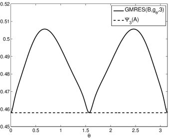
Fig. 3: The GMRES residual norm for a varying complex right hand side.

7 Concluding remarks

We have studied the worst-case GMRES approximation problem, which for each (nonsingular) matrix $A$ and iteration step $k\leq d(A)$ represents the best possible attainable upper bound on the actual GMRES residual norm for a linear algebraic system with $A$ at step $k$. We have derived several theoretical properties of the worst-case GMRES problem, and we have studied its relation to the ideal GMRES approximation problem.

In this paper we did not consider quantitative estimation of the worst-case GMRES value $\Psi_{k}(A)$, and we did not study how this value depends on properties of $A$. This is an important problem of great practical interest, which is largely open. For more details and a survey of the current state-of-the-art we refer to [8, Section 5.7].

References

[1]V. Faber, W. Joubert, E. Knill, and T. Manteuffel, Minimal residual
method stronger than polynomial preconditioning, SIAM J. Matrix Anal. Appl.,
17 (1996), pp. 707–729.
[2]A. Greenbaum, Iterative Methods for Solving Linear Systems,
vol. 17 of Frontiers in Applied Mathematics, SIAM, Philadelphia, PA, 1997.
[3]A. Greenbaum and L. Gurvits, Max-min properties of matrix factor
norms, SIAM J. Sci. Comput., 15 (1994), pp. 348–358.
[4]Anne Greenbaum and Lloyd N. Trefethen, GMRES/CR and
Arnoldi/Lanczos as matrix approximation problems, SIAM J. Sci. Comput.,
15 (1994), pp. 359–368.
[5]Wayne Joubert, On the convergence behavior of the restarted GMRES
algorithm for solving nonsymmetric linear systems, Numer. Linear Algebra
Appl., 1 (1994), pp. 427–447.
[6], A robust
GMRES-based adaptive polynomial preconditioning algorithm for nonsymmetric
linear systems, SIAM J. Sci. Comput., 15 (1994), pp. 427–439.
[7]Peter D. Lax, Linear Algebra and its Applications, Pure and
Applied Mathematics (Hoboken), Wiley-Interscience [John Wiley & Sons],
Hoboken, NJ, second ed., 2007.
[8]J. Liesen and Z. Strakoš, Krylov Subspace Methods.
Principles and Analysis, Oxford University Press, Oxford, 2013.
[9]Jörg Liesen and Petr Tichý, On best approximations of
polynomials in matrices in the matrix 2-norm, SIAM J. Matrix Anal. Appl., 31
(2009), pp. 853–863.
[10]Yousef Saad, Iterative Methods for Sparse Linear Systems,
SIAM, Philadelphia, PA, second ed., 2003.
[11]Yousef Saad and Martin H. Schultz, GMRES: a generalized minimal
residual algorithm for solving nonsymmetric linear systems, SIAM J. Sci.
Statist. Comput., 7 (1986), pp. 856–869.
[12]Petr Tichý, Jörg Liesen, and Vance Faber, On worst-case
GMRES, ideal GMRES, and the polynomial numerical, hull of a Jordan
block, Electron. Trans. Numer. Anal., 26 (2007), pp. 453–473.
[13]Kim-Chuan Toh, GMRES vs. ideal GMRES, SIAM J. Matrix Anal.
Appl., 18 (1997), pp. 30–36.
[14]Kim-Chuan Toh and Lloyd N. Trefethen, The Chebyshev polynomials of
a matrix, SIAM J. Matrix Anal. Appl., 20 (1998), pp. 400–419.
[15]Ilya Zavorin, Spectral factorization of the Krylov matrix and
convergence of GMRES, Tech. Report CS-TR-4309, Computer Science
Department, University of Maryland, 2001.
[16]Ilya Zavorin, Dianne P. O’Leary, and Howard Elman, Complete
stagnation of GMRES, Linear Algebra Appl., 367 (2003), pp. 165–183.