Stochastic coupling in two modes systems: the weak-strong coupling transition

Abstract

We investigate the weak-strong coupling transition of two linearly coupled systems under the influence of a phase fluctuating coupling. In the weak coupling regime the exponential decay of quantum properties is well known. A different scenario occurs in the strong coupling regime, the inhibition of the dynamics which tends to “freeze” as the ration between coupling strength and average phase fluctuation time increase. Exciton-polariton oscillations and the self-trapping phenomenon in Bose-Einstein Condensate qualitatively illustrate the weak and strong regimes respectively.

1 Introduction

Decoherence effects are now believed to be the essential ingredient which destroys most of the counterintuitive aspects of quantum mechanics. Such effects are at the same time an academic tool to the understanding of the classical limit of quantum mechanics as well as an important ingredient in the area of quantum computation. The dynamics of quantum open systems has been therefore extensively studied [1]. Of particular importance in this context is the Born-Markov approximation which leads to master equations of various kinds [2], whose validity is limited by the weak coupling approximation. The strong coupling regime however has been less explored.

It is the purpose of the present contribution to shed some light onto the weak-strong coupling transition in the context of two linearly interacting systems under the influence of a phase fluctuating coupling. The model in spite of its schematic character has been shown in several instances and different areas to reflect and adequately describe experimental results. Examples are the description of exciton-polariton damped oscillations [3, 4]; predictions for the behavior of oscillations of two coupled modes in the context of microwave cavities [5, 6]; the self-trapping phenomenon in the tunneling process of a Bose-Einstein condensate (BEC) [7, 8, 9, 10, 11, 12, 13, 14].

We will show that in the weak coupling regime the usual master equation results are recovered and the usual phenomenological damping constant is derived as a function of the model parameters. The strong coupling limit however leads to a completely different scenario, the “freezing” of the dynamics. We will illustrate these effects in the context of exciton-polariton oscillations and the self-trapping of a BEC in a devised laser potential.

2 The Model

In this section we give a detailed derivation of the stochastic time evolution of the following system

$$H=\hbar\omega_{a}a^{{\dagger}}a+\hbar\omega_{b}b^{{\dagger}}b+\hbar\big{[}g(t)a^{{\dagger}}b+g^{*}(t)b^{{\dagger}}a\big{]},$$ (1)

where $a^{{\dagger}}(a)$ and $b^{{\dagger}}(b)$ are creation (annihilation) operators. $\omega_{a}$ and $\omega_{b}$ are the frequencies of the a-mode and b-mode respectively. Since that the operators $a$ and $b$ were considered as bosons they will obey the commutation relation for bosons $[a,a^{{\dagger}}]=1$ and $[b,b^{{\dagger}}]=1$. In the third term, $g(t)$ stands for the interaction strength between the modes and here is assumed to be time dependent in the sence that $|g(t)|$ is constant but its phase is a stochastic variable. The Hamiltonian (1) can be written in matrix form

$$H = \hbar\left(\begin{array}[]{cc}a^{{\dagger}}&b^{{\dagger}}\end{array}\right)\left(\begin{array}[]{cc}\omega_{a}&g(t)\\ g^{*}(t)&\omega_{b}\\ \end{array}\right)\left(\begin{array}[]{cc}a\\ b\end{array}\right).$$ (7)

The time evolution operator for the system is given by

$$U(t) = e^{-iH_{int}t/\hbar}$$ (10)

$$= \left(\begin{array}[]{cc}\cos\big{(}|g|t\big{)}&\frac{g(t)}{|g|}\sin\big{(}|g|t\big{)}\\ -\frac{g^{*}(t)}{|g|}\sin\big{(}|g|t\big{)}&\cos\big{(}|g|t\big{)}\\ \end{array}\right),$$

where $H_{int}$ is the interaction part of the Hamiltonian $H$.

We will specify the noise by defining a stochastic process for $\phi(t)$. In our model we assume that

$$g(t)=g_{0}\exp\big{[}i\phi(t)\big{]},$$ (11)

where $g_{0}$ is the non-stochastic amplitude while the phase $\phi(t)$ is treated as a stochastic variable. Here, we will consider random phase telegraph noise where $\phi(t)$ itself fluctuates in the manner of jumps. In particular, the phase fluctuations were describe by a Wierner-Levy (phase diffusion) process and the amplitude fluctuations by a colored gaussian noise. An alternative model which represents noise by means of discrete jump processes was first introduced into quantum optics by Burshtein and Oseledchik [15]. A simple example of such a jump process is the two-state random telegraph. These models are very convenient and elegant to study the noise of the electromagnetic atom-field interaction in a non-perturbative manner. The random telegraph models, whether associated with phase, frequency or amplitude fluctuations lead to an equation for average responses in exact algebraic form. The model of random telegraph (jump-type) noise is physically very sound to describe the noise arising from electromagnetic field fluctuation or from collisions of various kinds or from other external sources. Indeed, that model including the effects of stochastic phase and/or in amplitude has been explicitly solved for the case of the James-Cumming model (JCM) by A. Joshi [16]. The fluctuations are modeled by the random telegraph process and an equation for the density operator averaged over the fluctuations is obtained. The solution of these equations was used to study the decoherence effects in the dynamics of the system. A. Joshi’s work was treated in a pedagogical form by E. A. Ospina [17]. We assume further that the change in $\phi(t)$ occurs instantaneously jump wise and the jumps are separated by mean time intervals of the order $\tau_{0}$ in which $\phi(t)=$ constant, as shown in Fig. (1).

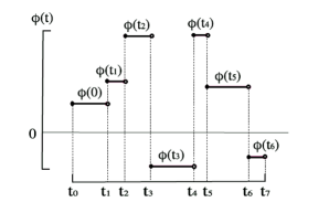
Figure 1: Schematic representation of the phase distribution of coupling between the modes.

There are two stochastic variables: the time interval $\tau$ between one and the next jump and the value of the phase constant $\phi$ in each of these intervals. The variable $\tau=t_{i}-t_{i-1}$ follow the probability distribution

$$dQ(\tau)=\frac{1}{\tau_{0}}e^{-\tau/\tau_{0}}d\tau.$$ (12)

with $t_{0}=0$. The above distribution specifies the probability of duration of each such jump interval and has intervals mean duration $\tau_{0}$. We consider only the case in which the phases $\phi(t)$ are uncorrelated. The probability distribution to phase is given by

$$dq(\phi)=\frac{d\phi}{2\pi},$$ (13)

with mean value $\langle\phi\rangle=\pi$. So, at any instant, the probability of finding a given $\phi$ remains the same and equation to $dQ(t)$, and there is no limitation on the form of this distribution. In other words, $\phi(t)$ is undergoing random continuous change of Markov type.

The dynamics of the system is given by the unitary transformation $U(\phi,t,t^{{}^{\prime}})$ such that

$$\rho(t;\phi)=U(\phi,t,t^{{}^{\prime}})\rho(t^{{}^{\prime}})U^{-1}(\phi,t,t^{{}^{\prime}}).$$ (14)

At the end of each (ith) interval we find the density matrix $\rho(t)$ which is the initial condition for the next matrix, so, if in the interval $(0,t)$ there are $k$ jumps in $\phi$, then

$$\rho(t;t_{1},\cdots, t_{k} ,\phi_{0},\cdots,\phi_{k})=U(\phi_{k};t,t_{k})U(\phi_{k-1};t_{k},t_{k-1})\cdots$$ (15)

$$\times U(\phi_{1};t_{2},t_{1})U(\phi_{0};t_{1},0)\rho(0)U^{-1}(\phi_{0};t_{1},0)U^{-1}(\phi_{1};t_{2},t_{1})\cdots$$

$$\times U^{-1}(\phi_{k-1};t_{k},t_{k-1})U^{-1}(\phi_{k};t,t_{k}).$$

The above expression is of multiplicative nature and hence it is quite easy to average over. The probability (in the interval $(0,t)$) that $k$ changes of $\phi$ have actually occurred at successive instants $t_{1},t_{2},\cdots,t_{k}$ and that a certain sequence of $\phi_{1},\phi_{2},\cdots,\phi_{k}$ (where $\phi_{i}=\phi(t_{i})$) was realized between them is obviously equal to

$$dP(t_{1},t_{2},\cdots,t_{k};\phi_{1},\phi_{2},\cdots,\phi_{k},t)=\frac{1}{\tau^{k}_{0}}e^{-t/\tau_{0}}\Big{(}\prod_{i=1}^{k}dt_{i}\Big{)}\Big{(}\prod_{i=1}^{k}dq(\phi_{i})\Big{)}.$$ (16)

The average density operator can thus be written as

$$\bar{\rho}(t)=\sum_{k=0}^{\infty}\int\int dP(t_{1},t_{2},\cdots,t_{k};\phi_{1},\phi_{2},\cdots,\phi_{k},t)\rho(t;t_{1},\cdots, t_{k} ,\phi_{0},\cdots,\phi_{k}).$$

Rewrite (LABEL:eqrho_comp) with use of (16) we get

$$\bar{\rho}(t)e^{t/\tau_{0}} = \sum_{k=0}^{\infty}\frac{1}{\tau^{k}_{0}}\int_{0}^{t}dt_{k}\int_{0}^{t_{k}}dt_{k-1}\cdots\int_{0}^{t_{2}}dt_{1}\int dq(\phi_{k})\int dq(\phi_{k-1})\cdots$$ (18)

$$\times \int dq(\phi_{0})\rho(t;t_{1},\cdots,t_{k},\phi_{0},\cdots,\phi_{k}).$$

Note that the term with $k=0$ (when $\phi$ does not change at all in the interval $(0,t)$) will not contain integrals with respect to time and thus is given by

$$\int dq(\phi_{0})\rho(t,\phi_{0}).$$ (19)

Now using the recurrence relation (14), we can multiply both sides of equation (18) from the left (right) by $U^{-1}(\phi;\tau,t)$ ($U(\phi;\tau,t)$) respectively and also by $dq(\phi)dt/\tau_{0}$, then integrate with respect to time from $0$ to $\tau$ and eliminate the entire series using equation (18). After some simplifications it is easy to show that

$$\bar{\rho}(\tau)e^{\tau/\tau_{0}} = \int dq(\phi_{0})U(\phi_{0};\tau,0)\rho(0)U^{-1}(\phi_{0};\tau,0)$$ (20)

$$+ \frac{1}{\tau_{0}}\int_{0}^{\tau}dte^{t/\tau_{0}}\int dq(\phi)U(\phi;\tau,t)\bar{\rho}(t)U^{-1}(\phi;\tau,t).$$

Now we will rewrite the equation (20) above in term of matrix elements of operators $\bar{\rho}(\tau)$ and $U(\phi;\tau,t)$

$$\bar{\rho}(\tau)_{im}e^{\tau/\tau_{0}} = \int dq(\phi_{0})\sum_{k,l}U(\phi_{0};\tau,0)_{ik}\rho(0)_{kl}U^{-1}(\phi_{0};\tau,0)_{lm}$$ (21)

$$+ \frac{1}{\tau_{0}}\int_{0}^{\tau}dte^{t/\tau_{0}}\int dq(\phi)\sum_{k,l}U(\phi;\tau,t)_{ik}\bar{\rho}(t)_{kl}U^{-1}(\phi;\tau,t)_{lm}.$$

Define the conjunct of matrix $\{\mathbb{G}^{im}(\tau,t)\}$ with elements give by

$$G^{im}(\tau,t)_{lk} = \int dq(\phi)U_{ik}(\phi;\tau,t)U_{lm}^{-1}(\phi;\tau,t),$$ (22)

so

$$\bar{\rho}(\tau)_{im}e^{\tau/\tau_{0}} = \sum_{l}\Big{[}\sum_{k}G^{im}(\tau,0)_{lk}\rho(0)_{kl}\Big{]}$$ (23)

$$+ \frac{1}{\tau_{0}}\int_{0}^{\tau}dte^{t/\tau_{0}}\sum_{l}\Big{[}\sum_{k}G^{im}(\tau,t)_{lk}\bar{\rho}(t)_{kl}\Big{]}$$

$$= \sum_{l}[\mathbb{G}^{im}(\tau,0)\rho(0)]_{ll}$$

$$+ \frac{1}{\tau_{0}}\int_{0}^{\tau}dte^{t/\tau_{0}}\sum_{l}[\mathbb{G}^{im}(\tau,t)\bar{\rho}(t)]_{ll}.$$

Using the trace definition $TrA=\sum_{l}a_{ll}$ we get

$$\bar{\rho}(\tau)_{im} = e^{-\tau/\tau_{0}}Tr\big{[}\mathbb{G}^{im}(\tau,0)\rho(0)\big{]}$$ (24)

$$+ \frac{1}{\tau_{0}}\int_{0}^{\tau}dte^{-(\tau-t)/\tau_{0}}Tr\big{[}\mathbb{G}^{im}(\tau,t)\bar{\rho}(t)\Big{]}.$$

This is the statistical average over the random variable $\phi(t)$. In order to determine the dynamical evolution of the system one has to determine $\mathbb{G}$. The problem is now simplified because we have to deal with interval in which $\phi$ (or alternatively $g$) is constant and the change in $\rho$ is perfectly regular. Thus, knowing $\mathbb{G}$, we can find the average variation of the system during the relaxation process [15]. To determine $\mathbb{G}$ we will use the time evolution operator $U(t)$ given by (10) with $g(t)$ defined in (11)

$$U(t) = \left(\begin{array}[]{cc}\cos\big{(}|g|t\big{)}&e^{i\phi}\sin\big{(}|g|t\big{)}\\ -e^{-i\phi}\sin\big{(}|g|t\big{)}&\cos\big{(}|g|t\big{)}\\ \end{array}\right).$$ (27)

The elements to be averaged in the calculations of $\mathbb{G}$ are those containing the factors $e^{\pm i\phi}$. Since the phases are equally probable most of the terms vanish after averaging. The remaining (relevant for our purposes) non-vanishing elements of $\mathbb{G}$ are

$$G_{11}^{11} = G_{22}^{22}=\cos^{2}\big{[}(g_{0}(\tau-t)\big{]}$$

$$G_{22}^{11} = G_{11}^{22}=\sin^{2}\big{[}(g_{0}(\tau-t)\big{]}$$ (28)

$$G_{21}^{12} = G_{12}^{21}=\cos^{2}\big{[}(g_{0}(\tau-t)\big{]}.$$

We have thus

$$G^{11}(\tau,t) = \left(\begin{array}[]{cc}\cos^{2}\big{[}(g_{0}(\tau-t)\big{]}&0\\ 0&\sin^{2}\big{[}(g_{0}(\tau-t)\big{]}\\ \end{array}\right)$$ (31)

$$G^{12}(\tau,t) = \left(\begin{array}[]{cc}0&0\\ \cos^{2}\big{[}(g_{0}(\tau-t)\big{]}&0\\ \end{array}\right)=\big{[}G^{21}(\tau,t)\big{]}^{T}$$ (34)

$$G^{22}(\tau,t) = \left(\begin{array}[]{cc}\sin^{2}\big{[}(g_{0}(\tau-t)\big{]}&0\\ 0&\cos^{2}\big{[}(g_{0}(\tau-t)\big{]}\\ \end{array}\right),$$ (37)

and using equations (24) and (34) we obtain

$$\bar{\rho}(\tau)_{11}e^{\tau/\tau_{0}} = \rho(0)_{11}+\big{[}\rho(0)_{22}-\rho(0)_{11}\big{]}\sin^{2}\big{(}g_{0}\tau\big{)}$$

$$+ \frac{1}{\tau_{0}}\int_{0}^{\tau}dte^{t/\tau_{0}}\big{\{}\bar{\rho}(t)_{11}+\big{[}\bar{\rho}(t)_{22}-\bar{\rho}(t)_{11}\big{]}\sin^{2}\big{[}g_{0}(\tau-t)\big{]}\big{\}},$$

$$\bar{\rho}(\tau)_{22}e^{\tau/\tau_{0}} = \rho(0)_{22}+\big{[}\rho(0)_{11}-\rho(0)_{22}\big{]}\sin^{2}\big{(}g_{0}\tau\big{)}$$

$$+ \frac{1}{\tau_{0}}\int_{0}^{\tau}dte^{t/\tau_{0}}\big{\{}\bar{\rho}(t)_{22}+\big{[}\bar{\rho}(t)_{11}-\bar{\rho}(t)_{22}\big{]}\sin^{2}\big{[}g_{0}(\tau-t)\big{]}\big{\}}.$$

3 Dynamics of the average number of a mode

The average bosons number is given by

$$n_{a}(t)=Tr\Big{[}\rho(t)a^{{\dagger}}a\Big{]}$$ (39)

and can be evaluated using equations (2):

$$\langle\overline{n_{a}(\tau)}\rangle e^{\tau/\tau_{0}} = \langle n_{a}(0)\rangle\Big{[}1-2\sin^{2}\big{(}g_{0}\tau\big{)}\Big{]}+\langle N\rangle\sin^{2}\big{(}g_{0}\tau\big{)}$$

$$+ \frac{1}{\tau_{0}}\int_{0}^{\tau}e^{t/\tau_{0}}\langle\overline{n_{a}(t)}\rangle\Big{\{}1-2\sin^{2}\big{[}g_{0}(\tau-t)\big{]}\Big{\}}dt$$

$$+ \frac{\langle N\rangle}{\tau_{0}}\int_{0}^{\tau}e^{t/\tau_{0}}\sin^{2}\big{[}g_{0}(\tau-t)\big{]}dt,$$

where $\langle N\rangle=\langle n_{a}(0)\rangle+\langle n_{b}(0)\rangle$ is the initial excitation number with $\langle n_{a}(0)\rangle$ and $\langle n_{b}(0)\rangle$ being the average excitations in each mode. This equation describes the relaxation of the intensity of the mode $a$ and can be solved using the Laplace transform. To solve (3) we will define

$$f(t) = \langle\overline{n_{a}(t)}\rangle e^{t/\tau_{0}},$$

$$g(t) = 1-2\sin^{2}\big{(}g_{0}t\big{)}=\cos\big{(}2g_{0}t\big{)},$$

$$h(t) = e^{t/\tau_{0}},$$

$$j(t) = \sin^{2}\big{(}g_{0}t\big{)}.$$

inserting the functions defined above into (3) we obtain

$$f(\tau) = \langle n_{a}(0)\rangle g(\tau)+\frac{1}{\tau_{0}}\int_{0}^{\tau}f(t)g(\tau-t)dt$$ (41)

$$+ \langle N\rangle j(\tau)+\frac{\langle N\rangle}{\tau_{0}}\int_{0}^{\tau}h(t)j(\tau-t)dt.$$

Now applying the Laplace transform on both sides of (41) we obtain

$$\hat{f}(s) = \langle n_{a}(0)\rangle\hat{g}(s)+\frac{1}{\tau_{0}}\hat{f}(s)\hat{g}(s)$$

$$+ \langle N\rangle\hat{j}(s)+\frac{\langle N\rangle}{\tau_{0}}\hat{h}(s)\hat{j}(s)$$

$$= \frac{\langle n_{a}(0)\rangle\hat{g}(s)+\langle N\rangle\hat{j}(s)+\frac{\langle N\rangle}{\tau_{0}}\hat{h}(s)\hat{j}(s)}{\Big{[}1-\frac{1}{\tau_{0}}\hat{g}(s)\Big{]}}.$$

Calculating the Laplace transform of the functions $\hat{g}(s)$, $\hat{h}(s)$ and $\hat{j}(s)$ and substituting it into (3) we obtain

$$\hat{f}(s) = \frac{\langle n_{a}(0)\rangle s}{\Big{(}s-\frac{1}{2\tau_{0}}\Big{)}^{2}+\Omega^{2}}+\frac{\langle N\rangle\big{(}2g_{0})^{2}}{2\Big{(}s-\frac{1}{\tau_{0}}\Big{)}}\frac{1}{\Big{[}\Big{(}s-\frac{1}{2\tau_{0}}\Big{)}^{2}+\Omega^{2}\Big{]}},$$ (43)

where we defined $\Omega=\sqrt{(2g_{0})^{2}-\frac{1}{(2\tau_{0})^{2}}}$. The inverse Laplace transform of Eq.(43) yields the following expression the time evolution of the relaxation as

$$\overline{\langle n_{a}(t)\rangle} = \langle n_{a}(0)\rangle e^{-t/2\tau_{0}}\Big{[}\cos\big{(}\Omega t\big{)}+\frac{\sin\big{(}\Omega t\big{)}}{2\tau_{0}\Omega}\Big{]}$$ (44)

$$+ \frac{\langle N\rangle e^{-t/2\tau_{0}}}{2}\Big{\{}\Big{[}e^{t/2\tau_{0}}-\cos\big{(}\Omega t\big{)}\Big{]}-\frac{\sin\big{(}\Omega t\big{)}}{2\tau_{0}\Omega}\Big{\}}.$$

In the limit when the average time $\tau_{0}$ between phase jumps is large as compared with the oscillation period one obtains for $g_{0}\tau_{0}\rightarrow\infty$ a pure oscillatory regime with frequency $2g_{0}$. As the average time between frequency jumps increases one obtains an envelop limiting the oscillation amplitudes and the oscillation frequency is only slightly altered. However in the limit where the average time between jumps decreases as compared with the coupling $g_{0}$ the oscillation ceases at $g_{0}\tau_{0}=0.25$ and an over damped limit sets in. Figures (2) and (3) illustrate the weak coupling regime ($g_{0}\tau_{0}\gg 0.25$) and strong coupling regime ($g_{0}\tau_{0}>0.25$) respectively. Figure (4) illustrates the “freezing” of the dynamics as $g_{0}\tau_{0}$ decreases beyond the limit $g_{0}\tau_{0}=0.25$. The fluctuating interact records information of the system. The information transfer plays the role of unobserved detection process [18]. In our case small values of $g_{0}\tau_{0}$ would imply according to this reasoning that the system is being “measured” with increasing frequency, freezing out as a Zeno like effect.

4 Applications

4.1 The weak coupling regime: Exciton-polariton oscillations

Let us consider the weak coupling regime (WCR), where $g_{0}\tau_{0}>0.25$, and consequently $\Omega$ is a real number. Note that, as $\tau_{0}\rightarrow\infty$, the expression for $\overline{\langle n_{a}(t)\rangle}$ reduces to the usual result without fluctuations. The effects of phase fluctuation in the intensity of the mode $a$ , e.g, for an initial number state $|\varphi(0)\rangle_{b}=|N_{b}\rangle$ and the mode $a$ in vacuum state are given, according to (44), by

$$\overline{\langle n_{a}(t)\rangle} = \frac{N_{b}e^{-t/2\tau_{0}}}{2}\Big{\{}\Big{[}e^{t/2\tau_{0}}-\cos\big{(}\Omega t\big{)}\Big{]}-\frac{\sin\big{(}\Omega t\big{)}}{2\tau_{0}\Omega}\Big{\}}.$$ (45)

The result above shows that the intensity of the mode $a$ contains two parts: (1) Rabi oscillations with frequency $\Omega$; (2) a comparatively slow-varying part $e^{-t/2\tau_{0}}$. To see this more clearly, we plot equation (45) in Figs. (2) and (3) for $N_{b}=2$. It is clear that the damping of Rabi oscillations is more pronounced when the mean time interval $\tau_{0}$ between phase jumps become shorter and shorter until $g_{0}\tau_{0}=0.25$ (see Figures (2) and (3)). In other words the decoherence mechanism is faster for shorter-phase jump intervals.

In this section we compare the results obtained in Ref. [4] which describe the exciton-polariton oscillations in the weak coupling regime with a phenomenological coupling constant. In a real cavity, the modes of exciton and photon are coupled to a continuum of modes which leads to dissipation. The coupling can be scattering of phonons in the case of exciton or cavity damping in the case of photon. In both cases, the result is to dampen the mode of interest. The result obtained in Ref. [4] can be read of Eq.(45) where the damping coefficient corresponds to $\tau_{0}=\gamma^{-1}=(\gamma_{p}+\gamma_{ex})^{-1}$, where $\gamma_{ex}$ and $\gamma_{p}$ are exciton and photon damping from the reservoirs. Using the values of $\gamma$ adopted in Ref. [4] we may estimate the order of magnitude of $\tau_{0}$ as $10^{-10}s$. The model has been shown to reproduce experimental results [19, 20]. In this situation equation (45) can be written as

$$\overline{\langle n_{a}(t)\rangle} = \frac{N_{b}}{2}\Big{[}1-e^{-\gamma t/2}\cos\big{(}2g_{0}t\big{)}\Big{]}.$$ (46)

The results obtained here describe the decoherence process in the system. However, the fluctuations introduce a finite width in the transmission spectrum even in a lossless cavity. On the other hand, in recent work, S. Schneider et al., [21] also included fluctuation in intensity and phase in the exciting laser pulse to explain effects of decoherence for single trapped ion. In Schneider’s model the intensity and phase fluctuations define a stochastic Schrödinger equation in the Ito formalism [22], or more appropriately a stochastic Liouville-von Neumann equation. The results are in good qualitative agreement with recent ion experiments [23].

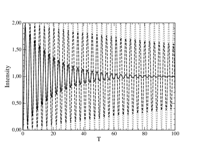
Figure 2: Light intensity as a function of dimensionless time $T=g_{0}t$ for the case that the excitons are initially in a number state $N=2$ for $g_{0}\tau_{0}\rightarrow\infty$ (dotted line), $g_{0}\tau_{0}=100$ (dashed line) and $g_{0}\tau_{0}=10$ (solid line). The intensity is in arbitrary units.

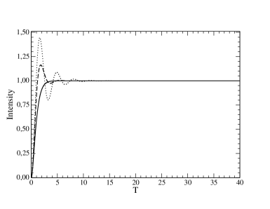
Figure 3: Light intensity as a function of dimensionless time $T=g_{0}t$ for the case that the excitons are initially in a number state $N_{b}=2$ for $g_{0}\tau_{0}=1.0$ (dotted line), $g_{0}\tau_{0}=0.50$ (dashed line) and $g_{0}\tau_{0}=0.25$ (solid line). The intensity is in arbitrary units.

4.2 An alternative self-trapping mechanism

Now we analyze the strong coupling regime (SCR), where $g_{0}\tau_{0}<0.25$. In this case $\Omega$ is purely imaginary and Eq. (44) can be written as

$$\overline{\langle n_{a}(t)\rangle} = \frac{N_{b}e^{-t/2\tau_{0}}}{2}\Big{\{}\Big{[}e^{t/2\tau_{0}}-\cosh\big{(}|\Omega|t\big{)}\Big{]}-\frac{\sinh\big{(}|\Omega|t\big{)}}{2\tau_{0}|\Omega|}\Big{\}}.$$ (47)

The SCR may be investigated by looking at the intensity of the mode $a$. As observed above when $g_{0}\tau_{0}$ becomes shorter and shorter as compared to $0.25$, the fluctuation effects are larger, and the fluctuations prevail over the oscillation between mode $a$ and mode $b$. In this case the SCR modifies the picture. The inhibition of the transition of excitations between the modes is induced by the fluctuations in the coupling. This can be interpreted as an environment induced “quantum Zeno-like effect (QZLE)” [6, 24, 25, 26, 27, 28]. In the regime $g_{0}\tau_{0}\ll 0.25$ the interaction between mode $a$ and mode $b$ is not able to absorb or release energy and therefore stay put. The fluctuations in the interaction strength between the mode $a$ and mode $b$ inhibits the excitation of mode $a$ (in Fig. (4), we exemplify this effect). When $g_{0}\tau_{0}\rightarrow 0$, $\overline{\langle n_{a}(t)\rangle}\rightarrow 0$, when $\langle n_{a}(0)\rangle=0$; the dynamics is frozen. In Ref.[7] a self-trapping mechanism of BEC in a laser potential has been reported. Two explanations have been given. Firstly the one using a nonlinear Gross-Pitayesty equation [9, 11] and the other a schematic many body system [14]. In the present contribution one might view modes $a$ and $b$ as the two sides of the well and the self-trapping mechanism as the freezing out of the dynamics due to uncontrollable fluctuations in the experiment.

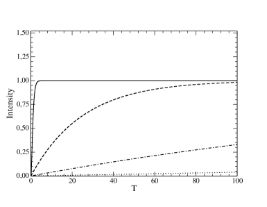
Figure 4: Light intensity as a function of dimensionless time $T=g_{0}t$ for the case that the excitons are initially in a number state $N_{b}=2$ for $g_{0}\tau_{0}=0.25$ (solid line), $g_{0}\tau_{0}=0.01$ (dashed line), $g_{0}\tau_{0}=0.001$ (dashed dotted line) and $g_{0}\tau_{0}=0.0001$ (dotted line). The intensity is in arbitrary units.

5 Conclusion

We studied a system of two linearly coupled oscillators and the effects of a phase fluctuating coupling. The model can be solved analytically and displays the weak-strong coupling transition. We show that this transition is a function of a dimensionless parameter $g_{0}\tau_{0}$ and occurs at $g_{0}\tau_{0}=0.25$. In the weak coupling regime we provide for an analytical expression for the damping parameter and compare with that of Ref. [4], in the context of exciton-polariton oscillations. The strong coupling regime leads to a “freezing” of the dynamics and may qualitatively provide for yet a third explanation for the self-trapping phenomenon in BEC (the first two given in Refs. [9, 11] and [14]).

References

References

- [1] A. J. Leggett, S. Chakravarty, A. T. Dorsey, M. P. A. Fisher, A. Garg, and W. Zweger, Rev. Mod. Phys. 59, 1 (1987); A. O. Caldeira and A. J. Leggett, Phys. Rev. A 31, 1059 (1985).
- [2] A. Rivas, A. D. K. Plato, S. F. Huelga and M. B. Plenio, New J. Phys. 12, 113032 (2010).
- [3] J. Jacobson, S. Pau, H. Cao, G. Björk and Y. Yamamoto, Phys. Rev. A 51, 2542 (1995).
- [4] S. Pau, G. Björk, J. Jacobson, H. Cao, and Y. Yamamato, Phys. Rev. B 51, 14437 (1995).
- [5] J. Bernu, S. Del glise, C. Sayrin, S. Kuhr, I. Dotsenko, M. Brune, J.M. Raimond, S. Haroche, Phys. Rev. Lett. 101, 180402 (2008).
- [6] A. R. Bosco de Magalhaes, R. Rossi, M. C. Nemes, Phys. Lett. A 375, 1724 (2011).
- [7] M. Albiez et al., Phys. Rev. Lett. 95, 010402 (2005).
- [8] G. Milburn et al., Phys. Rev. A 55, 4318 (1997).
- [9] A. Smerzi et al., Phys. Rev. Lett. 79, 4950 (1997).
- [10] J. Ruostekoski, D. Walls, Phys. Rev. A 58, R50 (1998).
- [11] F. Meier, W. Zwerger, Phys. Rev. A 64, 033610 (2001).
- [12] G. Kalosaka, A. R. Bishop, Phys. Rev. A 65, 043616 (2002).
- [13] G. Kalosaka et al., Phys. Rev. A 68, 023602 (2003).
- [14] A. N. Salgueiro et al., Eur. Phys. J. D 44, 537 (2007).
- [15] A. I. Burshtein and Yu S. Oseledchilk, Zh. Eksp. Teor. Fiz. 51 1071 (1966); (Engl. Transl., Sov. Phys.-. JETP 24 716 (1967)).
- [16] A. Joshi, J. Mod. Opt., 42(12), 2561 (1995).
- [17] E. A. Ospina. Processos Estocásticos na Interação da Luz com a Matéria. Dissertação de mestrado, UFMG, Belo Horizonte, Brazil, 2009.
- [18] W. H. Zurek, Phys. Rev. D 26, 1862 (1982) .
- [19] Y. Yamamoto, R. E. Slusher, Phys. Today 46, 66 (1993).
- [20] C. Weisbuch, M. Nishioka, A. Ishikawa, and Y. Arakawa, Phys. Rev. Lett. 69, 3314 (1992); R. Houdré, R. P. Stanley, U. Oesterle and M. Ilegems, Phys. Rev. B 49, 16761 (1994).
- [21] S. Schneider and G. J. Milburn, Phys. Rev. A 57, 3748 (1998).
- [22] S. Dyrting and G. J. Milburn, Quantum Semiclass. Opt. 8, 541 (1996).
- [23] D. M. Meekhof, C. Monroe, B. E. King, W. M. Itano, and D. J. Wineland, Phys. Rev. Lett. 76, 1796 (1996); 77, 2346(E) (1996).
- [24] S. Maniscalco, F. Francica, R.L. Zaffino, N. Lo Gullo, F. Plastina, Phys. Rev. Lett. 100, 090503 (2008).
- [25] J. G. Oliveira Jr., R. Rossi, M. C. Nemes, Phys. Rev. A 78, 044301 (2008).
- [26] S. Pascazio, M. Namiki, Phys. Rev. A 50, 4582 (1994).
- [27] Y. Khodorkovsky, G. Kurizki, A. Vardi, Phys. Rev. Lett. 100, 220403 (2008).
- [28] Y. Khodorkovsky, G. Kurizki, A. Vardi, Phys. Rev. A 80, 023609 (2009).