Semiclassical Cauchy Estimates and applications

1. Introduction

In this note, we study the solutions to semiclassical Schrödinger equations on a real analytic manifold $M$ of dimension $n>1$:

$$(-h^{2}\Delta_{g}+V(x)-E(h))u(h)=0,$$ (1.1)

where $V$ and $g$ are real-analytic function and metric on $M$, respectively and $E(h)\to E_{0}$ as $h\to 0$. We also consider more general differential operators and, when $M={\mathbb{R}}^{n}$, analytic pseudodifferential operators satisfying suitable ellipticity condition.

The analyticity of $V$ and of the metric $g$ imply that solutions are real analytic [12, Theorem 8.6.1, 9.5.1(for hyperfunctions)] and in particular Cauchy estimates hold:

$$\sup_{K}|\partial^{\alpha}u(x)|\leq C_{h}^{|\alpha|}|\alpha|^{|\alpha|},\ \ \forall\,K\Subset M,$$

for some constant $C_{h}$ depending on $h$. The semiclassical Cauchy estimate provides the following improvement:

$$\sup_{K}|\partial^{\alpha}u(x)|\leq h^{-\frac{n-1}{2}}C^{|\alpha|}(h^{-1}+|\alpha|)^{|\alpha|},\ \ \forall\,K\Subset M,$$ (1.2)

where $C$ depends only on $g$, $V$ and $K$.

The proof of (1.2) uses the FBI transform approach to analytic semiclassical theory developed by Sjöstrand [15] and Martinez [14]. It is presented in Section 2 that near every point the solution $u$ can be analytic continued to a holomorphic function in a uniform complex neighborhood. Moreover, the analytic continuation will grow at most exponentially in $h^{-1}$, which as we will see, is equivalent to the semiclassical version of the Cauchy estimates on the derivatives of $u$.

We should remark that for differential operators one can obtain estimates equivalent to (1.2) (see Proposition 2.2) by using Hörmander’s approach to analytic hypoellipticity and rescaling – see [5, Lemma 7.1]. In fact, we learned about this after proving (1.2) directly using the FBI transform and the study of the Donnelly-Fefferman paper [5] led to applications to the volume of nodal sets (zero set of $u(h)$) in the semiclassical setting. An illustration of the level sets of eigenfunctions is shown in Fig. 1: the zero sets occur in the regions where the eigenfunction is “small” and, in particular, are indistinguishable from the classically forbidden regions.

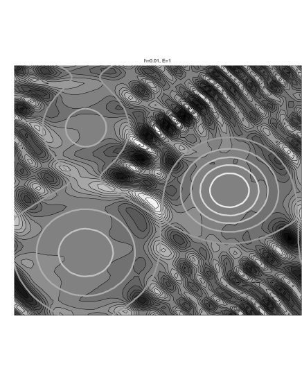
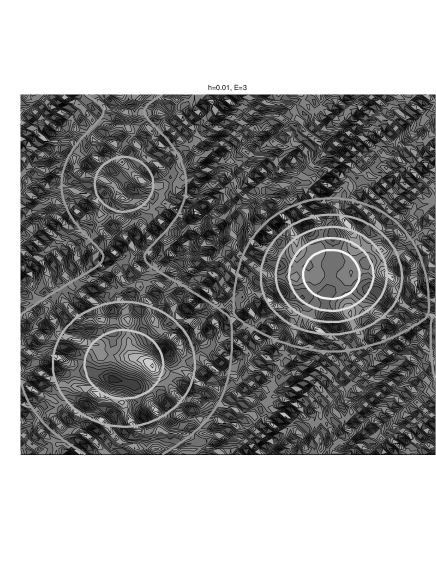
Figure 1. Level sets of eigenfunctions of $-h^{2}\Delta+V$ on a torus, $[0,1]\times[0,1]$ where $h=0.01$ and $V$ is a periodized sum of three bumps: $5e^{-10((x-0.75)^{2}+(y-0.5)^{2}))}+2e^{-10((x+0.25)^{2}+(y-0.75)^{2})}+3e^{-5((x+0.25)^{2}+(y+0.25)^{2})}$ (with level sets shown). In the first picture the energy level is close to $1$ and in the second, to $3$ so that the difference in classically forbidden regions is clearly visible.

Section 3 contains a proof of the doubling property of solutions to (1.1) where we allow the manifold and the potential to be merely smooth. This type of results have been proved in more general setting, e.g. [1] for $C^{1}$-potentials and are closely related to the unique continuation problems. There are two different ways to achieve such kind of results: the usual approach is through the Carleman-type estimates which establish a priori estimates with a weight; another approach was developed by Garofalo and Lin [7] based on a combination of geometric and variational ideas. We shall follow the usual approach.

Finally in Section 4, we study the vanishing property of solutions to (1.1). We shall show that the vanishing order of $u$ at a point is at most $Ch^{-1}$ and the nodal set of $u$, i.e. the set where $u$ vanishes, has $(n-1)$-dimensional Hausdorff measure $\sim h^{-1}$. When $V\equiv 0$, i.e. $u$ is eigenfunctions of the Laplacian operator on $M$ with eigenvalues $Eh^{-2}$, this is the analytic case of Yau’s conjecture [18] and is proved by Donnelly-Fefferman [5]. We shall follow their argument closely. In the smooth setting, this is still an open problem, exponential types of upper and lower bounds were first established by Hardt and Simon [10], see the notes [9] for a detailed study on nodal sets and [3], [16], [11], [17] for recent progress on Yau’s conjecture. Also see [19] for nodal sets of semiclassical Schrödinger operators in the smooth setting and [2] for the physics perspective.

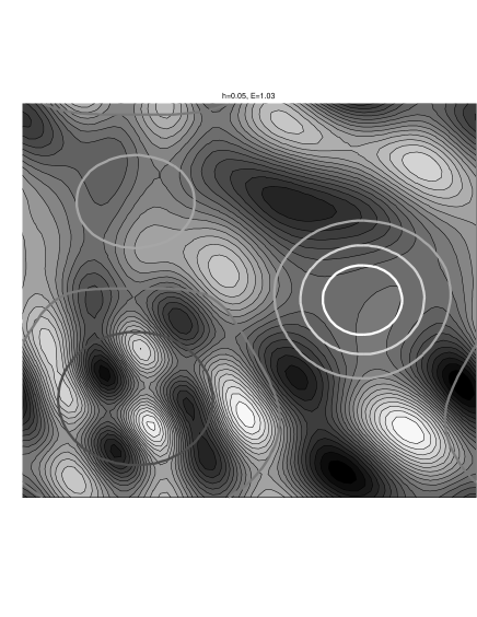
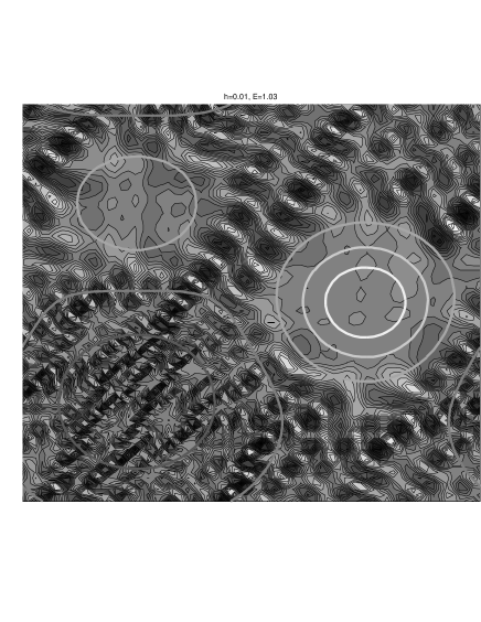
Figure 2. Level sets of eigenfunctions of $-h^{2}\Delta+V$ on a torus, $[0,1]\times[0,1]$ where $V$ is a periodized sum of two bumps and one well : $5e^{-10((x-0.75)^{2}+(y-0.5)^{2}))}+2e^{-10((x+0.25)^{2}+(y-0.75)^{2})}-3e^{-5((x+0.25)^{2}+(y+0.25)^{2})}$ (with level sets shown). The energy level is now fixed at $E=1$ but $h=0.05$ and $h=0.01$.

Acknowledgement

The author would like to thank Maciej Zworski for the encouragement and advice during the preparation of this paper. Thanks go also to Chris Wong for providing a MATLAB code for calculating eigenfunctions for Schrödinger operators on tori, and to the National Science Foundation for support in the Summer of 2012 under the grant DMS-1201417.

2. Semiclassical Cauchy Estimates and Analytic Continuation

2.1. Fourier-Bros-Iagolnitzer Transform

In this section we review some basic facts of Fourier-Bros-Iagolnitzer transform. For $h>0$, we define $T_{h}:\mathscr{S}^{\prime}(\mathbb{R}^{n})\to\mathscr{S}^{\prime}(\mathbb{R}^{2n})$ as

$$T_{h}u(x,\xi)=2^{-\frac{n}{2}}(\pi h)^{-\frac{3n}{4}}\int e^{\frac{i}{h}(x-y)\xi-\frac{1}{2h}(x-y)^{2}}u(y)dy.$$ (2.1)

In other words, $T_{h}u(x,\xi)=\langle\phi_{x,\xi},u\rangle_{\mathscr{S},\mathscr{S}^{\prime}}$ where $\phi_{x,\xi}$ is the so-called coherent state centered at $(x,\xi)$, so $T_{h}u(x,\xi)$ captures the microlocal property of $u$ at $(x,\xi)\in\mathbb{R}^{2n}$. We state some basic properties of the FBI transform:

(1) If $u\in\mathscr{S}^{\prime}(\mathbb{R}^{n})$, then $e^{\frac{\xi^{2}}{2h}}T_{h}u(x,\xi)$ is a holomorphic function of $z=x-i\xi\in\mathbb{C}^{n}$. In fact, $T_{h}(\mathscr{S}^{\prime}(\mathbb{R}^{n}))=\mathscr{S}^{\prime}(\mathbb{R}^{2n})\cap e^{-\frac{\xi^{2}}{2h}}\mathcal{H}(\mathbb{C}^{n}_{x-i\xi})$ where $\mathcal{H}(\mathbb{C}^{n}_{x-i\xi})$ is the space of entire functions on $\mathbb{C}^{n}$. This also shows $hD_{x}T_{h}u=(\xi+ihD_{\xi})T_{h}u$.

(2) For every $u\in\mathscr{S}^{\prime}(\mathbb{R}^{n})$, $u=T_{h}^{\ast}T_{h}u$ where $T_{h}^{\ast}$ is defined as

$$T_{h}^{\ast}v(y)=2^{-\frac{n}{2}}(\pi h)^{-\frac{3n}{4}}\int e^{-\frac{i}{h}(x-y)\xi-\frac{1}{2h}(x-y)^{2}}v(x,\xi)dxd\xi$$

(interpreted as an oscillatory integral with respect to $\xi$.)

(3) If $u\in L^{2}(\mathbb{R}^{n})$, then $T_{h}u\in L^{2}(\mathbb{R}^{2n})$ and $\|T_{h}u\|_{L^{2}(\mathbb{R}^{2n})}=\|u\|_{L^{2}(\mathbb{R}^{n})}$. Moreover, $T_{h}T_{h}^{\ast}$ is the orthogonal projection from $L^{2}(\mathbb{R}^{2n})$ onto $T_{h}(L^{2}(\mathbb{R}^{n}))=L^{2}(\mathbb{R}^{2n})\cap e^{-\frac{\xi^{2}}{2h}}\mathcal{H}(\mathbb{C}^{n}_{x-i\xi})$.

(4) Let $p\in S_{2n}(1)$, then $\tilde{p}(x,\xi,x^{\ast},\xi^{\ast})=p(x-\xi^{\ast},x^{\ast})$ belongs to $S_{4n}(1)$ and we have

$$T_{h}\circ p(x,hD_{x})=\tilde{p}(x,\xi,hD_{x},hD_{\xi})\circ T_{h}.$$

where $x^{\ast}$ and $\xi^{\ast}$ are the dual variables of $x$ and $\xi$ respectively. This formula is exact and $\tilde{p}$ does not depend on $\mu$ or which quantization we are using.

Bros and Iagolnitzer first use this type of transform to characterize analytic wavefront set: $(x_{0},\xi_{0})\in\operatorname{WF}_{a}(u)$ if and only if $T_{h}u(x,\xi)=O(e^{-\frac{c}{h}})$ uniformly in a neighborhood of $(x_{0},\xi_{0})$ for some $c>0$. In general, we can define FBI transform with a phase which “looks like” the standard phase above and an elliptic analytic symbol. All such FBI transform can be used to characterize analytic wavefront set, see [4], [15] and [20] for this general approach. For convenience, we shall only consider the standard FBI transform and the following modification.

Lemma 2.1 (Change of FBI by an analytic symbol).

Suppose $a=a(x,y,\xi)$ is an analytic symbol defined for $x,y\in\mathbb{C}^{n},\xi\in\mathbb{R}^{n}$ and is of tempered growth in $x,y,\xi$, $\mu>1$ fixed, then we define $T^{\prime}_{h}$ as

$$T^{\prime}_{h}u(x,\xi)=2^{-\frac{n}{2}}(\pi h)^{-\frac{3n}{4}}\int e^{\frac{i}{h}(x-y)\xi-\frac{\mu}{2h}(x-y)^{2}}a(x,y,\xi)u(y)dy$$ (2.2)

We have if $|T_{h}u(x,\xi)|=O(e^{-c/h})$ in a real neighborhood $U$ of $(x_{0},\xi_{0})$, then $|T_{h}^{\prime}u(x,\xi)|=O(e^{-c^{\prime}/h})$ in a neighborhood $V$ of $(x_{0},\xi_{0})$, where $c^{\prime}$ and $V$ only depends on $c$, the growth of $a$ and the size of $U$.

Proof.

We shall write $T_{h}^{\prime}u=T_{h}^{\prime}(T_{h}^{\ast}T_{h}u)=(T_{h}^{\prime}T_{h}^{\ast})T_{h}u$.

$$T_{h}^{\prime}u(x,\xi)=\iiint e^{\frac{i}{h}(x-y)\xi-\frac{\mu}{2h}(x-y)^{2}-\frac{i}{h}(\tilde{x}-y)\tilde{\xi}-\frac{1}{2h}(\tilde{x}-y)^{2}}a(x,y,\xi)T_{h}u(\tilde{x},\tilde{\xi})d\tilde{x}d\tilde{\xi}dy.$$

Therefore

$$T_{h}^{\prime}u(x,\xi)=\iint b(x,\xi,\tilde{x},\tilde{\xi})T_{h}u(\tilde{x},\tilde{\xi})d\tilde{x}d\tilde{\xi}$$ (2.3)

where

$$b(x,\xi,\tilde{x},\tilde{\xi})=e^{\frac{1}{\mu+1}\frac{i}{h}(x-\tilde{x})(\xi+\mu\tilde{\xi})-\frac{\mu}{\mu+1}\frac{1}{2h}(x-\tilde{x})^{2}-\frac{1}{\mu+1}\frac{1}{2h}(\xi-\tilde{\xi})^{2}}\int e^{-\frac{\mu+1}{2h}(y-\frac{\mu x+\tilde{x}}{\mu+1}+i\frac{\xi-\tilde{\xi}}{\mu+1})^{2}}a(x,y,\xi)dy$$

Now we change the contour to $y\mapsto y+\frac{\mu x+\tilde{x}}{\mu+1}-i\frac{\xi-\tilde{\xi}}{\mu+1}$,

$$b(x,\xi,\tilde{x},\tilde{\xi})=e^{\frac{1}{\mu+1}\frac{i}{h}(x-\tilde{x})(\xi+\mu\tilde{\xi})-\frac{\mu}{\mu+1}\frac{1}{2h}(x-\tilde{x})^{2}-\frac{1}{\mu+1}\frac{1}{2h}(\xi-\tilde{\xi})^{2}}\int e^{-\frac{\mu+1}{2h}y^{2}}a(x,y+\frac{\mu x+\tilde{x}}{\mu+1}-i\frac{\xi-\tilde{\xi}}{\mu+1},\xi)dy$$

and use the assumption that $a$ is of tempered growth in $x,y,\xi$, we have

$$|b(x,\xi,\tilde{x},\tilde{\xi})|\leqslant Ce^{-\frac{\delta}{h}(x-\tilde{x})^{2}-\frac{\delta}{h}(\xi-\tilde{\xi})^{2}}.$$

where $\delta,C$ depends only on the growth of $a$. Now the theorem follows easily from $\eqref{eq:chfbi}$ by separating the integral to two parts: $(\tilde{x},\tilde{\xi})$ close to $(x,\xi)$ and $(\tilde{x},\tilde{\xi})$ far away from $(x,\xi)$. ∎

2.2. Equivalence between Cauchy estimates and decay of the FBI transform

In this section, we prove the equivalence between the semiclassical Cauchy estimate and the uniform exponential decay for the FBI transform when $|\xi|$ is large. Comparing to [14], we use different parameters for the FBI transform and the function $u$ itself, so we can capture both the microlocal and semiclassical properties of $u$. The idea of the proof is similar to the proof of the fact the projection of analytic wavefront set is the analytic singular support, see [15].

Proposition 2.2.

Let $u=u(h),0<h\leqslant h_{0}$ be a family of function on a neighborhood $X$ of $x_{0}\in\mathbb{R}^{n}$ such that $\|u\|_{L^{\infty}(X)}=O(h^{-N})$. Then the following are equivalent:
(i) There exists an open neighborhood $V\subset\subset X$ of $x_{0}$ and constants $C_{0},C_{1},\delta>0$ such that for every $0<\tilde{h}\leqslant h\leqslant h_{0}$, $x\in V$ and $|\xi|\geqslant C_{0}$,

$$|T_{\tilde{h}}u(x,\xi,h)|\leqslant C_{1}e^{-\frac{\delta}{\tilde{h}}}\|u\|_{L^{\infty}}.$$ (2.4)

(ii) There exists a complex neighborhood $W\subset\subset X+i\mathbb{R}^{n}$ of $x_{0}$ and a constant $C,C_{2}>0$ such that $u(h)$ can be extended holomorphic to $W$ and

$$\sup_{W}|u(h)|\leqslant C_{2}e^{\frac{C}{h}}\|u\|_{L^{\infty}}.$$ (2.5)

(iii) There exists an open neighborhood $U\subset\subset X$ of $x_{0}$, there exists $C_{3}>0$ such that for all $x\in U$,

$$|(hD)^{\alpha}u(x)|\leqslant C_{3}^{|\alpha|}(1+h|\alpha|)^{|\alpha|}\|u\|_{L^{\infty}}.$$ (2.6)

Proof.

First we notice that all of the statements are local, so we can extend $u$ to functions on $\mathbb{R}^{n}$, say by setting $u=0$ outside $X$, or better, to a family of functions in $C_{0}^{\infty}$ since each condition implies that $u$ is smooth (in fact, analytic) near $x_{0}$. Also if (ii) is true, then by Hadamard’s three line theorem, there exists new constants $C,C_{2}>0$ such that

$$|u(z)|\leqslant C_{2}h^{-N}e^{\frac{C|\mathop{\rm Im}\nolimits z|}{h}}.$$ (2.7)

To prove that (ii) and (iii) are equivalent, we need the following elementary inequalities:

$$\forall t,s>0,(1+\frac{s}{t})^{t}\leqslant e^{s}\leqslant(1+\frac{s}{t})^{t+s}.$$ (2.8)

$$\forall\alpha\in\mathbb{N}^{n},(ne)^{-|\alpha|}|\alpha|^{|\alpha|}\leqslant\alpha!\leqslant|\alpha|^{|\alpha|}.$$ (2.9)

Proof of (ii)$\Rightarrow$(iii): We can find a real neighborhood $U\subset\subset X$ of $x_{0}$ and a constant $r_{0}>0$ such that for all $x\in U$, the polydisc $D(x,r_{0})\subset\subset W$, then by Cauchy’s inequality (see [13] Theorem 2.2.7.) on $D(x,r)$ we have for a new constant $C>0$,

$$|(hD)^{\alpha}u(x)|\leqslant Ch^{-N}e^{\frac{Cr}{h}}h^{|\alpha|}\alpha!r^{-|\alpha|},0<r\leqslant r_{0},x\in U.$$ (2.10)

Case 1: If $r_{0}\geqslant\frac{h|\alpha|}{C}$, then we take $r=\frac{h|\alpha|}{C}$ in (2.10) and get

$$|(hD)^{\alpha}u(x)|\leqslant Ch^{-N}e^{|\alpha|}\alpha!C^{|\alpha|}|\alpha|^{-|\alpha|}$$

Now by (2.9), we have for a new constant $C>0$,

$$|(hD)^{\alpha}u(x)|\leqslant C^{|\alpha|}h^{-N}.$$

This implies (2.6).

Case 2: If $r_{0}<\frac{h|\alpha|}{C}$, then we take $r=r_{0}$ in (2.10) and get

$$|(hD)^{\alpha}u(x)|\leqslant Ch^{-N}e^{\frac{Cr_{0}}{h}}h^{|\alpha|}\alpha!r_{0}^{-|\alpha|}$$

We use (2.8) for $s=Cr_{0},t=h|\alpha|$ and (2.9). Then

$$\begin{split}|(hD)^{\alpha}u(x)|&\leqslant Ch^{-N}(1+\frac{Cr_{0}}{h|\alpha|})^{\frac{Cr_{0}}{h}+|\alpha|}h^{|\alpha|}|\alpha|^{|\alpha|}r_{0}^{-|\alpha|}\\ &=Ch^{-N}(1+\frac{Cr_{0}}{h|\alpha|})^{\frac{Cr_{0}}{h}}(Cr_{0}+h|\alpha|)^{|\alpha|}r_{0}^{-|\alpha|}\end{split}$$

which also implies (2.6) by our assumption $\frac{Cr_{0}}{h}<|\alpha|$.

Proof of (iii)$\Rightarrow$(ii): For $\delta>0$ small enough, $B(x_{0},\delta)=\{|x-x_{0}|<\delta\}\subset U$, then for $x\in B(x_{0},\delta)$, by Taylor’s theorem,

$$u(x)=\sum_{0\leqslant|\alpha|\leqslant k-1}\frac{\partial^{\alpha}u(x_{0})}{\alpha!}(x-x_{0})^{\alpha}+R_{k}$$

where

$$R_{k}=\sum_{|\alpha|=k}\frac{1}{\alpha!}(x-x_{0})^{\alpha}\int_{0}^{1}k(1-t)^{k-1}\partial^{\alpha}u(x_{0}+t(x-x_{0}))dt$$

Therefore by (2.6),

$$|R_{k}|\leqslant\sum_{|\alpha|=k}\frac{1}{\alpha!}\delta^{k}C_{3}^{k}(1+hk)^{k}h^{-k}$$

We use (2.8) and (2.9) again to get

$$|R_{k}|\leqslant(k+1)^{n}(C_{3}ne\delta)^{k}(1+\frac{1}{hk})^{k}\leqslant e^{\frac{1}{h}}(k+1)^{n}(C_{3}ne\delta)^{k}$$

Therefore as long as $\delta<(C_{3}ne)^{-1}$, $R_{k}\to 0$ as $k\to\infty$, so $u$ is analytic on $B(x_{0},\delta)$. Now we can extend $u$ holomorphically to $W=\{z\in\mathbb{C}^{n}:|z-x_{0}|<\delta\}$ by

$$u(z)=\sum_{\alpha}\frac{\partial^{\alpha}u(x_{0})}{\alpha!}(z-x_{0})^{\alpha}.$$ (2.11)

Since

$$\left|\frac{\partial^{\alpha}u(x_{0})}{\alpha!}(z-x_{0})^{\alpha}\right|\leqslant\frac{C_{3}^{|\alpha|}(1+h|\alpha|)^{|\alpha|}}{h^{|\alpha|}\alpha!}\delta^{|\alpha|}.$$

We apply (2.8) for $s=1,t=h|\alpha|$ and (2.9) to get

$$\left|\frac{\partial^{\alpha}u(x_{0})}{\alpha!}(z-x_{0})^{\alpha}\right|\leqslant(C_{3}ne\delta)^{|\alpha|}(1+\frac{1}{h|\alpha|})^{|\alpha|}\leqslant(C_{3}ne\delta)^{|\alpha|}e^{\frac{1}{h}}.$$

Thus

$$|u(z)|\leqslant\sum_{\alpha}\left|\frac{\partial^{\alpha}u(x_{0})}{\alpha!}(z-x_{0})^{\alpha}\right|\leqslant e^{\frac{1}{h}}\sum_{\alpha}(C_{3}ne\delta)^{|\alpha|}.$$

which gives (2.5) since $\delta<(C_{3}ne)^{-1}$.

Now we turn to the proof of (i)$\Leftrightarrow$(ii). We use the same type of deformation of the integral contour as in the proof that the projection of analytic wavefront set is the analytic singular support (see [15]).
Proof of (ii)$\Rightarrow$(i): We have (2.7) for $z$ in a neighborhood of $x_{0}$, say $\{z=y+it:|y-x_{0}|<2r,|t|<r\}$. For $|x-x_{0}|<r$, in the formula of FBI transform (2.1),

$$T_{\tilde{h}}u(x,\xi,h)=2^{-\frac{n}{2}}(\pi\tilde{h})^{-\frac{3n}{4}}\int e^{\frac{i}{\tilde{h}}(x-y)\xi-\frac{1}{2\tilde{h}}(x-y)^{2}}u(y)dy,$$

we deform the contour to

$$\Gamma_{x}:y\mapsto z=y+i\epsilon\chi(y)\frac{\xi}{|\xi|}.$$ (2.12)

where $\chi\in C_{0}^{\infty}(\mathbb{R}^{n}),0\leqslant\chi\leqslant 1,\chi=1$ on $|y-x|<\frac{r}{2}$, $\operatorname{supp}\chi\subset\{|y-x|<r\}$ and $\epsilon\in(0,r)$. Then along $\Gamma_{x}$,

$$\left|e^{\frac{i}{\tilde{h}}(x-z)\xi-\frac{1}{2\tilde{h}}(x-z)^{2}}u(z)\right|\leqslant Ch^{-N}e^{\frac{C}{h}\epsilon\chi(y)-\frac{1}{\tilde{h}}\epsilon\chi(y)|\xi|+\frac{1}{2\tilde{h}}\epsilon^{2}\chi(y)^{2}-\frac{|x-y|^{2}}{2\tilde{h}}}.$$

Since

$$\frac{C}{h}\epsilon\chi(y)-\frac{1}{\tilde{h}}\epsilon\chi(y)|\xi|+\frac{1}{2\tilde{h}}\epsilon^{2}\chi(y)^{2}-\frac{|x-y|^{2}}{2\tilde{h}}\leqslant\frac{1}{\tilde{h}}\epsilon\chi(y)[C+\frac{\epsilon}{2}-|\xi|]-\frac{|x-y|^{2}}{2\tilde{h}}$$

we have if $|\xi|>C_{0}=C+\frac{\epsilon}{2}+\frac{\delta}{\epsilon}$,

$$\left|e^{\frac{i}{\tilde{h}}(x-z)\xi-\frac{1}{2\tilde{h}}(x-z)^{2}}u(z)\right|\leqslant\left\{\begin{array}[]{ll}Ch^{-N}e^{-\frac{\delta}{\tilde{h}}},&\text{ when }|y-x|<\frac{r}{2}\\ Ch^{-N}e^{-\frac{r^{2}}{8\tilde{h}}},&\text{ when }|y-x|\geqslant\frac{r}{2}\end{array}\right.$$

which shows (2.4).

Proof of (i)$\Rightarrow$(ii): We have

$$\delta(x)=(2\pi h)^{-n}\int e^{\frac{i}{h}x\xi}d\xi$$

in the sense of oscillatory integral. Following Lebeau, we deform to the complex contour

$$\tilde{\Gamma}_{x}:\xi\mapsto\zeta=\xi+\frac{i}{2}|\xi|x$$ (2.13)

Along $\tilde{\Gamma}_{x}$,

$$d\zeta=a(x,\xi)d\xi,a(x,\xi)=1+\frac{i}{2}\sum_{1}^{n}\frac{x_{j}\xi_{j}}{|\xi|}.$$

Therefore in the sense of oscillatory integral,

$$\delta(x)=(2\pi h)^{-n}\int e^{\frac{i}{h}x\xi-\frac{1}{2h}|\xi|x^{2}}a(x,\xi)d\xi.$$ (2.14)

Now we can write $u$ in the form of

$$u(x)=(2\pi h)^{-n}\iint e^{\frac{i}{h}(x-y)\xi-\frac{1}{2h}|\xi|(x-y)^{2}}a(x-y,\xi)u(y,h)dyd\xi.$$ (2.15)

Let

$$I(x,\xi,h)=\int e^{\frac{i}{h}(x-y)\xi-\frac{1}{2h}|\xi|(x-y)^{2}}a(x-y,\xi)u(y,h)dy,$$

We claim that

$$I(x+it,\xi,h)=O(e^{\frac{C}{h}-\frac{c|\xi|}{h}}),C,c>0$$ (2.16)

uniformly for $x+it$ in a complex neighborhood of $x_{0}$ and $0<h\leqslant h_{0}$. In fact,

$$I(x+it,\xi,h)=e^{-\frac{t\xi}{h}+\frac{t^{2}|\xi|}{2h}}\int e^{\frac{i}{h}(x-y)(\xi-|\xi|t)-\frac{1}{2h}|\xi|(x-y)^{2}}a(x+it-y,\xi)u(y)dy$$ (2.17)

It is easy to see when $|\xi|<C^{\prime}$, $I(x+it,\xi,h)=O(e^{\frac{C}{h}})$, so we have (2.16). Now we assume $|\xi|>C^{\prime}$ where $C^{\prime}$ we shall choose to be large later, then since $|t|<\epsilon$,

$$(1-\epsilon)|\xi|<|\xi-|\xi|t|<(1+\epsilon)|\xi|.$$

Let $\tilde{h}=\frac{\mu h}{|\xi|},\mu$ large and fixed later, then we can rewrite (2.17) as

$$I(x+it,\xi,h)=e^{-\frac{t\xi}{h}+\frac{t^{2}|\xi|}{2h}}\int e^{\frac{i}{\tilde{h}}(x-y)\cdot(\frac{\tilde{h}}{h}(\xi-|\xi|t))-\frac{\mu}{2\tilde{h}}(x-y)^{2}}a(x+it-y,\xi)u(y)dy$$

Now we choose $C^{\prime}>\mu>C_{0}(1-\epsilon)^{-1}$, then $\tilde{h}\leqslant h$ and

$$\left|\frac{\tilde{h}}{h}(\xi-|\xi|t)\right|=\mu\frac{|\xi-|\xi|t|}{|\xi|}\geqslant(1-\delta)\mu>C_{0}$$

By Lemma 2.1 (we notice that $y\mapsto a(x+it-y,\xi)$ has uniform tempered growth when $|t|$ is small) and (2.4), we have uniform exponential decay for the integral in (2.17) when $x+it$ is in a small complex neighborhood of $x_{0}$, and $|\xi|>C^{\prime}$,

$$I(x+it,\xi,h)\leqslant Ce^{-\frac{t\xi}{h}+\frac{t^{2}|\xi|}{2h}}e^{-\frac{\delta^{\prime}}{\tilde{h}}}\leqslant Ce^{-\frac{c|\xi|}{h}}.$$

if we assume $|t|<\epsilon$ is small enough. This finishes the proof of (2.16).

Now we can extend $u$ holomorphically to a complex neighborhood of $x_{0}$ simply by

$$u(z)=(2\pi h)^{-n}\int I(z,\xi,h)d\xi.$$ (2.18)

since $I(z,\xi,h)$ is holomorphic and the integral is uniformly convergent. Furthermore,

$$|u(z)|\leqslant C(2\pi h)^{-n}\int e^{\frac{C}{h}-\frac{c|\xi|}{h}}d\xi\leqslant C_{2}e^{\frac{C}{h}}.$$ (2.19)

which gives (2.5). ∎

Remark 2.3.

Since $e^{\frac{\xi^{2}}{2\tilde{h}}}T_{\tilde{h}}u(x,\xi;h)$ is holomorphic, we can replace condition (i) by the exponential decay of local $L^{2}$-norm of $T_{\tilde{h}}u(h)$.

2.3. Agmon estimates for the FBI transform

We shall follow the approach in [14]. First we recall the following theorem of microlocal exponential estimate from [14, Corollary 3.5.3, $f=1$]:

Theorem 2.4.

Suppose $p\in S_{2n}(1)$ can be extended holomorphically to

$$\Sigma(a)=\{(x,\xi)\in\mathbb{C}^{2n}:|\mathop{\rm Im}\nolimits x|<a,|\mathop{\rm Im}\nolimits\xi|<a\}$$

such that

$$\forall\alpha\in\mathbb{N}^{2n},\partial^{\alpha}p=O(1),\text{ uniformly in }\Sigma(a).$$

Assume also that the real-valued function $\psi\in S_{2n}(1)$ satisfies

$$\sup_{\mathbb{R}^{2n}}|\nabla_{x}\psi|<a,\sup_{\mathbb{R}^{2n}}|\nabla_{\xi}\psi|<a.$$

Then

$$\|e^{\psi/h}T_{h}P(x,hD)u\|^{2}=\|p(x-2\partial_{z}\psi,\xi+2i\partial_{z}\psi)e^{\psi/h}T_{h}u\|^{2}+O(h)\|e^{\psi/h}T_{h}u\|^{2}$$

uniformly for $u\in L^{2}(\mathbb{R}^{n})$, $h>0$ small enough. Here $\partial_{z}=\frac{1}{2}(\partial_{x}+i\partial_{\xi})$ is the holomorphic derivative with respect to $z=x-i\xi$.

Remark 2.5.

From the argument in [14], we can also see that this estimate only depends on the seminorms of $p$ and $\psi$ in $S_{2n}(1)$. In other words, if $p$ and $\psi$ varies in a way such that every $\sup\limits_{\Sigma(a,b)}|\partial^{\alpha}p|$ and $\sup\limits_{\mathbb{R}^{2n}}|\partial^{\alpha}\psi|$ is uniformly bounded, then the estimate is uniform in $p$ and $\psi$. Furthermore, we only need that $p$ can be extended holomorphically to the set $\{(y,\eta)\in\mathbb{C}^{2n}:\exists(x,\xi)\in\operatorname{supp}\psi,|y-x|<\sup|\nabla\psi|,|\eta-\xi|<\sup|\nabla\psi|\}$. Also here $P(x,hD)$ can be replaced by any quantization as in [14],[20].

Now we consider a semiclassical differential operator $P=P(x,hD_{x})$ of order $m$ with analytic coefficients, defined in a neighborhood $X$ of $x_{0}$. We assume the symbol

$$p(x,\xi;h)=\sum_{|\alpha|\leqslant m}a_{\alpha}(x;h)\xi^{\alpha}$$

can be extended holomorphically to a fixed complex neighborhood

$$\Sigma_{\delta}=\{(x,\xi)\in\mathbb{C}^{n}\times\mathbb{C}^{n}:|\mathop{\rm Re}\nolimits x-x_{0}|<\delta,|\mathop{\rm Im}\nolimits x|<\delta,|\mathop{\rm Im}\nolimits\xi|<\delta\}$$

and also that $P$ is classically elliptic in $\Sigma_{\delta}$, in the sense that the principal symbol

$$p_{0}(x,\xi)=\sum_{|\alpha|=m}a_{\alpha}\xi^{\alpha}$$

satisfies

$$|p_{0}(x,\xi)|\geqslant\frac{1}{C_{0}}\langle\mathop{\rm Re}\nolimits\xi\rangle^{m},\text{ for }(x,\xi)\in\Sigma_{\delta},|\mathop{\rm Re}\nolimits\xi|>C$$

Theorem 2.6.

Let $P$ be as above and assume $\{u(h)\}_{0<h\leqslant h_{0}}$ is a family of functions defined in $X$ such that

$$P(x,hD_{x})u(h)=0\text{ in }X$$

and

$$\|u(h)\|_{L^{2}(X)}\leqslant Ch^{-N}$$

Then there exists an open neighborhood $U\subset\subset X$ of $x_{0}$, such that for all $x\in U$,

$$|(hD)^{\alpha}u(x)|\leqslant C^{|\alpha|}(1+h|\alpha|)^{|\alpha|}\|u(h)\|_{L^{\infty}}.$$ (2.20)

Remark 2.7.

Also by the standard semiclassical elliptic estimates, (e.g. [20, Lemma 7.10]), we know $\|u\|_{L^{\infty}}\leqslant Ch^{-n/2}\|u\|_{L^{2}}$. So we also have $\|u(h)\|_{L^{\infty}}\leqslant Ch^{-M}$.

Proof.

First for $0<\tilde{h}\leqslant h$, we write

$$\tilde{P}(x,\tilde{h}D_{x})=(\tilde{h}/h)^{m}\chi_{1}(x)P(x,hD_{x})$$

so

$$\tilde{p}(x,\xi)=\sum_{|\alpha|\leqslant m}(\tilde{h}/h)^{m-|\alpha|}\chi_{1}(x)a_{\alpha}(x;h)\xi^{\alpha}$$

where $\chi_{1}\in C_{0}^{\infty}(\mathbb{R}^{n})$ is a cut-off function satisfying $\chi_{1}(x)=1$ for $|x-x_{0}|<\frac{\delta}{4}$; 0 for $|x-x_{0}|>\frac{\delta}{2}$. Therefore $\tilde{p}(x,\xi)$ can still be extended holomorphically to $\Sigma_{\frac{\delta}{4}}$ and classically elliptic in $\Sigma_{\frac{\delta}{4}}$. Now let $Q=\langle\tilde{h}D_{x}\rangle^{-m}\circ\tilde{P}(x,\tilde{h}D_{x})$, then we can write $Q(x,\tilde{h}D_{x})=\operatorname{Op}_{\tilde{h}}^{1}(q)$ where

$$q(y,\xi)=\langle\xi\rangle^{-m}\sum_{|\alpha|\leqslant m}\sum_{\beta\leqslant\alpha}(\tilde{h}D_{y})^{\beta}(\chi_{1}(y)a_{\alpha}(y;h))(-\xi)^{\alpha-\beta}.$$

In fact,

$$Qv=(2\pi\tilde{h})^{-n}\iint e^{\frac{i}{h}(x-y)\xi}\langle\xi\rangle^{-m}(\tilde{P}v)(y)dyd\xi=(2\pi\tilde{h})^{-n}\iint e^{\frac{i}{h}(x-y)\xi}q(y,\xi)v(y)dyd\xi.$$

Therefore $q$ can also be extended holomorphically to $\Sigma_{\frac{\delta}{4}}$ and

$$|\partial^{\alpha}q|=O_{\alpha}(1),\text{ in }\Sigma_{\frac{\delta}{4}}.$$

Furthermore $q$ is elliptic in $\Sigma_{\frac{\delta}{3}}$ and thus for $\tilde{h}$ small,

$$|q(x,\xi)|\geqslant\frac{1}{C},\text{ for }(x,\xi)\in\Sigma_{\frac{\delta}{4}},|\xi|>C_{0}.$$

Now let $v(x)=\chi_{2}(x)u(x)$, where $\chi_{2}(x)\in C_{0}^{\infty}(\mathbb{R}^{n})$ is a cut-off function satisfying $0\leqslant\chi_{2}\leqslant 1$, $\chi_{2}(x)=1$ for $|x-x_{0}|<\frac{\delta}{2}$; 0 for $|x-x_{0}|>\frac{3\delta}{4}$. Therefore $v\in L^{2}(\mathbb{R}^{n})$ and

$$Qv=0$$

$$\|v\|_{L^{2}(\mathbb{R}^{n})}\leqslant\|u\|_{L^{2}(X)}\leqslant Ch^{-N}.$$

Now we choose $\psi=\psi(x,\xi)\in S_{2n}(1)$ such that $\operatorname{supp}\psi\subset U_{1}=\{|x-x_{0}|<\frac{\delta}{8},|\xi|>2C_{0}\}$ and $\psi=c>0$ on $U_{2}=\{|x-x_{0}|<\frac{\delta}{16},|\xi|>3C_{0}\}$ and $\sup_{\mathbb{R}^{2n}}|\nabla_{(x,\xi)}\psi|<\frac{\delta}{16}$. Then if $(x,\xi)\in\operatorname{supp}\psi$, then for any $(y,\eta)\in\mathbb{C}^{2n}$ satisfying $|y-x|<\frac{\delta}{16},|\eta-\xi|<\frac{\delta}{16}$, we have $(y,\eta)\in\Sigma_{\frac{\delta}{4}}$. This allows us to apply the microlocal exponential estimate for $\psi$ and $q$:

$$0=\|e^{\psi/\tilde{h}}T_{\tilde{h}}Qv\|^{2}=\|q(x-2\partial_{z}\psi,\xi+2i\partial_{z}\psi)e^{\psi/\tilde{h}}T_{\tilde{h}}v\|^{2}+O(\tilde{h})\|e^{\psi/\tilde{h}}T_{\tilde{h}}v\|^{2}$$

Therefore

$$\|q(x-2\partial_{z}\psi,\xi+2i\partial_{z}\psi)e^{\psi/\tilde{h}}T_{\tilde{h}}v\|_{L^{2}(U_{1})}^{2}=O(\tilde{h})\|e^{\psi/{\tilde{h}}}T_{\tilde{h}}v\|^{2}$$

For $(x,\xi)\in U_{1}$, $(x-2\partial_{z}\psi,\xi+2i\partial_{z}\psi)\in\Sigma_{\frac{\delta}{4}}$ and $|\mathop{\rm Re}\nolimits(\xi+2i\partial_{z}\psi)|\geqslant 2C_{0}-\frac{\delta}{16}>C_{0}$, so

$$|q(x-2\partial_{z}\psi,\xi+2i\partial_{z}\psi)|\geqslant\frac{1}{C}.$$

Therefore

$$\|e^{\psi/\tilde{h}}T_{\tilde{h}}v\|_{L^{2}(U_{1})}^{2}=O(\tilde{h})\|e^{\psi/{\tilde{h}}}T_{\tilde{h}}v\|^{2}$$

When $\tilde{h}$ is small, we have

$$\|e^{\psi/\tilde{h}}T_{\tilde{h}}v\|_{L^{2}(U_{1})}^{2}=O(\tilde{h})\|e^{\psi/{\tilde{h}}}T_{\tilde{h}}v\|^{2}_{L^{2}(\mathbb{R}^{2n}\setminus U_{1})}$$

Since $\psi=0$ outside $U_{1}$, we have

$$\|e^{\psi/\tilde{h}}T_{\tilde{h}}v\|_{L^{2}(U_{1})}^{2}\leqslant C\tilde{h}\|T_{\tilde{h}}v\|^{2}_{L^{2}(\mathbb{R}^{2n}\setminus U_{1})}\leqslant C\tilde{h}\|T_{\tilde{h}}v\|^{2}=C\tilde{h}\|v\|^{2}\leqslant C\tilde{h}\|u\|^{2}.$$

Since $\psi=c>0$ on $U_{2}\subset U_{1}$,

$$\|T_{\tilde{h}}v\|_{L^{2}(U_{2})}\leqslant Ce^{-\frac{c}{\tilde{h}}}\|u\|^{2}.$$

Now by Proposition 2.2 and the remark after it, we can conclude the proof of (2.20). ∎

Remark 2.8.

The same argument can also be applied to elliptic pseudodifferential operators on $\mathbb{R}^{n}$ with symbol

$$p(x,\xi;h)\sim\sum_{j=0}^{\infty}a_{m}(x,\xi/|\xi|;h)|\xi|^{m-j}$$ (2.21)

which can be extended holomorphically to $\Sigma(a)$ for some $a>0$ and is classically elliptic in $\Sigma(a)$. In this case, we do not need any cut-off function and the weight function $\psi$ can be chosen to only depend on $\xi$. Then the solutions of $P(x,hD_{x})u(h)=0$ in $\mathbb{R}^{n}$ also satisfies the semiclassical Cauchy estimates (2.20).

3. Doubling property

In this section, we use a Carleman-type estimate to prove the so-called doubling property of solutions of semiclassical Schrodinger equations on a compact Riemannian manifold. We do not assume the analyticity of either the manifold or the potential. See [1] for a general setting where the potential is only assumed to be $C^{1}$. From now on, for simplicity, we shall use $\|u\|_{U}$ to represent the $L^{2}$-norm of the function $u$ in the set $U$.

Theorem 3.1.

Suppose $(M,g)$ is a compact Riemannian manifold, $V:M\to\mathbb{R}$ is a smooth function. Let $P(h)=-h^{2}\Delta_{g}+V(x)$ and $P(h)u(h)=E(h)u(h)$ where $E(h)\to E_{0}$ as $h\to 0$, then
(i) (Tunneling) For every $r>0$, there exists $c=c(r)>0$ depending on $r$ (and $(M,g),V$) such that

$$\|u\|_{L^{2}(B(p,r))}\geqslant e^{-c(r)/h}\|u\|_{L^{2}(M)}$$ (3.1)

for every $p\in M$, $0<h<h_{0}$.
(ii) (Doubling Property) There exists $c_{0}>0$ depending only on $(M,g)$ and $V$ and such that for every $c_{1}>0$,

$$\|u\|_{L^{2}(B(p,r))}\geqslant e^{-c_{0}/h}\|u\|_{L^{2}(B(p,2r))}$$ (3.2)

uniformly for $p\in M,r>c_{1}h$ and $0<h<h_{1}$.

Remark 3.2.

We can remove the condition $r>c_{1}h$ in part (ii) by carefully constructing a weight involving logarithmic terms near the origin in Carleman estimates. For the details, see [1]. For our purpose, the weak version above will be sufficient. From now on, in this section, every constant will depend on $(M,g)$ and $V$, but we shall not write it out explicitly.

3.1. Carleman estimates

We start by writing the equation in the local coordinates. Let $r_{1}$ be the injective radius of $M$, then for any $p\in M$, we write $P(h)u(h)=0$ on $B(p,r_{1})$ in the normal geodesic coordinates centered at $p$ still as

$$[-h^{2}\Delta_{g}+V(x)-E]u=0,x\in B(0,r_{1}).$$ (3.3)

Let $p=|\xi|^{2}_{g}+V(x)-E$ be the symbol of $P=-h^{2}\Delta_{g}+V(x)-E$. We wish to conjugate $P$ by a weight $e^{\varphi/h}$ to get an operator $P_{\varphi}=e^{\varphi/h}Pe^{-\varphi/h}$ whose symbol $p_{\varphi}=|\xi+i\partial\varphi(x)|^{2}_{g(x)}+V(x)-E$ satisfies Hörmander’s hypoelliptic condition:

$$\text{ if }p_{\varphi}=0,\text{ then }\frac{i}{2}\{p_{\varphi},\bar{p}_{\varphi}\}=\{\mathop{\rm Re}\nolimits p_{\varphi},\mathop{\rm Im}\nolimits p_{\varphi}\}>0.$$ (3.4)

on $B(0,R)\setminus B(0,r)$. Here $\{\cdot,\cdot\}$ denotes the Poisson bracket.

Since

$$\mathop{\rm Re}\nolimits p_{\varphi}=|\xi|^{2}_{g}-|\partial\varphi|^{2}_{g}+V-E,\mathop{\rm Im}\nolimits p_{\varphi}=2\langle\xi,\partial\varphi\rangle_{g}.$$

We have

$$\begin{split}\{\mathop{\rm Re}\nolimits p_{\varphi},\mathop{\rm Im}\nolimits p_{\varphi}\}=&\langle\partial_{\xi}(\mathop{\rm Re}\nolimits p_{\varphi}),\partial_{x}(\mathop{\rm Im}\nolimits p_{\varphi})\rangle-\langle\partial_{x}(\mathop{\rm Re}\nolimits p_{\varphi}),\partial_{\xi}(\mathop{\rm Im}\nolimits p_{\varphi})\rangle\\ =&4\langle g\xi,\partial^{2}\varphi g\xi\rangle+4\langle g\partial\varphi,\partial^{2}\varphi g\partial\varphi\rangle-2\langle g\partial\varphi,\partial V\rangle\\ &+4\langle g\xi,\langle\xi,\partial\varphi\rangle_{\partial g}\rangle-2\langle g\partial\varphi,|\xi|^{2}_{\partial g}-|\partial\varphi|^{2}_{\partial g}\rangle\end{split}$$

We set $\varphi=\tau e^{\mu\psi}$, where $\tau,\mu\geqslant 1$ is a large constant to be chosen later. Then

$$\partial\varphi=\tau\mu e^{\mu\psi}\partial\psi,\partial^{2}\varphi=\tau e^{\mu\psi}(\mu^{2}\partial\psi\otimes\partial\psi+\mu\partial^{2}\psi).$$

Therefore

$$\begin{split}\frac{i}{2}\{p_{\varphi},\bar{p}_{\varphi}\}=&\;4\tau\mu^{2}e^{\mu\psi}\langle g\xi,\partial\psi\rangle^{2}+4\tau\mu e^{\mu\psi}\langle g\xi,\partial^{2}\psi g\xi\rangle\\ &+4\tau^{3}\mu^{4}e^{3\mu\psi}\langle\partial\psi,g\partial\psi\rangle^{2}+4\tau^{3}\mu^{3}e^{3\mu\psi}\langle g\partial\psi,\partial^{2}\psi g\partial\psi\rangle\\ &-2\tau\mu e^{\mu\psi}\langle g\partial\psi,\partial V\rangle+4\tau\mu e^{\mu\psi}\langle g\xi,\langle\xi,\partial\psi\rangle_{\partial g}\rangle\\ &-2\tau\mu e^{\mu\psi}\langle g\partial\psi,|\xi|^{2}_{\partial g}\rangle+2\tau^{3}\mu^{3}e^{3\mu\psi}\langle g\partial\psi,|\partial\psi|^{2}_{\partial g}\rangle\end{split}$$

When $\mathop{\rm Re}\nolimits p_{\varphi}=\mathop{\rm Im}\nolimits p_{\varphi}=0$, we have

$$|\xi|^{2}_{g}=|\partial_{\varphi}|_{g}^{2}+V(x)-E=\tau^{2}\mu^{2}e^{2\mu\psi}|\partial\psi|_{g}^{2}+V-E$$

$$\langle\xi,\partial\varphi\rangle_{g}=2\tau\mu e^{\mu\psi}\langle g\xi,\partial\psi\rangle=0$$

thus

$$\xi=\tau\mu e^{\mu\psi}|\partial\psi|_{g}\eta,\text{ where }C_{1}^{-1}\leqslant|\eta|\leqslant C_{1}.$$

We shall choose $\psi$ to be a radial and radially decreasing function which equals to $A-|x|$ on $B(0,R)\setminus B(0,r)$ so that

$$\psi\geqslant 1,C_{2}^{-1}\leqslant|\partial\psi|_{g}\leqslant C_{2}\text{ and }|\partial^{2}\psi|\leqslant C_{2}\text{ on }B(0,R)\setminus B(0,r)$$

Hence

$$\frac{i}{2}\{p_{\varphi},\bar{p}_{\varphi}\}\geqslant 4\tau^{3}\mu^{4}e^{3\mu\psi}[|\partial\psi|_{g}^{4}-C_{3}\mu^{-1}]\geqslant C_{4}\tau^{-1}e^{-\mu\psi}\langle\psi\rangle^{4}$$

where $C_{3},C_{4}$ is a constant depending only on $\psi$ when $\mu$ and $\tau$ are large depending on $\psi$. Now we can prove the basic Carleman estimate:

Lemma 3.3.

For any $v\in C_{0}^{\infty}(B(0,R)\setminus B(0,r))$,

$$C_{5}\tau^{\frac{1}{2}}\|P_{\varphi}v\|\geqslant h^{\frac{1}{2}}\|v\|_{H_{h}^{2}}.$$ (3.5)

where $C_{5}$ is a constant only depending on $\mu,\psi$.

Proof.

The proof is based on the standard commutator argument. First,

$$\begin{split}\|P_{\varphi}v\|^{2}=&\langle P_{\varphi}v,P_{\varphi}v\rangle=\langle P_{\varphi}^{\ast}P_{\varphi}v,v\rangle\\ =&\langle P_{\varphi}^{\ast}P_{\varphi}v,v\rangle+\langle[P_{\varphi}^{\ast},P_{\varphi}]v,v\rangle=\|P_{\varphi}^{\ast}v\|^{2}+\langle[P_{\varphi}^{\ast},P_{\varphi}]v,v\rangle.\end{split}$$

For any $M>1$ and $h$ small enough, this implies

$$\begin{split}\|P_{\varphi}v\|^{2}&\geqslant Mh\|P_{\varphi}^{\ast}v\|^{2}+\langle[P_{\varphi}^{\ast},P_{\varphi}]v,v\rangle\\ &=h\langle\operatorname{Op}_{h}(M|p_{\varphi}|^{2}+i\{p_{\varphi},\bar{p}_{\varphi}\})u,u\rangle-O(h^{2})\|u\|_{H_{h}^{2}}\end{split}$$

From the construction above, we can find $M$ large enough so that

$$M|p_{\varphi}|^{2}+i\{p_{\varphi},\bar{p}_{\varphi}\}\geqslant C_{6}\tau^{-1}\langle\xi\rangle^{4}$$

where $C_{6}$ is a constant only depending on $\mu,\psi$. Now we can use the sharp Gårding’s inequality to conclude the lemma. ∎

Now we prove a Carleman estimate on different shells.

Proposition 3.4 (Carleman estimate on shells).

Let $\varphi$ be as above, we have the following estimate for solutions $u$ to the equation (3.3)

$$\begin{split}\|e^{\varphi/h}u\|_{B(0,\frac{R}{2})\setminus B(0,2r)}\leqslant&\;C_{7}\tau^{\frac{1}{2}}[R^{-2}e^{\varphi(\frac{R}{2})/h}\|u\|_{B(0,R)\setminus B(0,\frac{R}{2})}\\ &\;\;\;\;\;+r^{-2}e^{\varphi(2r)/h}\|u\|_{B(0,2r)\setminus B(0,r)}].\end{split}$$ (3.6)

where $0<8r<R<r_{1}$, $C_{7}>0$ only depends on $\mu,\psi$.

Proof.

We shall take $v=e^{\varphi/h}\chi u$ in (3.5) where $\chi$ is a function supported in $C_{0}^{\infty}(B(0,R)\setminus B(0,r))$, such that $\chi\equiv 1$ on $B(0,\frac{R}{2})\setminus B(0,2r)$, and

$$|\nabla\chi|\leqslant Cr^{-1},|\nabla^{2}\chi|\leqslant Cr^{-2}.$$

Then

$$\|v\|=\|e^{\varphi/h}\chi u\|\geqslant\|e^{\varphi/h}u\|_{B(0,\frac{R}{2})\setminus B(0,2r)},$$

and

$$\|P_{\varphi}v\|=\|e^{\varphi/h}P(\chi u)\|=\|e^{\varphi/h}[P,\chi]u\|$$

where $[P,\chi]=\langle a,hD\rangle+b$ is a first order differential operator supported on $\operatorname{supp}\nabla\chi\subset(B(0,R)\setminus B(0,\frac{R}{2}))\cup(B(0,2r)\setminus B(0,r))$ with coefficients $a=O(hr^{-1}),b=O(h^{2}r^{-2})$ on $B(0,2r)\setminus B(0,r)$ and with $r$ replaced by $R$ on $B(0,R)\setminus B(0,\frac{R}{2})$. Therefore by standard elliptic estimates (e.g. [20, Chapter 7]), we have

$$\begin{split}\|P_{\varphi}v\|\leqslant&\;C_{8}[e^{\varphi(\frac{R}{2})/h}\|u\|_{H_{h}^{1}(B(0,R)\setminus B(0,\frac{R}{2}))}+e^{\varphi(2r)/h}\|u\|_{H_{h}^{1}(B(0,2r)\setminus B(0,r))}]\\ \leqslant&\;C_{9}[R^{-2}h^{2}e^{\varphi(\frac{R}{2})/h}\|u\|_{B(0,R)\setminus B(0,\frac{R}{2})}+r^{-2}h^{2}e^{\varphi(r)/h}\|u\|_{B(0,2r)\setminus B(0,r)}].\end{split}$$

which finishes the proof. ∎

3.2. Proof of Theorem 3.1

We shall use 3.4 to prove Theorem 3.1. The tunneling estimate follows from the standard overlapping chains of balls argument introduced by Donnelly and Fefferman [5] while the doubling property is a corollary of the tunneling and the Carleman estimates on shells.

Proof of 3.1.

Without loss of generality, we can assume $\|u\|_{M}=1$ and we only need to prove 3.1 for $r<\frac{1}{100}r_{1}$. We shall fix $\tau$ large in the expression of $\varphi$ and replace $r$ by $\frac{r}{4}$ and take $R=32r$ in Proposition 3.4. Then we get

$$e^{\varphi(2r)/h}\|u\|_{B(x,2r)\setminus B(x,r)}\leqslant C_{10}[e^{\varphi(4r)/h}\|u\|_{B(x,8r)\setminus B(x,4r)}+e^{\varphi(\frac{r}{4})/h}\|u\|_{B(0,\frac{r}{2})\setminus B(0,\frac{r}{4})}]$$ (3.7)

for any $x\in M$. It is obvious that there exists a point $q\in M$ such that

$$\|u\|_{B(q,r)}\geqslant cr^{-n}\geqslant e^{-A_{0}/h}.$$

For any $p\in M$, we can find a sequence $x_{0}=q,x_{1},\ldots,x_{m}=p$ such that $d(x_{j},x_{j+1})<r$ and $m\leqslant C_{11}r^{-1}$. We shall prove by induction that there exists $A_{j}>0,h_{j}>0$ only depends on $r$ such that for $0<h<h_{j}$

$$\|u\|_{B(x_{j},r)}\geqslant e^{-A_{j}/h}.$$ (3.8)

We already know this is true for $j=0$. Suppose this is true for $j$, then for $j+1$, since $B(x_{j},r)\subset B(x_{j+1},2r)$, either

$$\|u\|_{B(x_{j+1},r)}\geqslant e^{-(A_{j}+1)/h}$$

or

$$\|u\|_{B(x_{j+1},2r)\setminus B(x_{j+1},r)}\geqslant e^{-(A_{j}+1)/h}.$$

For the first case, there is nothing to prove, for the later, we let $x=x_{j+1}$ in (3.7) to get

$$\|u\|_{B(0,\frac{r}{2})\setminus B(0,\frac{r}{4})}\geqslant e^{-\varphi(\frac{r}{4})/h}[C_{12}^{-1}h^{-\frac{3}{2}}e^{\varphi(2r)/h}e^{-(A_{j}+1)/h}-e^{\varphi(4r)/h}].$$ (3.9)

We only need to choose $\mu$ and $A$ large enough in the expression of $\varphi$ so that $\varphi(2r)-A_{j}-1>\varphi(4r)$ to get (3.8). Now since $m$ is bounded, we get the desired tunneling estimates 3.1. ∎

Proof of (3.2).

Again, we only need to prove (3.2) for $r\in(c_{1}h,\frac{r_{1}}{100})$. Now we shall fix $R=\frac{r_{1}}{2}$ in Proposition 3.4 and replace $r$ by $\frac{r}{2}$, then for any $p\in M$,

$$\begin{split}&e^{\varphi(\frac{R}{4})/h}\|u\|_{B(p,\frac{R}{4})\setminus B(p,\frac{R}{8})}+e^{\varphi(2r)/h}\|u\|_{B(p,2r)\setminus B(p,r)}\\ \leqslant&\;C_{13}\tau^{\frac{1}{2}}[e^{\varphi(\frac{R}{2})/h}\|u\|_{B(p,R)\setminus B(p,\frac{R}{2})}+h^{-2}e^{\varphi(\frac{r}{2})/h}\|u\|_{B(p,r)\setminus B(p,\frac{r}{2})}].\end{split}$$ (3.10)

By the tunneling estimates (3.1) and the fact that there exists a ball of radius $\frac{R}{8}$ inside $B(p,\frac{R}{4})\setminus B(p,\frac{R}{8})$,

$$\|u\|_{B(p,\frac{R}{4})\setminus B(p,\frac{R}{8})}\geqslant e^{-C_{14}/h}\|u\|\geqslant e^{-C_{14}/h}\|u\|_{B(p,R)\setminus B(p,\frac{R}{2})}$$

By choosing $\mu$ and $A$ large enough only depending on $R$ and $\tau=C_{15}r^{-1}\leqslant C_{16}h^{-1}$, we can make $\varphi(\frac{R}{4})-C_{14}\geqslant\varphi(\frac{R}{2})$. Therefore for $h<h_{0}$,

$$e^{\varphi(\frac{R}{4})/h}\|u\|_{B(p,\frac{R}{4})\setminus B(p,\frac{R}{8})}\geqslant C_{13}\tau^{\frac{1}{2}}e^{\varphi(\frac{R}{2})/h}\|u\|_{B(p,R)\setminus B(p,\frac{R}{2})}.$$

Therefore from we see that

$$C_{13}\tau^{\frac{1}{2}}h^{-2}e^{\varphi(\frac{r}{2})/h}\|u\|_{B(p,r)\setminus B(p,\frac{r}{2})}\geqslant e^{\varphi(2r)/h}\|u\|_{B(p,2r)\setminus B(p,r)}.$$

Since

$$\varphi(\frac{r}{2})-\varphi(2r)=\tau e^{\mu(A-2r)}(e^{3\mu r/2}-1)\geqslant\frac{3}{2}\mu\tau r\geqslant C_{17},$$

and $\tau\leqslant C_{16}h^{-1}$, we can get that for $h<h_{1}$,

$$\|u\|_{B(p,r)\setminus B(p,\frac{r}{2})}\geqslant e^{-C_{18}/h}\|u\|_{B(p,2r)\setminus B(p,r)}.$$

Now (3.2) is a simple consequence of this estimate. ∎

4. Nodal Sets for Solutions to Semiclassical Schrödinger equations

In this section, we assume $(M,g)$ is a real analytic compact Riemannian manifold, $V$ a real analytic function on $M$. Let $u=u(h)$ be the solution to the semiclassical Schrödinger equation $(-h^{2}\Delta_{g}+V(x)-E(h))u=0$. We study the vanishing properties of $u$.

4.1. Order of vanishing

Theorem 4.1.

There exists a constant $C>0$ such that if $u$ vanishes at $x_{0}$ to the order $k$, then $k\leqslant Ch^{-1}$.

Proof.

Without loss of generality, we can assume $\|u(h)\|=1$. By Taylor’s formula, for $|x-x_{0}|<\epsilon$,

$$|u(h)(x)|\leqslant\frac{\epsilon^{k}}{k!}\sup_{|\alpha|=k}\sup_{|y-x_{0}|<2\epsilon}|D^{\alpha}u(y)|$$ (4.1)

Now we can apply semiclassical Cauchy estimates to get

$$|u(h)(x)|\leqslant(C\epsilon)^{k}(1+\frac{1}{hk})^{k}$$ (4.2)

where $C$ is a constant only depending on $(M,g)$ and $V$ as long as $\epsilon$ is small enough. If $k<\frac{1}{h}$, then there is nothing to prove. Otherwise, we can take $\epsilon$ small (not depend on $h$) to get

$$|u(h)(x)|\leqslant e^{-k},|x-x_{0}|<\epsilon.$$

On the other hand, by Carleman estimate

$$\|u\|_{B(x_{0},\epsilon)}\geqslant e^{-\frac{C}{h}}.$$ (4.3)

Again we have $k\leqslant Ch^{-1}$. ∎

Remark 4.2.

In [1], it is proved that this is true even when $(M,g)$ and $V$ are only smooth and the constant $C$ only depends on $(M,g)$ and the $C^{1}$-norm of $V$.

4.2. Nodal Set-Upper bounds

Theorem 4.3.

The $n-1$-dimension Hausdorff measure of the nodal set $N=\{x\in M,u(x)=0\}$ satisfies $\mathcal{H}^{n-1}(N)\leqslant Ch^{-1}$.

Proof.

From above, we know, for each $x\in M$, there exists $r=r(x)$ (independent of $h$) such that in local geodesic coordinates, $u$ can be analytic continued from $B(x,r)$ to $B_{\mathbb{C}^{n}}(x,\frac{r}{2})$ with $\sup\limits_{B_{\mathbb{C}^{n}}(x,\frac{r}{2})}|u|\leqslant e^{C/h}\sup\limits_{B(x,r)}|u|$. We also recall the following technical lemma from [5].

Lemma 4.4.

There exists some constant $C>0$ such that if $H(z)$ is a holomorphic function in $|z|\leqslant 2,z\in\mathbb{C}^{n}$ and for some $\alpha>1$

$$\sup_{B(x,\frac{1}{5})}|H|\geqslant e^{-\alpha}\max_{B_{\mathbb{C}^{n}}(0,2)}|H(z)|,x\in\mathbb{R}^{n},|x|<\frac{1}{10}$$

then $H^{n-1}(\{x\in\mathbb{R}^{n},|x|<\frac{1}{20},H(x)=0\})\leqslant C\alpha$.

Now from this and the doubling property (3.2), it is easy to see

$$H^{n-1}(\{y\in B(x,\frac{r}{40}):u(y)=0\})\leqslant Ch^{-1}$$

By compactness, we can cover $M$ by finitely many $B(x,\frac{r}{40})$ and conclude the proof. ∎

4.3. Nodal Set-Lower bounds in the classical allowed region

Theorem 4.5.

The $n-1$-dimensional Hausdorff measure of the nodal set $\mathcal{H}^{n-1}(N)\geqslant ch^{-1}$. More precisely, $\mathcal{H}^{n-1}(N_{a})\geqslant ch^{-1}$, where $N_{a}=\{x\in M,u(x)=0,V(x)<E\}$ is the nodal set in the classical allowed region.

First we prove a lemma

Lemma 4.6.

There exists $C>0$ such that for every small enough $h>0$, $u(h)$ has a zero in every ball $B(x_{0},Ch)$ contained in the classical allowed region $\{x:V(x)<E\}$.

Proof.

We shall work in the normal geodesic coordinate centered at $x_{0}$. First, by comparison theorem, the first Dirichlet eigenvalue of $-h^{2}\Delta_{g}$ on $B(0,c_{1}h)$ is at most $c_{2}h$. Therefore the first Dirichlet eigenvalue of $-h^{2}\Delta_{g}+V(x)$ on $B(0,c_{1}h)$ is at most $V(0)+c_{3}h$. Let $u_{0}$ be the corresponding eigenfunction, we know $u_{0}>0$ on $B(0,c_{1}h)$. Now suppose $u>0$ on $B(0,c_{1}h)$, we set $w=u_{0}/u$, then $w=0$ on $\partial B(0,c_{1}h)$ and $w>0$ in $B(0,c_{1}h)$. Therefore $w$ achieves the maximum at some $x_{1}\in B(0,c_{1}h)$. We have at the point $x_{1}$,

$$0=\partial_{i}w=\frac{u\partial_{i}u_{0}-u_{0}\partial_{i}u}{u^{2}}$$

and

$$\begin{split}0\leqslant&\;-h^{2}\Delta_{g}w=\frac{(-h^{2}\Delta_{g}u_{0})u-(-h^{2}\Delta_{g}u)u_{0}}{u^{2}}\\ =&\;\frac{(-h^{2}\Delta_{g}+V)u_{0}u-(-h^{2}\Delta_{g}+V)uu_{0}}{u^{2}}\leqslant\frac{(V(0)+c_{3}h-E(h))uu_{0}}{u^{2}}<0\end{split}$$

if $h$ is small enough, since $V(0)<E$. This contradiction shows that $u$ must have a zero in the ball $B(x_{0},Ch)$. ∎

The second lemma is a generalization of the mean-value formula for Euclidean Laplacian.

Lemma 4.7.

There exists $c>0$ and $c_{0}\in(0,1)$, such that for every $h\in(0,h_{0})$, $p\in M$ such that $u(p)=0$,

$$\left|\int_{B(p,ch)}u\right|\leqslant c_{0}\int_{B(p,ch)}|u|$$

As a corollary, we have for some $c_{1}>0$,

$$\min\left\{\int_{B(p,ch)}u^{+},\int_{B(p,ch)}u^{-}\right\}\geqslant c_{1}\int_{B(p,ch)}|u|$$

Proof.

The ideas of our proof is from [3]. First, we define for any function $v$,

$$I_{v}(s)=s^{1-n}\int_{\partial B(p,s)}v.$$

Then

$$I_{v}^{\prime}(s)=s^{1-n}\int_{B(p,s)}\Delta v+s^{1-n}\int_{\partial B(p,s)}v(\Delta d+\frac{1-n}{d}).$$

where $d(\cdot)=\operatorname{dist}(p,\cdot)$ denote the distance to the center of the ball. On $M$, when $d$ is small depending on $\sup|K_{M}|$ and the injective radius of $M$, by Hessian comparison theorem we have

$$|\Delta d+\frac{1-n}{d}|\leqslant k(d)$$

where $k:[0,\infty)\to\mathbb{R}$ is a continuous monotone non-degreasing function such that $k(0)=0$.

Let $l(s)=\max\limits_{x\in B(p,s)}|V(x)-V(p)|$, then $l:[0,\infty)$ is also a continuous monotone non-decreasing function such that $l(0)=0$. Moreover, $l(s)\leqslant(\max\limits_{M}|\nabla V|)s$.

Since

$$\int_{B(p,s)}u=\int_{0}^{s}t^{n-1}I_{u}(t)dt,$$

we have

$$\left|\int_{B(p,s)}u\right|\leqslant\frac{s^{n}}{n}f(s)$$

where $f(s)=\max_{t\leqslant s}|I_{u}(t)|$. $f$ is also a continuous monotone non-decreasing function such that $f(0)=0$. Moreover $f$ is Lipschitz. Then

$$\begin{split}f^{\prime}(s)\leqslant|I_{u}^{\prime}(s)|\leqslant&h^{-2}s^{1-n}\left|\int_{B(p,s)}(V(x)-E)u\right|+s^{1-n}k(s)\int_{\partial B(p,s)}|u|\\ \leqslant&h^{-2}s^{1-n}|V(p)-E|\left|\int_{B(p,s)}u\right|+h^{-2}s^{1-n}l(s)\int_{B(p,s)}|u|+k(s)I_{|u|}(s)\\ \leqslant&Ch^{-2}sf(s)+h^{-2}s^{1-n}l(s)\int_{0}^{s}t^{n-1}I_{|u|}(t)dt+k(s)I_{|u|}(s)\\ \leqslant&Ch^{-2}sf(s)+h^{-2}l(s)\int_{0}^{s}I_{|u|}(t)dt+k(s)I_{|u|}(s).\end{split}$$

Therefore for $s\leqslant ch$,

$$f(s)\leqslant Ch^{-1}f(s)+Ch^{-1}\int_{0}^{s}I_{|u|}(t)dt+k(s)I_{|u|}(s).$$

By Gronwall’s inequality, we have

$$f(s)\leqslant e^{Ch^{-1}s}\int_{0}^{s}\left[Ch^{-1}\int_{0}^{t}I_{|u|}(t^{\prime})dt^{\prime}+k(t)I_{|u|}(t)\right]dt\leqslant C\int_{0}^{s}I_{|u|}(t)dt.$$

Hence,

$$\left|\int_{B(p,ch)}u\right|\leqslant\frac{(ch)^{n}}{n}f(ch)\leqslant Ch^{n}\int_{0}^{ch}I_{|u|}(t)dt.$$ (4.4)

By rescaling $B(p,ch)$ to the ball of unit radius, we get a family of functions $\tilde{u}(x)=u(p+chx)$ on $B(0,1)$ solving a family of uniform elliptic equations

$$\sum_{i,j=1}^{n}a_{ij}\partial_{i}\partial_{j}\tilde{u}+\sum_{i=1}^{n}b_{i}\partial_{i}\tilde{u}+c\tilde{u}=0.$$

Here

$$C^{-1}|\xi|^{2}\leqslant\sum_{i,j=1}^{n}a_{ij}(x)\xi_{i}\xi_{j}\leqslant C|\xi|^{2},|b_{i}(x)|\leqslant C,|c(x)|\leqslant C.$$

By standard elliptic estimate, (e.g. [8]), we have

$$\sup_{B(0,\frac{1}{2})}|\tilde{u}|\leqslant C\int_{B(0,1)}|\tilde{u}|.$$

for some $C>0$ uniformly in $\tilde{u}$. Back to $u$, we have

$$\sup_{B(p,\frac{1}{2}ch)}|u|\leqslant Ch^{-n}\int_{B(p,ch)}|u|.$$

Therefore we have

$$\begin{split}\int_{0}^{ch}I_{|u|}(t)dt=&\int_{0}^{ch/2}\left(t^{1-n}\int_{\partial B(p,t)}|u|\right)dt+\int_{ch/2}^{ch}\left(t^{1-n}\int_{\partial B(p,t)}|u|\right)dt\\ \leqslant&\;\frac{ch}{2}\left(\sup_{B(p,\frac{1}{2}ch)}|u|\right)\left(\sup_{t\leqslant ch/2}t^{1-n}\operatorname{Vol}(B(p,t))\right)+\left(\frac{ch}{2}\right)^{1-n}\int_{ch/2}^{ch}\left(\int_{\partial B(p,t)}|u|\right)dt\\ \leqslant&\;Ch^{1-n}\int_{B(p,ch)}|u|.\end{split}$$

The last inequality follows from the volume comparison theorem:

$$\sup\limits_{t\leqslant ch/2}t^{1-n}\operatorname{Vol}(B(p,t))$$

is bounded by a constant only depending on the curvature of $M$. ∎

Now following the idea of [5], we prove the theorem.

Proof.

Assume $U\subset\subset\{V<E\}$ is a coordinate patch, then we can cover $U$ by cubes $Q_{\nu}$ of side $a_{1}h$ such that there exists a nodal point $x_{\nu}$ with $B_{\nu}=B(x_{\nu},ch)\subset\subset\frac{1}{2}Q_{\nu}$(the cube with the same center and sides of half length of $Q_{j}$). Then by [5, Proposition 5.11] and the same argument as [5, Lemma 7.3,7.4], for at least half of the $Q_{\nu}$

$$\operatorname{Av}_{B_{\nu}}u^{2}\geqslant c\operatorname{Av}_{Q_{\nu}}u^{2}.$$

where $\operatorname{Av}_{U}f$ denotes the average of $f$ on $U$: $\operatorname{Av}_{U}f=|U|^{-1}\int_{U}f$. Now by standard elliptic theory, we have

$$\|u\|_{L^{\infty}(B_{\nu})}\leqslant C(\operatorname{Av}_{Q_{\nu}}u^{2})^{\frac{1}{2}}\leqslant C(\operatorname{Av}_{B_{\nu}}u^{2})^{\frac{1}{2}}$$

Therefore

$$(\operatorname{Av}_{B_{\nu}}u^{2})^{\frac{1}{2}}\leqslant C|B_{\nu}|^{-1}\int_{B_{\nu}}|u|$$

Let $B_{\nu}^{+}=\{x\in B_{\nu}:u>0\},B_{\nu}^{-}=\{x\in B_{\nu},u<0\}$, then

$$\int_{B_{\nu}^{\pm}}u\leqslant\|u\|_{B_{\mu}^{\pm}}|B_{\mu}^{\pm}|^{\frac{1}{2}}\leqslant C(\frac{|B_{\mu}^{\pm}|}{|B_{\mu}|})^{\frac{1}{2}}(\operatorname{Av}_{B_{\nu}}u^{2})^{\frac{1}{2}}$$

Combining this with the previous lemma, we have

$$\min\{|B_{\mu}^{+}|,|B_{\mu}^{-}|\}\geqslant c|B_{\mu}|.$$

The isoperimetric inequality shows that

$$H^{n-1}(B_{\mu}\cap N)\geqslant c\min\{|B_{\mu}^{+}|,|B_{\mu}^{-}|\}^{\frac{n-1}{n}}\geqslant ch^{n-1}$$

Since we have at least $ch^{-n}$ such cubes $Q_{\nu}$, we conclude that

$$H^{n-1}(N\cap U)\geqslant ch^{-1}$$

∎

References

- [1] Bakri, L., Casteras, J.-B., Quantitative uniqueness for Schrodinger operator with regular potentials, arXiv:1203.3720.
- [2] Bies, W. E., Heller, E. J., Nodal structure of chaotic eigenfunctions, J. Phys. A: Math. Gen. 35 (2002), 5673-5685.
- [3] Colding, T. H., Minicozzi, W. P., Lower bounds for nodal sets of eigenfunctions, Comm. Math. Phys. 306 (2011), no. 3, 777-784.
- [4] Delort, J.-M., F.B.I. transformation. Second microlocalization and semilinear caustics, Lecture Notes in Mathematics 1522, Springer-Verlag, Berlin, 1992.
- [5] Donnelly, H., Fefferman, C., Nodal sets of eigenfunctions on Riemannian manifolds, Invent. Math. 93, (1988), no. 1, 161-183.
- [6] Folland, G., Harmonic analysis in phase space, Ann. of Math. Studies, 122, Princeton Univ. Press, Princeton, NJ, 1989.
- [7] Garofalo, N., Lin, F.-H., Unique continuation for elliptic operators: a geometric-variational approach, Comm. Pure Appl. Math. 40, (1987), no. 3, 347-366.
- [8] Gilbarg, D., Trudinger, N., Elliptic partial differential equations of second order. Reprint of the 1998 edition. Classics in Mathematics, Springer-Verlag, Berlin, 2001.
- [9] Han, Q., Lin, F.-H., Nodal sets of Solutions of Elliptic Differential Equations, Book in preparation, 2007, available at http://www.nd.edu/qhan.
- [10] Hardt, R., Simon, L., Nodal sets for solutions of elliptic equations, J. Differential Geom. 30 (1989), no. 2, 505-522.
- [11] Hezari, H., Sogge, C., A natural lower bound for the size of nodal sets, Analysis and PDE. 5 (2012), no. 5, 1133-1137.
- [12] Hörmander, L., The Analysis of Linear Partial Differential Operators, I-IV, Springer-Verlag, Berlin-Heidelberg, 1983-1985.
- [13] Hörmander, L., An Introduction to Complex Analysis in Several Variables, 3rd edition, North-Holland Mathematical Library, 7, 1990.
- [14] Martinez, A., An introduction to semiclassical and microlocal analysis, Universitext. Springer-Verlag, New York, 2002.
- [15] Sjöstrand, J., Singularités analytiques microlocales. Astérisque, 95 (1982), 1-166.
- [16] Sogge, C., Zelditch, S., Lower bounds on the Hausdorff measure of nodal sets, Math. Res. Lett. 18 (2011), 25-37.
- [17] Sogge, C., Zelditch, S., Lower bounds on the Hausdorff measure of nodal sets II. to appear in Math. Res. Lett.
- [18] Yau, S.-T., Open problems in geometry, Proc. Sympos. Pure Math. Vol. 54, Part 1, Providence RI, AMS, 1993, 1-28.
- [19] Zelditch, S., Zhou, P. Hausdorff measure of nodal sets of Schrödinger eigenfunctions, in preparation.
- [20] Zworski, M., Semiclassical analysis, Graduate Studies in Mathematics 138, AMS, 2012,