Theory of Performance Participation Strategies

Abstract

The purpose of this article is to introduce, analyze and compare two performance participation methods based on a portfolio consisting of two risky assets: Option-Based Performance Participation (OBPP) and Constant Proportion Performance Participation (CPPP). By generalizing the provided guarantee to a participation in the performance of a second risky underlying, the new strategies allow to cope with well-known problems associated with standard portfolio insurance methods, like e.g. the CPPI cash lock-in. This is especially an issue in times of market crisis. However, the minimum guaranteed portfolio value at the end of the investment horizon is not deterministic anymore, but subject to systematic risk instead. With respect to the comparison of the two strategies, various criteria are applied such as comparison of terminal payoffs and payoff distributions. General analytical expressions for all moments of both performance participation strategies as well as standard OBPI and CPPI are derived. Furthermore, dynamic hedging properties are examined, in particular classical delta hedging.

1 Introduction

In this paper we introduce and analyze the class of performance participation strategies. With this respect we define performance participation strategies as financial strategies which are designed to provide a minimum performance in terms of a fraction of the outcome of one risky asset while keeping the potential for profits resulting from the outperformance of another risky asset. Due to this minimum performance feature they can be considered as a generalization of the well-known class of portfolio insurance strategies.

While the provided guarantee is not deterministic anymore but subject to systematic risk instead, these strategies avoid the cash lock-in feature that face standard CPPI methods and thus are able to take advantage of a possible market recovery. After a sharp market drop, like e.g. at the beginning of 2009, the entire risk budget is maybe exhausted and the portfolio fully invested in the cash market afterwards. The defensive portfolio allocation then remains unchanged until the end of the investment horizon (or the next reallocation date) and prohibits to participate in a potential market regeneration. Consequently, the CPPI portfolio will only return the riskless interest rate and the associated costs of insurance significantly diminish the resulting return.

To cope with the above issues we substitute the primary risk-free asset with a second risky investment alternative, also called the reserve asset. This allows to provide even in critical market situations, where standard portfolio insurance approaches tend to fail, a participation in the performance of a risky investment opportunity. In order to minimize the additionally introduced risk one could e.g. think about the minimum variance portfolio as a risky reserve asset, but also riskier alternatives are possible.

In this paper we introduce two different performance participation strategies, one static, option-based approach as well as a dynamic portfolio reallocation rule. With respect to the former we pick up the among practitioners very popular Best of Two (Bo2) strategy. It was first introduced by Dichtl and Schlenger (2002) and mainly relies on the concept of so-called exchange options. An exchange option written on a pair of risky assets $S_{1}$ and $S_{2}$ gives the option holder the right to exchange at maturity $T$ the performance of one asset against the other. Thus, by setting up a static portfolio consisting of an adequate number of shares of one of the risky assets and the same number of exchange options written on the second risky asset the investor will receive at the end of the investment period the return (except for strategy costs) of the better performing asset during the observation horizon. In this way, by guaranteeing a performance participation in one of the risky assets serious portfolio losses can be narrowed, while keeping the potential of full participation in rising markets. The based-upon OBPP (Option-Based Performance Participation) constitutes a generalization of the Best of Two concept to provide general investor-defined levels of performance participation. A similar approach was already mentioned in Lindset (2004) within the context of relative guarantees for life insurance contracts or pension plans.

With respect to the latter dynamic approach we rely on the for portfolio insurance purposes well-established CPPI concept. In their seminal papers Black and Jones (1987) as well as Black and Perold (1992) originally introduced the CPPI approach on a portfolio consisting of two risky assets, i.e. with stochastic floor. Nevertheless, in a wide range of the literature in the field of portfolio insurance strategies the CPPI investment rule is restricted to a constant, deterministic interest rate and one risky asset. In this paper we pick up Black and Perold (1992)’s original idea to define the CPPP (Constant Proportion Performance Participation) strategy as a dynamic approach to performance participation. In analogy to the CPPI concept, the resulting strategy not only guarantees a minimum performance participation in one of the risky assets but also allows for a leveraged participation in the outperformance of a second asset.

Within the scope of this paper we provide a detailed analysis and comparison of the OBPP and the CPPP with respect to various criteria. Although the two strategies were already mentioned in different areas of the financial literature, to the authors’ knowledge no profound theoretical analysis was conducted so far. In the case of the OBPP strategy the literature is scarce: Except for Margrabe (1978)’s basic paper about the evaluation of exchange options, there only exist some empirical performance reviews with a focus on the practical application of the Bo2 strategy, like e.g. the works of Dichtl and Schlenger (2002, 2003) and Vitt and Leifeld (2005) and more popular articles in practicioners’ journals. With respect to the CPPP strategy, as mentioned earlier, the basic literature like e.g. Black and Jones (1987), (Black and Rouhani, 1989) or (Bertrand and Prigent, 2005), mainly restricts to the one-dimensional case with one risky asset and a risk-free interest rate.

We therefore first of all provide a formalized and unified definition of the two performance participation strategies. This enables us to establish a very important relationship between standard portfolio insurance and more general performance participation strategies. Based on that finding, generalized analytical expressions for all moments of the payoff distributions of the standard portfolio insurance strategies as well as the built-upon performance participation strategies are derived. The subsequent analysis is conducted in the spirit of (Black and Rouhani, 1989) and Bertrand and Prigent (2005) for portfolio insurance strategies.

The remainder of this paper is organized as follows: In Section 2, we briefly introduce and discuss the two performance participation strategies under consideration. We examine their final payoffs and show that the newly introduced strategies can be directly linked to the standard CPPI and the standard OBPI method. A detailed analytical analysis of the moments of the resulting payoff distributions is conducted in Section 3. With regard to the practical implementation Section 4 especially covers the dynamic behavior of the two strategies. To conclude the analysis, Section 5 summarizes the main findings and gives some concluding remarks.

2 Definition of the OBPP and the CPPP Strategy

2.1 Financial market setup

With respect to the theoretical analysis of the two performance participation strategies we define a two-dimensional Black-Scholes model on the filtered probability space $\left(\Omega,\mathcal{F},\mathbb{P},\mathbb{F}\right)$. The financial market thus offers three investment possibilities: two risky assets $S_{1}$, $S_{2}$ and a riskless cash account $S_{0}$ that are traded continuously in time during the investment period $\left[0,T\right]$. Within the context of performance participation strategies the time horizon $T$ is regarded as the time horizon for the provided participation. The risk-free asset grows with constant continuous interest rate $r$, i.e. $S_{0}(t)=e^{r\cdot t}$. The evolution of the remaining two assets, such as a stock, stock portfolio or market index, is subject to systematic risk and the corresponding price process $S_{i}(t),\ 0\leq t\leq T$ of stock $i=1,2$ is modeled by the geometric Brownian motion

$$dS_{i}(t)=S_{i}(t)\left(\mu_{i}dt+\sum_{j=1}^{2}\sigma_{ij}dW_{j}(t)\right),\ S_{i}(0)=s_{i}>0.$$ (1)

Here, $\textbf{W}(t)=\left(W_{1}(t),W_{2}(t)\right)^{\prime},\ 0\leq t\leq T$ denotes a standard two-dimensional Brownian motion with respect to the real-world measure $\mathbb{P}$ and the Brownian filtration $\mathbb{F}=\left\{\mathcal{F}_{t},0\leq t\leq T\right\}$. The constant matrices $\mathbf{\mu}=\left(\mu_{1},\mu_{2}\right)^{\prime}$ and $\bm{\sigma}=\left(\sigma_{i,j}\right)_{i,j=1,2}$ with

$$\bm{\sigma}=\left(\begin{array}[]{cc}\sigma_{1}&0\\ \rho_{12}\cdot\sigma_{2}&\sqrt{1-\rho_{12}^{2}}\cdot\sigma_{2}\end{array}\right),$$

describe the drifts, the volatilities and the correlations of the asset prices, where we assume $\mu_{2}\geq\mu_{1}\geq r\geq 0$ and $\sigma_{2}\geq\sigma_{1}>0$. Due to these risk-return characteristics now and in the following we will call asset $S_{1}$ the reserve asset and the riskier asset $S_{2}$ the active asset. Furthermore, in order to eliminate any arbitrage opportunities the matrix $\bm{\sigma}$ has to be regular inducing $\rho_{12}\in\left(-1,1\right)$. The two risky underlyings are thus not perfectly correlated with each other and the resulting log-returns are bivariately normally distributed subject to

$$\left(\begin{array}[]{c}\ln\left(\frac{S_{1}(t)}{S_{1}(0)}\right)\\ \ln\left(\frac{S_{2}(t)}{S_{2}(0)}\right)\end{array}\right)\sim N\left(\left(\begin{array}[]{c}\mu_{1}-\frac{1}{2}\sigma_{1}^{2}\\ \mu_{2}-\frac{1}{2}\sigma_{2}^{2}\end{array}\right)\cdot t,\bm{C}\cdot t\right),$$

and variance-covariance matrix

$$\bm{C}=\left(\begin{array}[]{cc}\sigma_{1}^{2}&\rho_{12}\sigma_{1}\sigma_{2}\\ \rho_{12}\sigma_{1}\sigma_{2}&\sigma_{2}^{2}\end{array}\right).$$

Within the scope of this paper we restrict ourselves to self-financing strategies, that is strategies where money is neither injected nor withdrawn from the portfolio during the trading period $(0,T)$. Moreover, we are focussing on performance participation strategies that are built on the two risky assets $S_{1}$, $S_{2}$ only. Following Black and Scholes (1973) the underlying market is assumed to provide the usual perfect market conditions including no arbitrage and completeness.

As introduced in Section 1, performance participation strategies are investment strategies built on the two risky assets $S_{1}$, $S_{2}$ that provide a minimum performance in terms of a fraction of the outcome of the reserve asset $S_{1}$ while keeping the potential for profits resulting from the outperformance of the active asset $S_{2}$. To facilitate a return perspective now and in the following we assume w.l.o.g. that the initial values of both risky underlyings equal the initial portfolio value $V_{0}$, i.e. $S_{1}(0)=S_{2}(0)=V_{0}.$

The next sections provide a formalized and unified definition of the two performance participation strategies. We start with the definition of the OBPP strategy as a static example of a performance participation trading rule.

2.2 The Option-Based Performance Participation (OBPP) strategy

The Option-Based Performance Participation (OBPP) strategy generates the desired participation with the aid of exchange options. An exchange option gives the option holder the right to exchange at its expiry one risky asset for another. Margrabe (1978) was the first to introduce and develop an equation for the value of an exchange option. Let $T$ denote the terminal trading date. The minimum terminal wealth which must be achieved is given by the fraction $\alpha<1$ of the performance of the reserve asset $S_{1}$ at maturity $T$, i.e.

$$F(T)=\alpha\cdot S_{1}(T).$$ (2)

In analogy to standard portfolio insurance strategies we denote the current value of the (stochastic) performance participation $F(t)=\alpha\cdot S_{1}(t)$ the floor.

Thus, purchasing at inception $t=0$ an adequate number of shares $p$ of the active asset $S_{2}$ and one exchange option written on $\alpha$ shares of the reserve asset $S_{1}$ and $p$ shares of $S_{2}$, respectively, enables the desired performance participation. Note that the dampening factor $p<1$ is related to the value of the exchange option and thus reflects the costs of the desired performance guarantee. It will be analyzed in more detail later on.

More precisely, given the payoff of the exchange option at maturity $T$

$$V^{ex}\left(T;T,\alpha\cdot S_{1},p\cdot S_{2}\right)=\left(\alpha\cdot S_{1}(T)-p\cdot S_{2}(T)\right)^{+},$$ (3)

the obtained terminal portfolio value of the OBPP strategy then yields

$$V^{OBPP}\left(T;T,V_{0},\alpha,S_{1},S_{2}\right) =p\cdot S_{2}\left(T\right)+\left(\alpha\cdot S_{1}\left(T\right)-p\cdot S_{2}\left(T\right)\right)^{+}$$ (4)

$$=\max\left\{\alpha\cdot S_{1}\left(T\right),p\cdot S_{2}\left(T\right)\right\}\geq\alpha\cdot S_{1}\left(T\right).$$ (5)

Hence, additionally to the guaranteed wealth $\alpha\cdot S_{1}(T)$ a participation - at a percentage $p$ - in the outperformance of the active asset $S_{2}$ is possible. The obtained payoff is the maximum of the stochastic floor $\alpha\cdot S_{1}$ and the down-scaled performance of the active asset $S_{2}$. Thus, within the context of the OBPP strategy the purchased exchange option can be interpreted as a protecting put option with stochastic strike $\alpha\cdot S_{1}$. Following from put-call-parity for exchange options the portfolio setup (4) is furthermore equivalent to holding the stochastic floor $F(t)=\alpha\cdot S_{1}(t)$ plus the exchange option $V^{ex}\left(t;T,p\cdot S_{2},\alpha\cdot S_{1}\right)$ that gives the option holder at its maturity $T$ the right to exchange $\alpha$ shares of the reserve asset $S_{1}$ against $p$ shares of the active asset $S_{2}$. With this respect, the exchange option plays the role of a call option written on the scaled underlying $p\cdot S_{2}$ with stochastic strike $\alpha\cdot S_{1}(T)$.

The percentage $p$ of the active asset is derived in such a way to match the investor’s initial endowment $V_{0}$ and insurance needs $\alpha$. More precisely, at inception $t=0$ the initial capital is adequately split to purchase both $\alpha$ shares of $S_{1}$ representing the stochastic floor $F$ and the protecting exchange option $V^{ex}\left(t;T,p\cdot S_{2},\alpha\cdot S_{1}\right)$. This implies the condition

$$V_{0}=V^{OBPP}\left(0;T,V_{0},\alpha,S_{1},S_{2}\right)=\alpha\cdot S_{1}(0)+V^{ex}\left(0;T,p\cdot S_{2},\alpha\cdot S_{1}\right).$$ (6)

Note that since the value of the exchange option is always positive, the put-call-parity for exchange options directly induces the upper bound $p<1$.

The OBPP is designed as a static investment strategy. Hence, once allocated the portfolio constitution remains unchanged during the investment period $(0,T)$. By applying Margrabe (1978)’s formula for the price of the exchange option the current value of the OBPP portfolio at any time $t\in\left[\left.0,T\right)\right.$ is given by

$$V^{OBPP}\left(t;T,V_{0},\alpha,S_{1},S_{2}\right)=\alpha\cdot S_{1}(t)+V^{ex}\left(t;T,p\cdot S_{2},\alpha\cdot S_{1}\right),$$ (7)

where

$$V^{ex}\left(t;T,p\cdot S_{2},\alpha\cdot S_{1}\right)=p\cdot S_{2}(t)\cdot\Phi\left(d_{1}\right)-\alpha\cdot S_{1}(t)\cdot\Phi\left(d_{2}\right),$$ (8)

and

$$d_{1} =\frac{\ln\left(\frac{p\cdot S_{2}(t)}{\alpha\cdot S_{1}(t)}\right)+\frac{1}{2}\cdot\hat{\sigma}_{2}^{2}\cdot(T-t)}{\hat{\sigma}_{2}\cdot\sqrt{T-t}},$$ (9)

$$d_{2} =d_{1}-\hat{\sigma}_{2}\cdot\sqrt{T-t}.$$ (10)

Here, $\Phi$ denotes the cumulative distribution function of the standard normal distribution. The constant $\hat{\sigma}_{2}$ given by

$$\hat{\sigma}_{2}^{2}=\sigma_{1}^{2}-2\cdot\rho_{12}\cdot\sigma_{1}\cdot\sigma_{2}+\sigma_{2}^{2},$$ (11)

is the volatility of the ratio process $S_{2}/S_{1}$. Since it is a decreasing function in the correlation $\rho_{12}$, the protecting exchange option is the cheaper the higher the correlation between the two underlyings. A high correlation signifies a likewise simultaneous evolution of the risky assets. Thus, the probability that the option will be executed at maturity is reduced.

Note that since the value of the exchange option is always positive, for all dates $t\in[0,T]$ the portfolio value is actually always above the floor $F(t)$. The desired minimum performance participation is thus not only provided at the terminal date $T$ but also on an intertemporal basis. Furthermore, the portfolio weights of the corresponding replicating strategy are always smaller or equal to one. The OBPP strategy is thus leveraging neither of the two underlyings. As we will see in the sequel, this is one of the main differences between the two performance participation strategies under consideration.

As we have mentioned above, the constant $\hat{\sigma}_{2}$ represents the diffusion of the process $S_{2}/S_{1}$, which we denote now and in the following by $\hat{S}_{2}=S_{2}/S_{1}$. With respect to that asset ratio, also called the index ratio, we can establish a very important relationship between the newly introduced OBPP and the standard OBPI strategy.

Lemma 1 (OBPP and OBPI value).

Given the financial market $\left(\Omega,\mathcal{F},\mathbb{P},\mathbb{F}\right)$ defined in (1) and the risky asset $S\in\left\{S_{1},S_{2}\right\}$. Furthermore, let $T$ denote the horizon of the desired insurance level $\alpha^{PI}\leq e^{r\cdot T}$ in terms of the initial endowment $V_{0}$ of a standard OBPI strategy, whose current portfolio value at time $t\in[0,T]$ is given by

$$V^{OBPI}\left(t;T,V_{0},\alpha^{PI},r,S\right)=\alpha^{PI}\cdot V_{0}\cdot e^{-r\cdot(T-t)}+Call\left(t;T,\alpha^{PI}\cdot V_{0},r,\sigma_{S},p^{PI}\cdot S\right).$$ (12)

Here, $Call\left(t;T,\alpha^{PI}\cdot V_{0},r,\sigma_{S},p^{PI}\cdot S\right)$ denotes the Black-Scholes value of a vanilla call option at time $t$, with maturity $T$, written on $p^{PI}$ shares of the risky asset $S$ with strike $\alpha^{PI}\cdot V_{0}$, risk-free interest rate $r$ and volatility $\sigma_{S}$. The number of shares $p^{PI}<1$ of the risky underlying $S$ is adapted to the desired terminal guarantee $\alpha^{PI}\cdot V_{0}$ and the initial endowment $V_{0}$ via the condition

$$V_{0}=\alpha^{PI}\cdot V_{0}\cdot e^{-r\cdot T}+Call\left(0;T,\alpha^{PI}\cdot V_{0},r,\sigma_{S},p^{PI}\cdot S\right).$$ (13)

Then, at any time $t\in[0,T]$ the OBPP strategy can be represented as a portfolio consisting of $S_{1}(t)$ shares of a standard OBPI strategy in the discounted market with $S_{1}$ as numéraire

$$V^{OBPP}\left(t;T,V_{0},\alpha,S_{1},S_{2}\right)=S_{1}(t)\cdot\hat{V}^{OBPI}\left(t;T,\hat{V}_{0},\alpha,\hat{r},\hat{S}_{2}\right).$$ (14)

Note that in the discounted market with $S_{1}$ as numéraire we thus consider the discounted assets $S_{1}/S_{1}$ and $S_{2}/S_{1}$. Whereas the former is constant, yielding the risk-free interest rate $\hat{r}=0$, the later represents the index ratio $\hat{S}_{2}$. The same applies to the initial portfolio value that reduces to $\hat{V}_{0}=1$. All other parameters remain the same.

Proof.

The relationship can be easily derived by observing that the discounted exchange option $V^{ex}\left(t;T,p\cdot S_{2},\alpha\cdot S_{1}\right)$ with respect to $S_{1}$ as numéraire is equivalent to a standard vanilla call option written on $p$ shares of the risky underlying $p\cdot\hat{S}_{2}$, with strike $\alpha$ and risk-free interest rate $\hat{r}=0$. More precisely, let $\hat{\mathbb{P}}_{i}$, $i=0,1$ denote the equivalent martingale measure corresponding to the numéraire $S_{i}$. Then, following from the risk-neutral pricing formula and the change of numéraire theorem we obtain for the value of the exchange option $V^{ex}\left(t;T,p\cdot S_{2},\alpha\cdot S_{1}\right)$ at time $t\in[0,T]$

$$V^{ex}\left(t;T,p\cdot S_{2},\alpha\cdot S_{1}\right) =S_{0}(t)\cdot\mathbb{E}_{\hat{\mathbb{P}}_{0}}\left[\left.\left(p\cdot\frac{S_{2}(T)}{S_{0}(T)}-\alpha\cdot\frac{S_{1}(T)}{S_{0}(T)}\right)^{+}\right|\mathcal{F}_{t}\right]$$

$$=S_{1}(t)\cdot\mathbb{E}_{\hat{\mathbb{P}}_{1}}\left[\left.\left(p\cdot\hat{S}_{2}(T)-\alpha\right)^{+}\right|\mathcal{F}_{t}\right].$$

Since the value of a call option only depends on the risk-free interest rate as well as the volatility of the risky asset, yielding $\hat{r}=0$ and $\hat{\sigma}_{2}$ in the discounted market, we conclude that

$$\mathbb{E}_{\hat{\mathbb{P}}_{1}}\left[\left.\left(p\cdot\hat{S}_{2}(T)-\alpha\right)^{+}\right|\mathcal{F}_{t}\right]=Call\left(t;T,\alpha,\hat{r},\hat{\sigma}_{2},p\cdot\hat{S}_{2}\right).$$

Overall this leads to

$$\frac{V^{ex}\left(t;T,p\cdot S_{2},\alpha\cdot S_{1}\right)}{S_{1}(t)}=Call\left(t;T,\alpha,\hat{r},\hat{\sigma}_{2},p\cdot\hat{S}_{2}\right).$$ (15)

Note that due to this discounting property the adequate number of shares $p$ is the same for the OBPP and the OBPI.

Hence, the additionally introduced source of risk in terms of a risky reserve asset manifests itself as stochastic numéraire that allows to reduce the newly introduced performance participation strategy to its portfolio insurance equivalent in the discounted asset universe. The stochastic dynamics of the index ratio $\hat{S}_{2}$ are provided in the following remark. ∎

Remark 2.

Define the value process of the ratio of the two risky assets $\hat{S}_{2}=S_{2}/S_{1}$. The process $\hat{S}_{2}$ is lognormal and given by the geometric Brownian motion

$$d\hat{S}_{2}(t)=\hat{S}_{2}(t)\hat{\mu}_{2}dt+\hat{S}_{2}(t)\hat{\sigma}_{2}dW_{\hat{S}_{2}}(t),\ \ \hat{S}_{2}(0)=1,$$ (16)

with drift

$$\hat{\mu}_{2}=\left(\mu_{2}-\mu_{1}\right)+\left(\sigma_{1}^{2}-\rho_{12}\sigma_{1}\sigma_{2}\right),$$ (17)

volatility $\hat{\sigma}_{2}$ as defined in Equation (11) and Wiener process

$$W_{\hat{S}_{2}}=\frac{\rho_{12}\cdot\sigma_{2}-\sigma_{1}}{\hat{\sigma}_{2}}\cdot W_{1}+\frac{\sqrt{1-\rho_{12}^{2}}\cdot\sigma_{2}}{\hat{\sigma}_{2}}\cdot W_{2}.$$ (18)

Proof.

The stochastic dynamics follow directly from Itô’s lemma and the one-dimensional Lévy theorem. ∎

To conclude the section we analyze the additional scaling factor $p$ in more detail. As mentioned earlier, it is necessary to provide arbitrary investor-specific levels of performance participation $\alpha<1$. The OBPP is thus a generalization of the earlier mentioned Best of Two strategy

$$V^{Bo2}\left(T;T,V_{0},S_{1},S_{2}\right)=p^{Bo2}\cdot\max\left\{S_{1}(T),S_{2}(T)\right\},$$

that (except for the factor $p^{Bo2}$) returns the better performing underlying at the end of the investment horizon $T$. It corresponds to the special case of the OBPP where $\alpha=p^{Bo2}$. Note that the factor $p^{Bo2}<1$ cannot be omitted and is necessary to adjust the portfolio allocation to the prespecified initial endowment $V_{0}$.

With respect to arbitrary participation levels the percentage $p$ is a decreasing function of $\alpha<1$. For this purpose we recall the initial endowment Condition (6)

$$V_{0}-\alpha\cdot S_{1}(0)=V^{ex}\left(0;T,p\cdot S_{2},\alpha\cdot S_{1}\right),$$

or following from put-call-parity for exchange options equivalently

$$V_{0}-p\cdot S_{2}(0)=V^{ex}\left(0;T,\alpha\cdot S_{1},p\cdot S_{2}\right),$$

where the left-hand side is decreasing in $p$ whereas the value of the exchange option is increasing in $\alpha$ and decreasing in $p$, respectively.

Note that in the special case where the reserve asset is given by a zero-coupon bond with face value $V_{0}$, i.e. $S_{1}(t)=V_{0}\cdot e^{-r\cdot(T-t)}$, the exchange option $V^{ex}\left(t;T,p\cdot S_{2},\alpha\cdot S_{1}\right)$ with risk-free asset $S_{1}$ reduces to a standard vanilla call option written on $p\cdot S_{2}$ with strike $\alpha\cdot S_{1}(T)=\alpha\cdot V_{0}$, i.e.

$$V^{ex}\left(t;T,p\cdot S_{2},\alpha\cdot S_{1}\right)=Call\left(t;T,\alpha\cdot V_{0},r,\sigma_{2},p\cdot S_{2}\right).$$

The OBPP strategy with level of performance participation $\alpha$ then represents a standard OBPI strategy with respect to the deterministic insurance level $\alpha^{PI}=\alpha$.

In the next section we will elaborate on Black and Perold (1992)’s idea of a CPPI strategy defined on a portfolio consisting of two risky assets. Since their original approach to portfolio insurance with a risky reserve asset is not widely spread in the literature we will redefine it as a dynamic approach to the more general class of performance participation strategies. Furthermore, the name will be adapted to cope with the more general performance participation feature.

2.3 The Constant Proportion Performance Participation (CPPP) strategy

Similar to the OBPP strategy the Constant Proportion Performance Participation (CPPP) strategy aims at providing a minimum return participation in the reserve asset $S_{1}$ while benefiting from an outperformance of the active asset $S_{2}$. This is achieved by applying the CPPI investment rules to a portfolio consisting of two risky assets. In contrast to the OBPP strategy the CPPP represents a dynamic strategy since the portfolio is continuously reallocated over time. Furthermore, the applied allocation rules even allow for a leveraged participation in $S_{2}$.

Let again $\alpha<1$ denote the minimum investor-defined level of performance participation in the risky reserve asset $S_{1}$ that defines the portfolio floor $\left(F(t)\right)_{0\leq t\leq T}$, i.e.

$$F(t)=\alpha\cdot S_{1}(t).$$

This minimum portfolio value has to be achieved not only at the end of the investment horizon $T$ but at any time $t\in[0,T].$ Furthermore, we define at time $t\in[0,T]$ the cushion $C$ as the excess portfolio value with respect to the current floor

$$C(t)=\max\left\{V^{CPPP}(t)-F(t),0\right\}.$$

Note that the requirement of a positive initial cushion $C_{0}=V_{0}-F_{0}$, where $V_{0}=S_{1}(0)$, establishes the natural bound $\alpha<1$ on the level of performance participation. In order to ensure the required floor $F(t)$ at any time $t\in[0,T]$ the basic idea of the CPPP method now consists in analogy to the standard CPPI strategy in investing a constant proportion $m>0$ of the cushion $C$ in the active asset $S_{2}$. This is the reason why we call the strategy constant proportion performance participation. The remaining part of the portfolio is invested in the reserve asset $S_{1}$. More precisely, the exposures $E_{2}$ and $E_{1}$ to the active and the reserve asset $S_{2}$, $S_{1}$, respectively, at time $t\in[0,T]$ are determined by

$$E_{2}(t) =m\cdot C(t)=m\cdot\max\left\{V^{CPPP}(t)-F(t),0\right\},$$

$$E_{1}(t) =V^{CPPP}(t)-E_{2}(t).$$

The constant multiplier $m$ affects the participation in the (out)performance of asset $S_{2}$ and the potential leverage effect with respect to $S_{1}$. In general, the strategy is well-defined for any $m>0$. However, we will restrict to the more interesting case $m\geq 1$ when the payoff function is convex in the value of the active asset $S_{2}$.

In their seminal paper Black and Perold (1992) already derive the value of the CPPP portfolio by establishing a similar relationship with the standard CPPI strategy as it is the case for OBPP and OBPI according to Equation (14).

Lemma 3 (CPPP and CPPI value).

Given the financial market $\left(\Omega,\mathcal{F},\mathbb{P},\mathbb{F}\right)$ defined in (1) and the risky asset $S\in\left\{S_{1},S_{2}\right\}$. Furthermore, let $T$ denote the horizon of the desired insurance level $\alpha^{PI}\leq e^{r\cdot T}$ in terms of the initial endowment $V_{0}$ of a standard CPPI strategy with multiplier $m$, whose current portfolio value at time $t\in[0,T]$ is given by

$$V^{CPPI}\left(t;T,V_{0},\alpha^{PI},m,r,S\right) =\alpha^{PI}\cdot V_{0}\cdot e^{-r\cdot(T-t)}$$ (19)

$$+\beta_{CPPI}\left(t;\alpha^{PI},m,r,\sigma_{S}\right)\cdot V_{0}\cdot e^{r\cdot t}\cdot\left(\frac{S(t)}{V_{0}\cdot e^{r\cdot t}}\right)^{m},$$

with the non-negative function $\beta_{CPPI}\left(t;\alpha^{PI},m,r,\sigma_{S}\right)$ defined as

$$\beta_{CPPI}\left(t;\alpha^{PI},m,r,\sigma_{S}\right)=\left(1-\alpha^{PI}\cdot e^{-r\cdot T}\right)\cdot e^{\frac{1}{2}\cdot m\cdot(1-m)\cdot\sigma_{S}^{2}\cdot t}.$$

Then, at any time $t\in[0,T]$ the CPPP strategy can be represented as a portfolio consisting of $S_{1}(t)$ shares of a standard CPPI strategy in the discounted market with $S_{1}$ as numéraire

$$V^{CPPP}\left(t;T,V_{0},\alpha,m,S_{1},S_{2}\right)=S_{1}(t)\cdot\hat{V}^{CPPI}\left(t;T,\hat{V}_{0},\alpha,m,\hat{r},\hat{S}_{2}\right),$$ (20)

where $\hat{r}=0$ and $\hat{S}_{2}=S_{2}/S_{1}$. All other parameters remain the same. More precisely, the current CPPP portfolio value is calculated as

$$V^{CPPP}\left(t;T,V_{0},\alpha,m,S_{1},S_{2}\right) =F(t)+C(t)$$ (21)

$$=\alpha\cdot S_{1}(t)+\beta_{CPPP}\left(t;\alpha,m,\hat{\sigma}_{2}\right)\cdot S_{1}(t)\cdot\left(\frac{S_{2}(t)}{S_{1}(t)}\right)^{m},$$

where $\beta_{CPPP}\left(t;\alpha,m,\hat{\sigma}_{2}\right)=\beta_{CPPI}\left(t;\alpha,m,\hat{r},\hat{\sigma}_{2}\right)=\left(1-\alpha\right)\cdot e^{\frac{1}{2}\cdot m\cdot(1-m)\cdot\hat{\sigma}_{2}^{2}\cdot t}$.

Proof.

Recall that a change of numéraire does not affect the underlying self-financing CPPP investment rule. Thus, the number of shares $\varphi_{i}(t)$ allocated of asset $S_{i}$, $i=1,2$ at time $t\in[0,T]$ in the original (denoted by $V^{CPPP}(t)$) and the discounted CPPP portfolio (denoted by $\hat{V}^{CPPP}(t)$) are the same and yield

$$\varphi_{1}(t)=\frac{V^{CPPP}(t)-m\cdot\left(V^{CPPP}(t)-F(t)\right)}{S_{1}(t)}\ \ \text{and}\ \ \varphi_{2}(t)=\frac{m\cdot\left(V^{CPPP}(t)-F(t)\right)}{S_{2}(t)}.$$

This can be further transformed to

$$\varphi_{1}(t)=\frac{\hat{V}^{CPPP}(t)-m\cdot\left(\hat{V}^{CPPP}(t)-\alpha\cdot 1\right)}{1}\ \ \text{and}\ \ \varphi_{2}(t)=\frac{m\cdot\left(\hat{V}^{CPPP}(t)-\alpha\cdot 1\right)}{\hat{S}_{2}(t)}.$$

which actually represents a standard CPPI strategy with respect to the risk-free interest rate $\hat{r}$ and the index ratio $\hat{S}_{2}$. Equation (21) then follows directly from (20) by substituting $\alpha^{PI}=\alpha$, $\hat{V}_{0}=1$, $\hat{r}=0$, $\hat{\sigma}_{2}$ and $\hat{S}_{2}$ in (19). ∎

Remark 4 (Cushion dynamics).

The cushion process $C$ of the CPPP is lognormal and given by

$$dC(t)=C(t)\mu_{C}dt+C(t)\sigma_{C}dW_{C}(t),$$ (22)

with mean rate of return and volatility

$$\mu_{C} =\mu_{1}+m\cdot\left(\mu_{2}-\mu_{1}\right),$$ (23)

$$\sigma_{C}^{2} =(1-m)^{2}\cdot\sigma_{1}^{2}+2\cdot(1-m)\cdot m\cdot\rho_{12}\cdot\sigma_{1}\cdot\sigma_{2}+m^{2}\cdot\sigma_{2}^{2}.$$ (24)

Proof.

The stochastic dynamics of $C$ follow by application of Itô’s lemma and the one-dimensional Lévy theorem. ∎

Hence, similar to the OBPP, the additional source of risk in terms of a risky reserve asset manifests itself as stochastic numéraire that allows to reduce the newly introduced performance participation strategy to its portfolio insurance equivalent in the discounted asset universe. In the sequel the derived relationships (14) and (20) will be very useful for the analysis of the characteristics of the two performance participation strategies. Especially with respect to the moments of the resulting payoff distributions as well as the dynamic behavior it allows to perform most of the examinations in terms of the standard portfolio insurance strategies in the reduced discounted market framework. The main benefit being that the latter strategies have already been extensively studied from an analytical point of view.

Equation (21) represents the basic properties of the CPPP. At any time $t$ the value of the strategy consists of the current value of the guarantee $F(t)$ and the strictly positive cushion $C(t)$ which is proportional to $S_{1}$ and $(S_{2}/S_{1})^{m}$. Thus, the CPPP value always lies strictly above the dynamically insured floor $F(t)$. Furthermore, the CPPP value process is path independent.

In contrast to the OBPP approach the CPPP includes an additional degree of freedom which is introduced by the multiplier $m$. The payoff above the stochastic guarantee, i.e. the cushion, is linear in $S_{2}$ for $m=1$ and it is convex in $S_{2}$ (and $S_{2}/S_{1}$) for $m>1$. In the latter case the resulting exposure to the active asset $S_{2}$ is likely to exceed the actual portfolio value. This is due to the leveraging effect associated with $m$. The exposure to asset $S_{2}$ is then financed by short-selling the reserve asset $S_{1}$.

Note that in the special case when the reserve asset is given by a zero-coupon bond with face value $V_{0}$, i.e. $S_{1}(t)=V_{0}\cdot e^{-r\cdot(T-t)}$, the CPPP strategy with level of performance participation $\alpha$ reduces to a standard CPPI strategy with respect to the deterministic insurance level $\alpha^{PI}=\alpha$.

In what follows we compare the two performance participation strategies with respect to various criteria including moments as well as the dynamic behavior.

3 Comparison of the Payoff Distributions

In order to compare the two methods we retain the assumption that the initial portfolio values are the same and equal the initial asset prices, i.e.

$$V_{0}=V^{CPPP}(0)=V^{OBPP}(0)=S_{1}(0)=S_{2}(0).$$

Furthermore, the two strategies are supposed to provide the same participation $\alpha<1$ in the performance of the reserve asset $S_{1}$. Hence,

$$F(t)=\alpha\cdot S_{1}(t),$$

in the case of the CPPP strategy and the adequate number of shares $p$ of the OBPP strategy is derived from Condition (6)

$$V_{0}=\alpha\cdot S_{1}(0)+V^{ex}\left(0;T,p\cdot S_{2},\alpha\cdot S_{1}\right).$$

Note that these two conditions do not impose any constraint on the multiplier $m$ as the second parameter of the CPPP strategy. In what follows, this leads us to consider CPPP strategies for various values of the multiplier; Among them the unique value $m^{*}$ which complies with equality of payoff expectations as an additional condition (see Section 3.2.2 for details). We start with the analysis of the payoff functions of both strategies.

3.1 Comparison of the payoff functions

In the simplest case one of the payoff functions of the two methods would statewisely dominate the other one. More precisely, this implies that one of the portfolio values always lies above the other one for all terminal values $S_{1}(T)$, $S_{2}(T)$. However, since $V_{0}=V^{CPPP}(0)=V^{OBPP}(0)$ and due to the absence of arbitrage this is not possible.

Lemma 5.

Neither of the two payoffs is greater than the other one for all terminal values $S_{1}(T)$, $S_{2}(T)$ of the underlying risky assets. The two payoff functions thus intersect one another.

Proof.

The proposition follows together with Equation (14) and (20) from the analog relationship with respect to the standard OBPI and CPPI strategy which was shown in Zagst and Kraus (2009). ∎

Figure 1 illustrates this finding using a simple numerical example with typical values for the financial market presented in Table 1. Furthermore, the adequate number of shares and exchange options $p$ corresponding to the initial endowment $V_{0}=100$ and an investor-defined level of performance participation $\alpha=0.95$ are provided. If not mentioned otherwise, now and in the following we will consider this setting as our reference model scenario for numerical calculations.

Market parameters	Reserve asset $S_{1}$	Active asset $S_{2}$	Strategy parameters
$\mu_{i}$	6.6%	9.7%	$V_{0}$	100
$\sigma_{i}$	3.7%	21.4%	$T$	1 (year)
$\rho_{12}$	-0.15		$\alpha$	0.95
$\hat{\sigma}_{2}$	22.3%		$p$	0.8780

Table 1: Standard parameter set for the financial market as well as the two performance participation strategies under consideration.

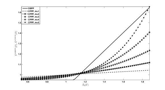
Figure 1: CPPP and OBPP payoffs as functions of $\hat{S}_{2}(T)$ according to (20) and (14) for the standard parameter set provided in Table 1 and $m=1,2,...,5$.

The graph visualizes the strategy payoffs according to (14) and (20) as functions of the terminal index ratio $\hat{S}_{2}(T)$, i.e. the standard OBPI and CPPI in the discounted market. With respect to the CPPP strategy different values of the multiplier $m=1,...,5$ are analyzed. For each value of the multiplier the payoffs intersect at least once. The CPPP payoff exceeds the OBPP one not only for very large values of the index ratio but also for the more important range of moderate outperformance and even underperformance of the active asset with respect to the reserve asset. For $m=1$ it is a linear and for $m>1$ an exponential function of $\hat{S}_{2}$. As the value of the multiplier increases, the CPPP portfolio value becomes more convex in $\hat{S}_{2}$. In contrast, the OBPP payoff is a (piecewise) linear function of the terminal index ratio.

The examination of the terminal performances is only a first step within the scope of a comparison of the two strategies. However, a detailed analysis must also take into account the entire payoff distributions - including the probabilities of bullish and bearish markets. In the sequel we will thus derive explicit formulas for the moments of the resulting distributions. This enables us to extend the analysis especially to the first four moments.

3.2 Comparison of the moments of the payoff distributions

3.2.1 Moments of the CPPP and the OBPP strategy

To derive explicit formulas for the moments of the payoff distributions of the OBPP and the CPPP we will make use of the similarity of performance participation and portfolio insurance strategies according to (14) and (20). As a byproduct we obtain general formulas for the moments of the standard OBPI and CPPI, too.

Lemma 6.

Let $V^{PP}(t)$ denote the portfolio value of the OBPP or the CPPP strategy at time $t\in[0,T]$ and $\hat{V}^{PI}(t)$ the respective value of the corresponding portfolio insurance strategy in the discounted market according to (14) and (20). Then, the $k$th moment $m_{k}\left(V^{PP}(t)\right)$, $k\in\mathbb{N}$ of the performance participation strategy PP with respect to the real-world measure $\mathbb{P}$ can be calculated as

$$m_{k}\left(V^{PP}(t)\right)=\mathbb{E}_{\mathbb{P}}\left[S_{1}(t)^{k}\right]\cdot\tilde{m}_{k}\left(\hat{V}^{PI}(t)\right),$$ (25)

where $\tilde{m}_{k}\left(\hat{V}^{PI}(t)\right)$ denotes the $k$th moment of the associated portfolio insurance strategy with respect to the equivalent probability measure $\tilde{\mathbb{P}}_{k}$ defined by the Radon-Nikodym derivative

$$\begin{array}[]{cc}\left.\frac{d\tilde{\mathbb{P}}_{k}}{d\mathbb{P}}\right|_{\mathcal{F}_{t}}=\tilde{Z}_{k}(t),&\tilde{Z}_{k}(t)=\frac{S_{1}(t)^{k}}{\mathbb{E}_{\mathbb{P}}\left[S_{1}(t)^{k}\right]}=exp\left\{k\cdot\sigma_{1}\cdot W_{1}(t)-\frac{1}{2}\cdot k^{2}\cdot\sigma_{1}^{2}\cdot t\right\},\end{array}$$ (26)

and

$$\mathbb{E}_{\mathbb{P}}\left[S_{1}(t)^{k}\right]=S_{1}(0)^{k}\cdot e^{k\cdot\mu_{1}\cdot t+\frac{1}{2}\cdot k\cdot(k-1)\cdot\sigma_{1}^{2}\cdot t}.$$ (27)

Proof.

The proof is given in A. ∎

Thus, similar to the portfolio values themselves the moments of the payoff distributions of the performance participation strategies are directly linked to the moments of the corresponding portfolio insurance strategies in the discounted market. However, an additional change of probability measure has to be conducted.

In the following, we generally derive the $k$th moments of the payoffs of a standard OBPI and CPPI strategy. Note that the calculation of the expected value as well as the variance was e.g. already proceeded in Bertrand and Prigent (2005) (expectation only) or Zagst and Kraus (2009). We start with the CPPI.

Proposition 7 (CPPI moments).

The $k$th moment, $k\in\mathbb{N}$, of a standard CPPI portfolio with level of insurance $\alpha^{PI}\leq e^{r\cdot T}$ and multiplier $m$ at any time $t\in[0,T]$ is given by

$$m_{k}\left(V^{CPPI}(t)\right)=\left(\alpha^{PI}\cdot V_{0}\right)^{k}\cdot\sum_{i=0}^{k}{k\choose i}\cdot e^{-k\cdot r\cdot(T-t)}\cdot\left(\frac{1-\alpha^{PI}\cdot e^{-r\cdot T}}{\alpha^{PI}\cdot e^{-r\cdot T}}\right)^{i}\cdot e^{i\cdot m\cdot\left[\mu_{S}-r+\frac{1}{2}\cdot(i-1)\cdot m\cdot\sigma_{S}^{2}\right]\cdot t}.$$ (28)

Proof.

The proof is given in B. ∎

A more sophisticated calculation leads to the following general analytic expression for the moments of the OBPI payoff distribution.

Theorem 8 (OBPI moments).

The $k$th moment, $k\in\mathbb{N}$, of the payoff of a standard OBPI strategy with level of portfolio insurance $\alpha^{PI}\leq e^{r\cdot T}$ at maturity $T$ is given by

$$m_{k}\left(V^{OBPI}(T)\right)$$ (29)

$$=\left(\alpha^{PI}\cdot V_{0}\right)^{k}+\left(\alpha^{PI}\cdot V_{0}\right)^{k}\cdot\sum_{i=1}^{k}\sum_{l=0}^{i}{k\choose i}\cdot{i\choose l}\cdot(-1)^{i-l}\cdot\left(\frac{p^{PI}\cdot S_{0}}{\alpha^{PI}\cdot V_{0}}\right)^{l}\cdot e^{l\cdot\mu_{S}\cdot T+\frac{1}{2}\cdot l\cdot(l-1)\cdot\sigma_{S}^{2}\cdot T}\cdot\Phi\left(d_{1,l}\right),$$

where

$$d_{1,l}=\frac{\ln\left(\frac{p^{PI}S_{0}}{\alpha^{PI}\cdot V_{0}}\right)+\left[\mu_{S}+\left(l-\frac{1}{2}\right)\cdot\sigma_{S}^{2}\right]\cdot T}{\sigma_{S}\cdot\sqrt{T}}.$$ (30)

Proof.

The proof is provided in C. ∎

According to Lemma 6 the $k$th moments of the performance participation strategies follow from the $k$th moments of the corresponding portfolio insurance strategies with respect to the equivalent probability measure $\tilde{\mathbb{P}}_{k}$ in the discounted market. The corresponding asset characteristics are provided in the following remark.

Remark 9.

The stochastic dynamics of the index ratio $\hat{S}_{2}=S_{2}/S_{1}$ with respect to the equivalent probability measure $\tilde{\mathbb{P}}_{k}$, $k\in\mathbb{N}$ defined in Equation (26) are given by

$$d\hat{S}_{2}(t)=\hat{S}_{2}(t)\hat{\mu}_{2,\tilde{k}}dt+\hat{S}_{2}(t)\hat{\sigma}_{2}d\tilde{W}_{\hat{S}_{2}}(t),\ \ \hat{S}_{2}(0)=1,$$ (31)

with drift

$$\hat{\mu}_{2,\tilde{k}}=\hat{\mu}_{2}+k\cdot\left(\rho_{12}\cdot\sigma_{1}\cdot\sigma_{2}-\sigma_{1}^{2}\right)=\left(\mu_{2}-\mu_{1}\right)+(k-1)\cdot\left(\rho_{12}\cdot\sigma_{1}\cdot\sigma_{2}-\sigma_{1}^{2}\right),$$ (32)

diffusion $\hat{\sigma}_{2}$ as defined in Equation (11) and Wiener process

$$\tilde{W}_{\hat{S}_{2},k}=\frac{\rho_{12}\cdot\sigma_{2}-\sigma_{1}}{\hat{\sigma}_{2}}\cdot\tilde{W}_{1,k}+\frac{\sqrt{1-\rho_{12}^{2}}\cdot\sigma_{2}}{\hat{\sigma}_{2}}\cdot\tilde{W}_{2,k}.$$ (33)

The risk-free interest rate $\hat{r}=0$ remains the same under the change of probability measure.

Proof.

The stochastic dynamics of $\hat{S}_{2}$ under the real-world measure $\mathbb{P}$ are given in Remark 2. Then, following from the Girsanov theorem the stochastic process $\bm{\tilde{W}_{k}}(t)=\left(\tilde{W}_{1,k}(t),\tilde{W}_{2,k}(t)\right)^{\prime}$, $0\leq t\leq T$ defined by

$$\tilde{W}_{1,k}(t) :=W_{1}(t)-k\cdot\sigma_{1}\cdot t,$$ (34)

$$\tilde{W}_{2,k}(t) :=W_{2}(t),$$ (35)

is a two-dimensional Brownian motion under the equivalent probability measure $\tilde{\mathbb{P}}_{k}$, $k\in\mathbb{N}$. Substituting (34) and (35) in (16) proves the proposition. ∎

The moments of the CPPP and the OBPP strategy are then finally derived.

Lemma 10 (CPPP moments).

The $k$th moment, $k\in\mathbb{N}$, of a CPPP portfolio with level of performance participation $\alpha<1$ and multiplier $m$ at any time $t\in[0,T]$ is given by

$$m_{k}\left(V^{CPPP}\left(t;T,V_{0},\alpha,m,S_{1},S_{2}\right)\right)=\alpha^{k}\cdot\mathbb{E}_{\mathbb{P}}\left[S_{1}(t)^{k}\right]\cdot\sum_{i=0}^{k}{k\choose i}\cdot\left(\frac{1-\alpha}{\alpha}\right)^{i}\cdot e^{i\cdot m\cdot\left[\hat{\mu}_{2,\tilde{k}}+\frac{1}{2}\cdot(i-1)\cdot m\cdot\hat{\sigma}_{2}^{2}\right]\cdot t},$$ (36)

where $\mathbb{E}_{\mathbb{P}}\left[S_{1}(t)^{k}\right]$, $\hat{\mu}_{2,\tilde{k}}$ and $\hat{\sigma}_{2}^{2}$ as defined above.

Proof.

Substituting $\hat{V}_{0}=1$, $\hat{r}=0$, (32), (11) and (28) in (25) leads to the proposition.∎

Lemma 11 (OBPP moments).

The $k$th moment, $k\in\mathbb{N}$, of the payoff of an OBPP strategy with level of performance participation $\alpha<1$ at maturity $T$ is given by

$$m_{k}\left(V^{OBPP}\left(T;T,V_{0},\alpha,S_{1},S_{2}\right)\right)$$ (37)

$$=\alpha^{k}\cdot\mathbb{E}_{\mathbb{P}}\left[S_{1}(t)^{k}\right]\cdot\left\{1+\sum_{i=1}^{k}\sum_{l=0}^{i}{k\choose i}\cdot{i\choose l}\cdot(-1)^{i-l}\cdot\left(\frac{p}{\alpha}\right)^{l}\cdot e^{l\cdot\left[\hat{\mu}_{2,\tilde{k}}+\frac{1}{2}\cdot(l-1)\cdot\hat{\sigma}_{2}^{2}\right]\cdot T}\cdot\Phi\left(\hat{d}_{k,l}\right)\right\},$$

where

$$\hat{d}_{k,l}=\frac{\ln\left(\frac{p}{\alpha}\right)+\left[\hat{\mu}_{2,\tilde{k}}+\left(l-\frac{1}{2}\right)\cdot\hat{\sigma}_{2}^{2}\right]\cdot T}{\hat{\sigma}_{2}\cdot\sqrt{T}}.$$ (38)

Proof.

Substituting $\hat{V}_{0}=1$, (32), (11), strike $\alpha$ and (29) in (25) leads to the proposition. ∎

With the above general expressions for the $k$th moments we have all the essential information to describe the entire payoff distributions of the two performance participation (portfolio insurance) strategies. The usually reported central moments are obtained by a final transformation.

Remark 12 (Central moments).

By applying the binomial theorem the $k$th central moment $\mu_{k}(V)$ of a random variable $V$ follows directly from its $i$th moment $m_{i}(V)$, $i=0,...,k$ by

$$\mu_{k}(V)=\mathbb{E}_{\mathbb{P}}\left[\left(V-\mathbb{E}_{\mathbb{P}}[V]\right)^{k}\right]=\sum_{i=0}^{k}{k\choose i}\cdot(-1)^{k-i}\cdot m_{i}(V)\cdot\left(m_{1}(V)^{k-i}\right).$$ (39)

In the sequel we will especially compare the first four (central) moments of the payoff distributions of the two performance participation strategies in more detail. We start with the expected strategy payoffs. As mentioned earlier, with respect to the CPPP strategy we will analyze various values of the multiplier $m$, among them the unique value $m^{*}$ for which the expectations of the two strategies are equal. Its derivation and analysis is the focus of the following section.

3.2.2 Equality of payoff expectations

The expected payoffs of the CPPP and the OBPP follow directly from Lemma 10 and Lemma 11 as the first moments of the resulting terminal portfolio value distributions

$$\mu\left(V^{CPPP}\left(T;T,V_{0},\alpha,m,S_{1},S_{2}\right)\right) =m_{1}\left(V^{CPPP}\left(T;T,V_{0},\alpha,m,S_{1},S_{2}\right)\right)$$ (40)

$$=\alpha\cdot V_{0}\cdot e^{\mu_{1}\cdot T}+\left(1-\alpha\right)\cdot V_{0}\cdot e^{\left[\mu_{1}+m\cdot\left(\mu_{2}-\mu_{1}\right)\right]\cdot T},$$

$$\mu\left(V^{OBPP}\left(T;T,V_{0},\alpha,S_{1},S_{2}\right)\right) =m_{1}\left(V^{OBPP}\left(T;T,V_{0},\alpha,S_{1},S_{2}\right)\right)$$ (41)

$$=\alpha\cdot V_{0}\cdot e^{\mu_{1}\cdot T}+V_{0}\cdot e^{\mu_{2}\cdot T}\cdot Call\left(0;T,\alpha,\hat{\mu}_{2,\tilde{1}},\hat{\sigma}_{2},p\cdot\hat{S}_{2}\right)$$

$$=\alpha\cdot V_{0}\cdot e^{\mu_{1}\cdot T}\cdot\left(1-\Phi\left(\hat{d}_{1,0}\right)\right)+p\cdot V_{0}\cdot e^{\mu_{2}\cdot T}\cdot\Phi\left(\hat{d}_{1,1}\right),$$

where $\hat{\mu}_{2,\tilde{1}}=\mu_{2}-\mu_{1}$ and $\hat{d}_{k,l}$, $l=0,1$ as defined in (38).

The expected payoff of the CPPP strategy is independent of the variance-covariance structure of the underlying risky assets. Thus, the expected return is not affected by the additional source of risk. Moreover, it is an exponentially growing function in the value of the multiplier $m$ if and only if the further condition $\mu_{1}<\mu_{2}$ is satisfied. Since the multiplier controls the exposure to the active asset $S_{2}$ this is a natural expectation from the CPPP payoff sensitivity and justifies our initial assumption made in Section 2.1. In contrast, an increase in the desired level of performance participation $\alpha$ (exponentially) reduces the expected payoff (in case that $\mu_{1}<\mu_{2}$). The enhanced participation guarantee in the reserve asset comes at the price of a diminished cushion and thus less upside potential stemming from a potential outperformance of the active asset $S_{2}$.

With respect to the expected payoff of the OBPP strategy we observe an analog sensitivity on the fraction $\alpha$. As motivated in Section 2.2 an increase in $\alpha$ is accompanied by a decrease in the number of shares/exchange options $p$.

Equating the two expectations (40) and (41) leads to the following proposition.

Lemma 13 (Multiplier $m^{*}$).

For any parameterization of the financial market (1) and any level of performance participation $\alpha<1$ there exists a unique value $m^{*}\left(\alpha,\mu_{2}-\mu_{1},\hat{\sigma}_{2},T\right)$ of the multiplier such that

$$\mu\left(V^{CPPP}\left(T;T,V_{0},\alpha,m^{*},S_{1},S_{2}\right)\right)=\mu\left(V^{OBPP}\left(T;T,V_{0},\alpha,S_{1},S_{2}\right)\right),$$

which is given by

$$m^{*}\left(\alpha,\mu_{2}-\mu_{1},\hat{\sigma}_{2},T\right)=1+\frac{1}{\left(\mu_{2}-\mu_{1}\right)\cdot T}\cdot\ln\left(\frac{Call\left(0;T,\alpha,\mu_{2}-\mu_{1},\hat{\sigma}_{2},p\cdot\hat{S}_{2}\right)}{Call\left(0;T,\alpha,\hat{r},\hat{\sigma}_{2},p\cdot\hat{S}_{2}\right)}\right).$$ (42)

Here, $Call\left(t;T,\alpha,r_{f},\hat{\sigma}_{2},p\cdot\hat{S}_{2}\right)$ denotes the Black-Scholes value of a vanilla call option written on $p$ shares of asset $\hat{S}_{2}$ with strike $\alpha$, risk-free interest rate $r_{f}$, volatility $\hat{\sigma}_{2}$, evaluated at time $t$ for maturity $T$.

Proof.

Following from (14) and (20) the problem can be reduced to the equivalent problem for the standard portfolio insurance strategies in the discounted world and with respect to the equivalent probability measure $\tilde{\mathbb{P}}_{1}$ , i.e.

$$\mathbb{E}_{\tilde{\mathbb{P}}_{1}}\left[\hat{V}^{CPPI}\left(T;T,\hat{V}_{0},\alpha,m^{*},\hat{r},\hat{S}_{2}\right)\right]=\mathbb{E}_{\tilde{\mathbb{P}}_{1}}\left[\hat{V}^{OBPI}\left(T;T,\hat{V}_{0},\alpha,\hat{r},\hat{S}_{2}\right)\right],$$

where $\hat{V}_{0}=1$ and $\hat{r}=0$. The stochastic dynamics of $\hat{S}_{2}$ with respect to $\tilde{\mathbb{P}}_{1}$ are provided in (31). This issue was already solved in Bertrand and Prigent (2005) yielding the proposed multiplier $m^{*}$. ∎

Note that since $\mu_{2}>\mu_{1}$ and thus $Call\left(0;T,\alpha,\mu_{2}-\mu_{1},\hat{\sigma}_{2},p\cdot\hat{S}_{2}\right)>Call\left(0;T,\alpha,\hat{r},\hat{\sigma}_{2},p\cdot\hat{S}_{2}\right)$ the value of the multiplier $m^{*}$ is always bigger than one. For any value of the multiplier $m>m^{*}$ the expected payoff of the CPPP strategy exceeds that of the OBPP strategy and vice versa.

The special multiplier $m^{*}$ is an increasing function of the investor-defined level of performance participation $\alpha<1$. This sensitivity was already motivated in Bertrand and Prigent (2005) for the standard OBPI and CPPI. Although both expected payoffs are decreasing in the fraction $\alpha$ the CPPP is usually more sensitive to its variation. This is mainly caused by the leveraging effect of the multiplier that exponentially amplifies the reduction of the cushion.

As an example, Figure 2 visualizes the evolution of $m^{*}$ as a function of the level of performance participation $\alpha$ for the standard case presented in Table 1. With respect to the standard level of performance participation $\alpha=0.95$ the multiplier $m^{*}$ according to Equation (42) yields $m^{*}\left(0.95,3.1\%,22.3\%,1\right)=6.90$. Note that since the risky reserve asset features a higher drift than the risk-free asset the associated lower excess return will usually induce higher values of the multiplier $m^{*}$ than it is the case for the standard CPPI strategy.

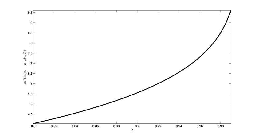
Figure 2: Multiplier $m^{*}$ as a function of the investor-defined level of performance participation $\alpha$ for the standard parameter setup provided in Table 1.

Furthermore, $m^{*}$ is a decreasing function in the excess drift $\mu_{2}-\mu_{1}$. Although both expected values are increasing in the drift difference, again the CPPP payoff reacts usually more sensitively to a change as it is amplified by the multiplier $m$. Thus, for higher excess drifts a smaller value of $m$ is sufficient to maintain an equivalent level of return expectation.

In the next step we include higher (central) moments in our analysis. Since the payoffs under consideration are non-linear a mean-variance approach is not sufficient. This leads us to examine, besides expectation, also standard deviation, skewness and kurtosis.

3.2.3 Comparison of the first four moments

Table 2 provides the obtained values for the expectation ($\mu$), standard deviation ($\sigma$), skewness ($\gamma_{3}$) and kurtosis ($\gamma_{4}$) of the returns of the OBPP and the CPPP strategy in the case of the standard parameterization provided in Table 1. With respect to the CPPP strategy different values of the multiplier $m$ are analyzed including the special value $m^{*}$. Note that for the sake of simplicity the results are given in a return dimension instead of the usual portfolio value dimension.

	OBPP	CPPP
	$\alpha=0.95$	$m^{*}=6.90$	$m=3$	$m=5$	$m=6$	$m=7$	$m=8$
$\mu$	8.10%		7.34%	7.72%	7.91%	8.12%	8.33%
$\sigma$	12.37%	19.92%	5.02%	9.58%	13.92%	20.74%	31.84%
$\gamma_{3}$	2.3606	37.7639	1.1672	7.6060	16.9331	41.4930	118.2519
$\gamma_{4}$	7.4806	1.3912$\cdot 10^{4}$	5.3743	222.9118	1.6409$\cdot 10^{3}$	1.7946$\cdot 10^{4}$	3.0765$\cdot 10^{5}$

Table 2: Expectation, standard deviation, skewness and kurtosis of the payoff distributions of an OBPP strategy and CPPP strategies with different multipliers for the standard parameterization provided in Table 1.

We obtain comparable results as for standard portfolio insurance strategies (see Bertrand and Prigent (2005)). Both strategies generate an asymmetric payoff profile. However, due to the significantly higher positive skewness of the CPPP in comparison to the OBPP, it should be preferred with respect to that criterion. Furthermore, the strategy’s (excess) kurtosis largely exceeds that of the OBPP. This feature is explained by the outperformance of the dynamic strategy in the right tail of the distribution where $\hat{S}_{2}(T)>>1$.

When differing from the special multiplier $m=m^{*}$ to consider more general values of $m$, we have to distinguish two situations. If the multiplier $m$ is higher than $m^{*}$, then the CPPP strategy provides a higher expected payoff than the OBPP. The improved upside potential/intensified participation in the better returning asset $S_{2}$ is not for free and comes at the price of more risk, i.e. an increasing standard deviation. Since the CPPP thus exceeds the risk associated with the OBPP, none of the two strategies dominates the other one in a mean-variance sense.

In contrast, if the multiplier $m$ takes smaller values than $m^{*}$, then both the expected CPPP payoff as well as the strategy’s standard deviation are decreasing. Thus, the CPPP provides a smaller return expectation than the OBPP. Furthermore, for small negative deviations of $m$ with respect to $m^{*}$ the risk of the OBPP will still remain less than that associated with the CPPP. Consequently the OBPP strictly dominates the CPPP in a mean-variance sense. Nevertheless, for sufficiently large differences $m^{*}-m$ both the expected payoff as well as the standard deviation of the CPPP strategy take smaller values than the OBPP ones. Hence, none of the strategies dominates the other one with respect to the mean-variance criterion.

Bertrand and Prigent (2005) further analyze the probability distributions associated with the standard OBPI and the standard CPPI strategy with a special focus on the payoff ratio $\frac{V^{OBPI}(T)}{V^{CPPI}(T)}$. Among others they conclude that for usual values of the multiplier the probability that the CPPI outperforms the OBPI at the terminal date is increasing in the level of insurance. As the probability of exercising the call option at maturity decreases with the increasing strike, the upside potential of the OBPI strategy is significantly reduced. Due to the special relationship between performance participation and portfolio insurance strategies following from (14) and (20) this result remains valid for the more general OBPP and CPPP, as

$$\frac{V^{OBPP}(T)}{V^{CPPP}(T)}=\frac{\hat{V}^{OBPI}(T)}{\hat{V}^{CPPI}(T)}.$$

For further details of the analysis we refer the interested reader to Bertrand and Prigent (2005).

In the following we will briefly study the dynamic properties of the two strategies and in particular their "Greeks". Due to the elaborated relationship between performance participation and standard portfolio insurance strategies the analysis can be kept short for sensitivities where the additional source of risk is not of direct interest.

4 The Dynamic Behavior of OBPP and CPPP

With respect to the practical realization of the OBPP strategy, in many situations the use of standardized traded options is not possible. For example, the underlying(s) may be a diversified fund for which no single option is available. Furthermore, the desired investment period may also not coincide with the maturity of a listed option. OTC options, on the other hand, involve several drawbacks like counterparty risk or liquidity problems and raise the question for the fair price of the contingent claim.

In practice, the underlying exchange options are thus usually synthesized by dynamic replication. In the presumed Black-Scholes model (1) the perfect hedging strategy according to the Margrabe formula (8) exists. Based on the induced dynamic hedging rule one can show that the OBPP strategy actually represents a generalized CPPP strategy with time-variable multiplier. Moreover, the study of the derived multiplier allows to quantify the risk exposure associated with the OBPP strategy.

Since in practice the number of rebalancing trades is limited due to the associated transaction costs, the dynamic replication of the exchange option induces hedging risks. This is the reason why we also analyze the hedging properties (i.e. the Greeks) of both methods. Special focus is put on the behavior of the exposures to the two risky underlyings during the investment period.

4.1 OBPP as generalized CPPP

For the CPPP method the multiplier $m$ is the key parameter that controls the amount invested in the active asset $S_{2}$ and the possible leverage associated with it. Moreover, as shown in Section 3.2.1, it directly affects the risk-return ratio of the resulting portfolio. Knowing about the importance of the multiplier, Bertrand and Prigent (2005) were able to show for the standard OBPI strategy the existence of such an "implicit"’ parameter. This finding remains valid for the two-asset OBPP strategy. The respective implicit multiplier for the OBPP is deduced in the following proposition.

Lemma 14 (OBPP multiplier).

The OBPP method is equivalent to a generalized CPPP method with time-variable multiplier given by

$$m^{OBPP}\left(t;\alpha,S_{1},S_{2}\right)=\frac{p\cdot S_{2}(t)\cdot\Phi\left(d_{1}\right)}{V^{ex}\left(t;T,p\cdot S_{2},\alpha\cdot S_{1}\right)}=\frac{p\cdot\hat{S}_{2}(t)\cdot\Phi\left(d_{1}\right)}{Call\left(t;T,\alpha,\hat{r},\hat{\sigma}_{2},p\cdot\hat{S}_{2}\right)},$$ (43)

where $d_{1}$ as defined in (9).

Proof.

The proposition follows directly from Bertrand and Prigent (2005)’s result for standard CPPI strategies and the similarity of performance participation and portfolio insurance according to (14) and (20) as well as (15). ∎

In analogy to the CPPP strategy the OBPP multiplier is equal to the ratio of the exposure to the active asset $S_{2}$ and the OBPP cushion. The former is given by the amount invested in asset $S_{2}$ to replicate the exchange option $V^{ex}\left(t;T,p\cdot S_{2},\alpha\cdot S_{1}\right)$ and the latter by the value of the exchange option itself. In terms of the discounted asset universe, respectively, this is equal to the exposure to $\hat{S}_{2}$ to replicate the corresponding call option on the relative asset $\hat{S}_{2}$ divided by the OBPI cushion, which is the call value.

As an example Figure 3 visualizes the OBPP multiplier as a function of the index ratio $\hat{S}_{2}$ at time $t=0.25,0.5,0.75$ for the case of the standard parameterization provided in Table 1.

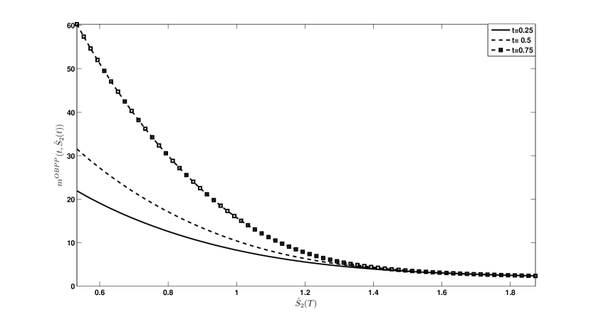
Figure 3: OBPP multiplier $m^{OBPP}\left(t;\alpha,\hat{S}_{2}\right)$ as a function of the index ratio $\hat{S}_{2}$ at time $t=0.25,0.5,0.75$ for the standard parameterization provided in Table 1.

Hence, the OBPP multplier is at any time $t\in[0,T]$ a decreasing function of the index ratio $\hat{S}_{2}$. Furthermore, following from the Margrabe formula (8) it is always bigger than $1$.

It can be easily seen that the OBPP multiplier usually takes higher values than that of standard CPPP strategies, except for the case when the active asset $S_{2}$ significantly outperforms the reserve asset $S_{1}$ and the associated exchange or call option, respectively, is thus (deeply) in the money. This is due to the small values of the OBPP cushion, i.e. the value of the exchange option, when the index ratio $\hat{S}_{2}$ is small.

The high values of the multiplier involve potential risk when the market drops suddenly: it means that either the OBPP cushion is too small or the exposure to the riskier asset is too high. In contrast, with an increasing outperformance of the active asset $S_{2}$ over the reserve asset $S_{1}$ the low values of the multiplier prevent the OBPP portfolio from being overinvested in the riskier asset. Nevertheless, a direct implication of that feature is that in the case of a sustainable outperformance of the active asset over the entire investment period, without any drop, the CPPP strategy will perform better due to the higher active exposure.

To conclude the analysis of $m^{OBPP}$ Figure 4 visualizes the evolution of the cumulative distribution function of the OBPP multiplier over time for the standard parameter set provided in Table 1.

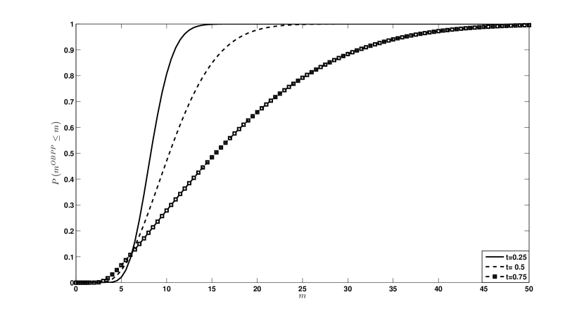
Figure 4: Evolution of the cumulative distribution function of $m^{OBPP}$ for $t=0.25,0.5,0.75$ and the standard parameter set provided in Table 1.

As time increases, the probability of obtaining higher values of the OBPP multiplier increases. Bertrand and Prigent (2005) argue that this is essentially due to the rise of variance with time.

In the next step we will analyze the Greeks of the OBPP and the CPPP in more detail which represent the dynamic hedging properties of the two performance participation strategies.

4.2 The Greeks of the performance participation strategies

We start with the delta representing one of the main concerns of a portfolio manager.

4.2.1 The delta

Recall that the delta $\Delta$ measures the rate of change of the portfolio value with respect to changes in the underlying asset prices. In the case of the OBPP the sensitivities of the strategy performance on the asset performances follow directly from the deltas of the underlying exchange option. An analog calculation as for the derivation of the delta of a vanilla call option yields

$$\Delta_{1}^{OBPP}(t) =\frac{\partial V^{OBPP}(t)}{\partial S_{1}(t)}=\alpha\cdot\Phi\left(-d_{2}\right)=\alpha\cdot\left(1-\Phi\left(d_{2}\right)\right),$$

$$\Delta_{2}^{OBPP}(t) =\frac{\partial V^{OBPP}(t)}{\partial S_{2}(t)}=p\cdot\Phi\left(d_{1}\right).$$

The deltas of the OBPP strategy are always positive, smaller (or equal) to one and tend to $0$ ($1$) and $1$ ($0$) as the investment horizon approaches its end and $p\cdot\hat{S}_{2}>\alpha$ ($p\cdot\hat{S}_{2}<\alpha$), respectively. In contrast, if the option is at-the-money, i.e. $p\cdot\hat{S}_{2}=\alpha$, the deltas converge to $\frac{\alpha}{2}$ and $\frac{p}{2}$, respectively, as time to maturity approaches zero. This limiting behavior is easy to understand from the payoff structure of the exchange option: as the time to maturity tends to zero the OBPP portfolio is mainly invested in the better performing asset. However, no leveraging is included.

For the CPPP strategy the deltas follow by partial differentiation of the portfolio value (21) as

$$\Delta_{1}^{CPPP}(t) =\frac{\partial V^{CPPP}(t)}{\partial S_{1}(t)}=\alpha+(1-m)\cdot\beta_{CPPP}\left(t;\alpha,m,\hat{\sigma}_{2}\right)\cdot\left(\frac{S_{2}(t)}{S_{1}(t)}\right)^{m},$$ (44)

$$\Delta_{2}^{CPPP}(t) =\frac{\partial V^{CPPP}(t)}{\partial S_{2}(t)}=m\cdot\beta_{CPPP}\left(t;\alpha,m,\hat{\sigma}_{2}\right)\cdot\left(\frac{S_{2}(t)}{S_{1}(t)}\right)^{m-1}.$$ (45)

Whereas similar to the OBPP strategy $\Delta_{2}^{CPPP}$ is always positive, $\Delta_{1}^{CPPP}$ is always smaller than the level of performance participation $\alpha<1$ and especially for high values of the multiplier $m>1$ and a strong outperformance of $S_{2}$ with respect to $S_{1}$ likely to take (highly) negative values. Simultaneously, the $\Delta_{2}^{CPPP}$ is then very likely to take significantly higher values than one. The observed sensitivity is due to the convex leveraging feature of the CPPP strategy in the active asset. The strategy value as well as $\Delta_{2}^{CPPP}$ become the more convex in $S_{2}$ the higher the value of the multiplier $m$. A high stochastic floor in terms of $S_{1}$ thus significantly reduces the cushion and the overall performance of the strategy. Furthermore, since $\beta_{CPPP}\left(t;\alpha,m,\hat{\sigma}_{2}\right)$ is a decreasing function in time $t$, $\Delta_{1}^{CPPP}$ is increasing and $\Delta_{2}^{CPPP}$ is decreasing with time.

Figure 5 and 6 show the evolution of the deltas of the two performance participation strategies with respect to the reserve asset $S_{1}$ and the active asset $S_{2}$ as functions of the index ratio $\hat{S}_{2}$ at time $t=0.75$. The standard parameter set given in Table 1 is applied. With respect to the CPPP strategy different values of the multiplier are analyzed.

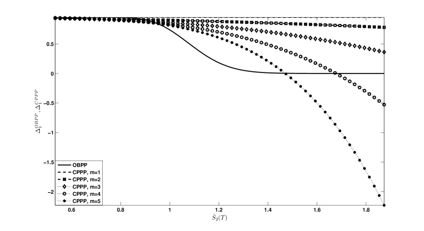
Figure 5: OBPP and CPPP delta with respect to the reserve asset $S_{1}$ as a function of the index ratio $\hat{S}_{2}$ at time $t=0.75$. The standard parameter set provided in Table 1 is applied. With respect to the CPPP the multipliers $m=1,2,3,4,5$ are analyzed.

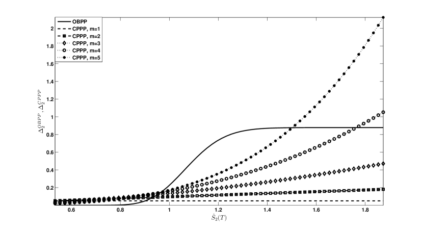
Figure 6: OBPP and CPPP delta with respect to the active asset $S_{2}$ as a function of the index ratio $\hat{S}_{2}$ at time $t=0.75$. The standard parameter set provided in Table 1 is applied. With respect to the CPPP the multipliers $m=1,2,3,4,5$ are analyzed.

Notice that for moderate $\hat{S}_{2}>1$, i.e. when the exchange (or the discounted call) option is in-the-money, the OBPP delta with respect to the active asset $S_{2}$ (with respect to the reserve asset $S_{1}$) is greater (smaller) than that of the CPPP one. This induces a higher risk of the option-based strategy in the case of a sudden market downturn of $S_{2}$ relative to $S_{1}$. In contrast, if the active asset significantly outperforms the reserve asset, i.e. when the option is deeply in-the-money, then the CPPP fall exceeds the OBPP one.

Bertrand and Prigent (2005) analyze the delta of standard portfolio insurance strategies in more detail. In fact, due to the relationship between performance participation and portfolio insurance strategies according to (14) and (20) the deltas of the the OBPP and the CPPP with respect to the active asset $S_{2}$ are actually equal to the deltas of the corresponding standard portfolio insurance strategies with respect to the discounted underlying $\hat{S}_{2}$

$$\Delta_{2}^{PP}(t)=\frac{\partial V^{PP}(t)}{\partial S_{2}(t)}=\frac{\partial S_{1}(t)\cdot\hat{V}^{PI}(t)}{\partial S_{2}(t)}=\frac{\partial\hat{V}^{PI}(t)}{\partial\hat{S}_{2}(t)}=\hat{\Delta}^{PI}.$$

Thus, all results derived by Bertrand and Prigent (2005) remain valid for the generalized performance participation strategies in terms of the index ratio $\hat{S}_{2}$ instead of the former risky asset $S$. Among others they show that in probability the CPPP is significantly less sensitive to the ratio $\hat{S}_{2}$ than the OBPP.

Next we will analyze the gamma of the OBPP and the CPPP that measures the convexity of the portfolio values in the underlying asset prices. It is important to ensure an effective delta hedge.

4.2.2 The gamma

Recall that the gamma $\Gamma$ measures the rate of change in the delta with respect to changes in the underlying prices. In the case of the OBPP it follows directly from the gamma of the underlying exchange option. An analog calculation to the derivation of a call option’s gamma yields

$$\Gamma_{1}^{OBPP}(t) =\frac{\partial^{2}V^{OBPP}(t)}{\partial S_{1}(t)^{2}}=\alpha\cdot\frac{\varphi\left(-d_{2}\right)}{S_{1}(t)\cdot\hat{\sigma}_{2}\cdot\sqrt{T-t}}=\alpha\cdot\frac{\varphi\left(d_{2}\right)}{S_{1}(t)\cdot\hat{\sigma}_{2}\cdot\sqrt{T-t}},$$

$$\Gamma_{2}^{OBPP}(t) =\frac{\partial^{2}V^{OBPP}(t)}{\partial S_{2}(t)^{2}}=p\cdot\frac{\varphi\left(d_{1}\right)}{S_{2}(t)\cdot\hat{\sigma}_{2}\cdot\sqrt{T-t}}.$$

Hence, the OBPP gammas are always positive and converge - except for the at-the-money-case - to zero as the option approaches its maturity. When the option is at-the-money, i.e. $p\cdot\hat{S}_{2}=\alpha$, then $d_{i}$, $i=1,2$ converges to zero and $\varphi\left(d_{i}\right)$ takes the value $\frac{1}{\sqrt{2\pi}}$. Overall, the gammas diverge to infinity in this case.

Analogously, the gammas of the CPPP strategy follow by partial differentiation of the derived deltas (44) and (45) as

$$\Gamma_{1}^{CPPP}(t) =\frac{\partial^{2}V^{CPPP}(t)}{\partial S_{1}(t)^{2}}=m\cdot(m-1)\cdot\beta_{CPPP}\left(t;\alpha,m,\hat{\sigma}_{2}\right)\cdot S_{1}(t)^{-1}\cdot\left(\frac{S_{2}(t)}{S_{1}(t)}\right)^{m},$$

$$\Gamma_{2}^{CPPP}(t) =\frac{\partial^{2}V^{CPPP}(t)}{\partial S_{2}(t)^{2}}=m\cdot(m-1)\cdot\beta_{CPPP}\left(t;\alpha,m,\hat{\sigma}_{2}\right)\cdot S_{2}(t)^{-1}\cdot\left(\frac{S_{2}(t)}{S_{1}(t)}\right)^{m-1}.$$

Thus, the CPPP gammas are always positive justifying the convex leveraging feature of the strategy.

Figure 7 and 8 visualize the OBPP and the CPPP gammas as a function of the index ratio $\hat{S}_{2}$ at time $t=0.75$. The standard parameterization provided in Table 1 is applied. With respect to the CPPP different values of the multiplier are analyzed. Note that the common factor $S_{1}(t)^{-1}$ or $S_{2}(t)^{-1}$ with respect to $\Gamma_{1}^{OBPP,CPPP}$ or $\Gamma_{2}^{OBPP,CPPP}$, respectively, has been omitted.

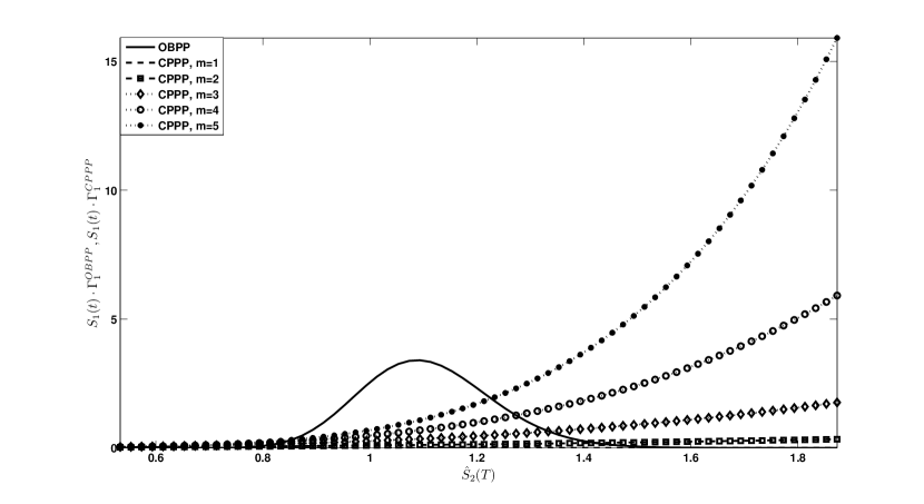
Figure 7: OBPP and CPPP gamma with respect to the reserve asset $S_{1}$ as a function of the index ratio $\hat{S}_{2}$ for $t=0.75$. The standard parameterization provided in Table 1 is applied. With respect to the CPPP the multipliers $m=1,2,3,4,5$ are analyzed.

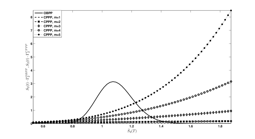
Figure 8: OBPP and CPPP gamma with respect to the active asset $S_{2}$ as a function of the index ratio $\hat{S}_{2}$ for $t=0.75$. The standard parameterization provided in Table 1 is applied. With respect to the CPPP the multipliers $m=1,2,3,4,5$ are analyzed.

With respect to the CPPP strategy the gammas are especially important for very high values of the index ratio $\hat{S}_{2}$. Nevertheless, for the most probable realizations of $\hat{S}_{2}$ around one, and especially when the exchange option is in-the-money, the CPPP gamma is smaller than the OBPP one for a large range of values. Furthermore, since $\beta_{CPPP}\left(t;\alpha,m,\hat{\sigma}_{2}\right)$ is monotonically decreasing in time $t$, the CPPP gammas are decreasing when approaching the end of the investment horizon; yet, they never reach zero. In contrast, with the time to maturity approaching zero the OBPP gammas will converge to zero for an in- or out-of-the money call and diverge if $p\cdot\hat{S}_{2}=\alpha$.

To conclude the section we briefly look at the portfolio vegas of the two performance participation strategies under consideration.

4.2.3 The vega

The vega measures the strategy’s sensitivity on the volatility(ies) of the underlying assets. Since both the CPPP and the OBPP portfolio value only depend on the aggregated volatility $\hat{\sigma}_{2}$ of the index ratio $\hat{S}_{2}$ we restrict our analysis of the vega to this special diffusion. We recall that $\hat{\sigma}_{2}$ is a decreasing function in the asset correlation $\rho_{12}$. Furthermore, using the assumption $\sigma_{1}<\sigma_{2}$ it is increasing in $\sigma_{2}$; with respect to $\sigma_{1}$ the sensitivity is ambigous.

Due to the special relationship between performance participation and portfolio insurance strategies according to (14) and (20) the vegas of the two strategies follow directly from the vegas of the underlying portfolio insurance strategies in the discounted market. More precisely, we obtain

$$\nu^{OBPP}(t) =\frac{\partial V^{OBPP}(t)}{\partial\hat{\sigma}_{2}}=p\cdot S_{1}(t)\cdot\hat{S}_{2}(t)\cdot\varphi\left(d_{1}\right)\cdot\sqrt{T-t}=p\cdot S_{2}(t)\cdot\varphi\left(d_{1}\right)\cdot\sqrt{T-t},$$

$$\nu^{CPPP}(t) =\frac{\partial V^{CPPP}(t)}{\partial\hat{\sigma}_{2}}=S_{1}(t)\cdot m\cdot(1-m)\cdot\hat{\sigma}_{2}\cdot t\cdot\left(\hat{V}^{CPPI}(t)-\hat{F}^{CPPI}(t)\right)$$

$$=-m\cdot(m-1)\cdot\hat{\sigma}_{2}\cdot t\cdot C(t).$$

Whereas the vega of the OBPP strategy is always positive, the vega of the CPPP strategy takes negative values for $m>1$. Thus, an increase in the volatility of the index ratio $\hat{S}_{2}$ reduces the actual CPPP portfolio value. The extent of the decrease is the larger the higher the value of the multiplier $m$ and the longer the elapsed investment time $t$ since inception. If $m=1$ the value of the CPPP strategy is independent on a change in the tracking error $\hat{\sigma}_{2}$. In contrast, the vega of the exchange/call option is positive, since an increase in the volatility increases the probability that the option will be executed at its expiry and thus its price. The closer the investment horizon approaches maturity the smaller is the impact of a change in $\hat{\sigma}_{2}$ since $\lim_{t\rightarrow T}\nu^{OBPP}(t)=0$.

As an example Figure 9 visualizes the discounted OBPP and CPPP vega as a function of the index ratio $\hat{S}_{2}$ at time $t=0.75$. The standard model parameterization provided in Table 1 is applied. With respect to the CPPP different values of the multiplier are analyzed.

Figure 9: Discounted OBPP and CPPP vega as functions of the index ratio $\hat{S}_{2}$ for $t=0.75$. The standard parameter set provided in Table 1 is applied. With respect to the CPPP different values of the multiplier are analyzed.

Table 3 summarizes the described sensitivities of the strategy Greeks with respect to the magnitude of the index ratio $\hat{S}_{2}$.

	$\hat{S}_{2}<<1$			$\hat{S}_{2}\approx 1$			$\hat{S}_{2}>>1$
	OBPP		CPPP	OBPP		CPPP	OBPP		CPPP
$\Delta_{1}$		$\approx$		neg.	$<$	neg.	neg.	$>>$	neg.
$\Delta_{2}$		$\approx$		pos.	$>$	pos.	pos.	$<<$	pos.
$\Gamma_{1}$		$\approx$		pos.	$>$	pos.	pos.	$<<$	pos.
$\Gamma_{2}$		$\approx$		pos.	$>$	pos.	pos.	$<<$	pos.
$\nu$		$\approx$		pos.	$>$	neg.	pos.	$>>$	neg.

Table 3: Sensitivities of the OBPP and CPPP Greeks with respect to the index ratio $\hat{S}_{2}$.

Overall, the two portfolios react in a similar way on a change in the value of the index ratio $\hat{S}_{2}$ or the associated volatility $\hat{\sigma}_{2}$ when the active asset is significantly outperformed by the reserve asset. Thus, neither of the two strategies can be preferred. In contrast, for exceptionally high values of $\hat{S}_{2}$ the CPPP strategy requires significantly more hedging effort than the OBPP as it is extremely sensitive on changes in the value of the active asset or the volatility of the index ratio. This sensitivity is even amplified with higher values of the multiplier $m$. Nevertheless, for the most probable realizations of the asset ratio $\hat{S}_{2}$ around one, the OBPP appears riskier with respect to a sudden market drop.

To conclude our analysis of the OBPP and the CPPP strategy we summarize the main results and give some concluding remarks.

5 Conclusion

In this paper we have introduced the class of performance participation strategies that guarantee a minimum return in terms of a percentage of a stochastic benchmark while keeping the potential for profits from the outperformance of a second, riskier asset. The new strategy class thus represents a generalization of the well-established portfolio insurance methods where the provided guarantee is not deterministic anymore but subject to systematic risk instead.

Moreover, with the OBPP and the CPPP we have presented a static as well as a dynamic example of a performance participation method that are closely related to the well-known OBPI and CPPI strategy. In fact, we have shown that the two strategy classes can be transformed into each other by discounting with the reserve asset as numéraire. Based on that very important relationship we were able to derive general analytic expressions not only for all of the moments of the payoff distributions of the performance participation strategies but also for the standard OBPI and CPPI method.

In the subsequent analysis we have compared the OBPP and the CPPP with respect to various criteria, including the payoff distributions as well as the dynamic behavior. We conclude that neither of the two strategies generally dominates the other one. This comes from the non-linearity of the payoff functions. Nevertheless, as the investor-defined level of performance participation increases the CPPP strategy seems to be more relevant than the OBPP one. Since the probability of exercising the exchange option at maturity decreases with the desired participation level, the upside potential of the OBPP is significantly reduced.

A concluding analysis of the dynamic behavior of the two strategies showed that the (synthesized) OBPP can actually be considered as a generalized CPPP strategy with time-variable multiplier. Although the OBPP payoff exceeds the CPPP one when the associated exchange option is around or slightly in the money it is more sensitive to drops in the index ratio $\hat{S}_{2}$ and to transaction costs. Furthermore, since the OBPP inherent multiplier represents a decreasing function of $\hat{S}_{2}$, especially in the case of constantly rising markets the CPPP is likely to outperform the OBPP.

So far we have restricted our analysis of the OBPP and the CPPP to the comparison of the moments of the payoff distributions as well as the dynamic behavior. However, a detailed analysis should also include investor-specific utility functions and criteria of stochastic dominance which was analyzed for the standard OBPI and CPPI in (Zagst and Kraus, 2009). This will be the subject of further research.

Appendix A Moments (Proof of Lemma 6)

Following from (14) and (20) the current value $V^{PP}(t)$ of the performance participation strategy PP is given by

$$V^{PP}(t)=S_{1}(t)\cdot\hat{V}^{PI}(t),$$

where $\hat{V}^{PI}(t)$ is the current value of the associated portfolio insurance strategy in the discounted market with risk-free interest rate $\hat{r}=0$ and risky asset $\hat{S}_{2}=S_{2}/S_{1}$. Thus, the $k$th moment, $k\in\mathbb{N}$ yields

$$m_{k}\left(V^{PP}(t)\right)=\mathbb{E}_{\mathbb{P}}\left[S_{1}(t)^{k}\cdot\hat{V}^{PI}(t)^{k}\right],$$

where $\mathbb{E}_{\mathbb{P}}$ denotes the (unconditional) expectation with respect to the real-world measure $\mathbb{P}$. Define for $k\in\mathbb{N}$ the equivalent probability measure $\tilde{\mathbb{P}}_{k}$ via the Radon-Nikodym derivative

$$\begin{array}[]{cc}\left.\frac{d\tilde{\mathbb{P}}_{k}}{d\mathbb{P}}\right|_{\mathcal{F}_{t}}=\tilde{Z}_{k}(t),&\tilde{Z}_{k}(t)=\frac{S_{1}(t)^{k}}{\mathbb{E}_{\mathbb{P}}\left[S_{1}(t)^{k}\right]}=exp\left\{k\cdot\sigma_{1}\cdot W_{1}(t)-\frac{1}{2}\cdot k^{2}\cdot\sigma_{1}^{2}\cdot t\right\},\end{array}$$

with

$$\mathbb{E}_{\mathbb{P}}\left[S_{1}(t)^{k}\right]=S_{1}(0)^{k}\cdot e^{k\cdot\mu_{1}\cdot t+\frac{1}{2}\cdot k\cdot(k-1)\cdot\sigma_{1}^{2}\cdot t}.$$

Then, applying the Bayes rule and substituting the explicit asset price $S_{1}(t)$ leads to

$$m_{k}\left(V^{PP}(t)\right) =\tilde{\mathbb{E}}_{k}\left[\tilde{Z}_{k}(t)^{-1}\cdot S_{1}(t)^{k}\cdot\hat{V}^{PI}(t)^{k}\right]$$

$$=\mathbb{E}_{\mathbb{P}}\left[S_{1}(t)^{k}\right]\cdot\tilde{m}_{k}\left(\hat{V}^{PI}(t)\right),$$

where $\tilde{m}_{k}\left(\hat{V}^{PI}(t)\right)=\tilde{\mathbb{E}}_{k}\left[\hat{V}^{PI}(t)^{k}\right]$, denotes the $k$th moment of the associated portfolio insurance strategy with respect to the equivalent probability measure $\tilde{\mathbb{P}}_{k}$.

Appendix B Moments of the CPPI strategy (Proof of Theorem  7)

The portfolio value of the CPPI strategy (19) at time $t\in[0,T]$ is given by

$$V^{CPPI}(t)=F^{CPPI}(t)+C^{CPPI}(t),$$

with deterministic floor

$$F^{CPPI}(t)=\alpha^{PI}\cdot V_{0}\cdot e^{-r\cdot(T-t)},$$

and lognormally distributed cushion process

$$C^{CPPI}(t)=\beta_{CPPI}\left(t;\alpha^{PI},m,r,\sigma_{S}\right)\cdot V_{0}\cdot e^{r\cdot t}\cdot\left(\frac{S(t)}{V_{0}\cdot e^{r\cdot t}}\right)^{m},$$

where

$$dC^{CPPI}(t) =C^{CPPI}\mu_{C^{CPPI}}dt+C^{CPPI}\sigma_{C^{CPPI}}dW_{S}(t), C_{0}^{CPPI}=V_{0}\cdot\left(1-\alpha^{PI}\cdot e^{-r\cdot T}\right),$$ (46)

$$\mu_{C^{CPPI}} =r+m\cdot\left(\mu_{S}-r\right),$$ (47)

$$\sigma_{C^{CPPI}} =m\cdot\sigma_{S}.$$ (48)

Hence, by applying the binomial theorem the $k$th moment can be decomposed as

$$m_{k}\left(V^{CPPI}(t)\right)=\sum_{i=0}^{k}{k\choose i}\cdot m_{i}\left(C^{CPPI}(t)\right)\cdot\left(F^{CPPI}(t)\right)^{k-i},$$

where $m_{i}\left(C^{CPPI}(t)\right)=\mathbb{E}_{\mathbb{P}}\left[C^{CPPI}(t)^{i}\right]$ and $\mathbb{E}_{\mathbb{P}}$ denotes the (unconditional) expectation with respect to the real-world measure $\mathbb{P}$. Together with

$$m_{i}\left(C^{CPPI}(t)\right)=\left(C_{0}^{CPPI}\right)^{i}\cdot\exp\left\{i\cdot\left(\mu_{C^{CPPI}}-\frac{1}{2}\cdot\sigma_{C^{CPPI}}^{2}\right)\cdot t+\frac{1}{2}\cdot i^{2}\cdot\sigma_{C^{CPPI}}^{2}\cdot t\right\},$$

as well as (47) and (48) this finally leads to

$$m_{k}\left(V^{CPPI}(t)\right)$$

$$=\sum_{i=0}^{k}{k\choose i}\cdot\left(C_{0}^{CPPI}\right)^{i}\cdot\exp\left\{i\cdot\mu_{C}\cdot t+\frac{1}{2}\cdot i\cdot(i-1)\cdot\sigma_{C}^{2}\cdot t\right\}\cdot\left(\alpha^{PI}\right)^{k-i}\cdot V_{0}^{k-i}\cdot e^{-r\cdot(k-i)\cdot(T-t)}$$

$$=\left(\alpha^{PI}\cdot V_{0}\right)^{k}\cdot\sum_{i=0}^{k}{k\choose i}\cdot e^{-k\cdot r\cdot(T-t)}\cdot\left(\frac{1-\alpha^{PI}\cdot e^{-r\cdot T}}{\alpha^{PI}\cdot e^{-r\cdot T}}\right)^{i}\cdot e^{i\cdot m\cdot\left[\left(\mu_{S}-r\right)+\frac{1}{2}\cdot(i-1)\cdot m\cdot\sigma_{S}^{2}\right]\cdot t}.$$

Appendix C Moments of the OBPI strategy (Proof of Theorem  8)

The payoff of the OBPI strategy (12) at maturity $T$ is given by

$$V^{OBPI}(T)=\alpha^{PI}\cdot V_{0}+\left(p^{PI}\cdot S(T)-\alpha^{PI}\cdot V_{0}\right)^{+}.$$

Hence, by applying the binomial theorem the $k$th moment can be decomposed as

$$m_{k}\left(V^{OBPI}(T)\right)=\left(\alpha^{PI}\cdot V_{0}\right)^{k}+\sum_{i=1}^{k}{{k\choose i}\cdot\left(\alpha^{PI}\cdot V_{0}\right)^{k-i}\cdot UPM_{i}\left(p^{PI}\cdot S(T),\alpha^{PI}\cdot V_{0}\right)},$$ (49)

where $UPM_{i}\left(p^{PI}\cdot S(T),\alpha^{PI}\cdot V_{0}\right)=\mathbb{E}_{\mathbb{P}}\left[\left(\left(p^{PI}\cdot S(T)-\alpha^{PI}\cdot V_{0}\right)^{+}\right)^{i}\right]$, for $i\in\mathbb{N}$ denotes the $i$th upper partial moment of $p^{PI}$ shares of the terminal asset price $S(T)$ with respect to the benchmark $\alpha^{PI}\cdot V_{0}$. $\mathbb{E}_{\mathbb{P}}$ is the (unconditional) expectation with respect to the real-world measure $\mathbb{P}$.

Reapplication of the binomial theorem reduces the calculation of $UPM_{i}\left(p^{PI}\cdot S(T),\alpha^{PI}\cdot V_{0}\right)$ to

$$UPM_{i}\left(p^{PI}\cdot S(T),\alpha^{PI}\cdot V_{0}\right)$$ (50)

$$=\mathbb{E}_{\mathbb{P}}\left[\left(p^{PI}\cdot S(T)\cdot\mathds{1}_{p^{PI}\cdot S(T)\geq\alpha^{PI}\cdot V_{0}}-\alpha^{PI}\cdot V_{0}\cdot\mathds{1}_{p^{PI}\cdot S(T)\geq\alpha^{PI}\cdot V_{0}}\right)^{i}\right]$$ (51)

$$=\sum_{l=0}^{i}{i\choose l}\cdot(-1)^{i-l}\cdot\left(\alpha^{PI}\cdot V_{0}\right)^{i-l}\cdot\mathbb{E}_{\mathbb{P}}\left[\left(p^{PI}\cdot S(T)\right)^{l}\cdot\mathds{1}_{p^{PI}\cdot S(T)\geq\alpha^{PI}\cdot V_{0}}\right].$$

The expected value $\mathbb{E}_{\mathbb{P}}\left[\left(p^{PI}\cdot S(T)\right)^{l}\cdot\mathds{1}_{p^{PI}\cdot S(T)\geq\alpha^{PI}\cdot V_{0}}\right]$ is derived within the scope of the calculation of the fair value of so-called power options. It basically consists in a repeated application of the change of probability measure defined in (26). Thus, we obtain for $l\in\mathbb{N}_{0}$

$$\mathbb{E}_{\mathbb{P}}\left[\left(p^{PI}\cdot S(T)\right)^{l}\cdot\mathds{1}_{p^{PI}\cdot S(T)\geq\alpha^{PI}\cdot V_{0}}\right] =\left(p^{PI}\cdot S_{0}\right)^{l}\cdot e^{l\cdot\mu_{S}\cdot T+\frac{1}{2}\cdot l\cdot(l-1)\cdot\sigma_{S}^{2}\cdot T}\cdot\Phi\left(d_{1,l}\right),$$ (52)

$$\text{where}\ \ d_{1,l} =\frac{\ln\left(\frac{p^{PI}\cdot S_{0}}{\alpha^{PI}\cdot V_{0}}\right)+\left[\mu_{S}+\left(l-\frac{1}{2}\right)\cdot\sigma_{S}^{2}\right]\cdot T}{\sigma_{S}\cdot\sqrt{T}}.$$

Hence, substituting (50) and (52) in (49) finally leads to

$$m_{k}\left(V^{OBPI}(T)\right)$$

$$=\left(\alpha^{PI}\cdot V_{0}\right)^{k}$$

$$+\sum_{i=1}^{k}{k\choose i}\cdot\left(\alpha^{PI}\cdot V_{0}\right)^{k-i}\cdot\sum_{l=0}^{i}{i\choose l}\cdot(-1)^{i-l}\cdot\left(\alpha^{PI}\cdot V_{0}\right)^{i-l}\cdot\mathbb{E}_{\mathbb{P}}\left[\left(p^{PI}\cdot S(T)\right)^{l}\cdot\mathds{1}_{p^{PI}\cdot S(T)\geq\alpha^{PI}\cdot V_{0}}\right]$$

$$=\left(\alpha^{PI}\cdot V_{0}\right)^{k}$$

$$+\left(\alpha^{PI}\cdot V_{0}\right)^{k}\cdot\sum_{i=1}^{k}\sum_{l=0}^{i}{k\choose i}\cdot{i\choose l}\cdot(-1)^{i-l}\cdot\left(\frac{p^{PI}\cdot S_{0}}{\alpha^{PI}\cdot V_{0}}\right)^{l}\cdot e^{l\cdot\left[\mu_{S}+\frac{1}{2}\cdot(l-1)\cdot\sigma_{S}^{2}\right]\cdot T}\cdot\Phi\left(d_{1,l}\right).$$