An Isogeometric Boundary Element Method for elastostatic analysis: 2D implementation aspects

Abstract

The concept of isogeometric analysis, whereby the parametric functions that are used to describe CAD geometry are also used to approximate the unknown fields in a numerical discretisation, has progressed rapidly in recent years. This paper advances the field further by outlining an isogeometric Boundary Element Method (IGABEM) that only requires a representation of the geometry of the domain for analysis, fitting neatly with the boundary representation provided completely by CAD. The method circumvents the requirement to generate a boundary mesh representing a significant step in reducing the gap between engineering design and analysis. The current paper focuses on implementation details of 2D IGABEM for elastostatic analysis with particular attention paid towards the differences over conventional boundary element implementations. Examples of Matlab®  code are given whenever possible to aid understanding of the techniques used.

1 Introduction

Isogeometric analysis (IGA) is a subject which is receiving a great deal of attention amongst the computational mechanics community since it has the potential to have a profound effect on the current engineering design and analysis process. The concept has the capability of leading to large steps forward in efficiency since effectively, the process of “meshing” is either eliminated or greatly suppressed. To understand why this is such a revolutionary development, it is necessary to take an abstract view of the current engineering design and analysis process and evaluate the critical points where bottlenecks occur which subsequently lead to delays in engineering projects.

Models are created in Computer Aided Design (CAD) software allowing designers to materialise ideas into computational objects that can range from simple geometries to highly detailed and complex engineering prototypes. The wide array of CAD packages available, along with the ever-increasing geometrical modelling capabilities, offers designers the ability to create realistic models of complex components. Once a model is complete in CAD, it must be transformed into a form suitable for analysis, with the most time-consuming step taken up in creating a suitable “analysis-ready” model which forms a discretisation of the domain (or boundary). This step in many cases requires human intervention by a specialist to ensure that the discretisation is of sufficient quality to give accurate results in future simulations. But what is most important to note, is that the relative portion of time taken to create an analysis-ready design is approximately 80% of the total design and analysis process, thereby dominating the entire design process.

Once a suitable discretisation has been made, analysis can be carried out using a suitable numerical method such as the Finite Element Method (FEM), Finite Difference Method (FDM) or the Boundary Element Method (BEM). Analysis itself represents a relatively small portion of the design process but importantly, we find that often the original design is affected by the results obtained from analysis. In this manner, design and analysis are tightly connected through an iterative procedure - a concept which is mirrored throughout the engineering community.

Recently, an answer to the problems created by the mismatch between design and analysis was proposed through the concept of Isogeometric Analysis. The concept was initially proposed by Hughes et al. [19] and since this seminal work, a book has been published entirely on the subject [13]. Rather than using conventional piecewise polynomial shape functions to discretise both the geometry and unknown fields, IGA proposes to use the parametric functions used by CAD as an approximation for both fields, most commonly taking the form of Non-Uniform Rational B-Splines (NURBS). In this way, the isoparametric concept is maintained but more significantly, the geometry of the problem is preserved exactly. In addition, since many of the algorithms implemented in CAD packages can also be used for numerical analysis, redundant computations are eliminated allowing analysis to be carried out with greatly reduced pre-processing.

A great deal of research has been focussed on IGA in recent years with implementations in areas such as patient-specific modelling [7], XFEM [11], shells [10] and many others e.g.[6],[4],[22],[14],[33],[31]. In the majority of these methods NURBS are used for discretisation, but the inability of the functions to produce “watertight” geometries and allow local refinement have shown major shortcomings. Perhaps one of the most significant developments to overcome the deficiencies of NURBS is the introduction of T-splines [5] and later PHT-splines [23] that produce watertight geometries and can be locally refined, benefiting both the design and numerical analysis communities. In particular, from an analysis standpoint, the use of such functions is essential for efficient algorithms to exploit adaptivity. More recently IGA has been applied within a BEM context for elastostatic analysis [28] where particular benefits are realised due to the requirement for only a surface representation of the geometry. The present paper builds on this work, where emphasis is given towards the implementation details of a 2D isogeometric BEM. The organisation of the paper is as follows: first, an outline of B-splines and NURBS which form the underlying technology of isogeometric analysis is given, a review of the conventional BEM is given and finally, the implementation details of isogeometric BEM are illustrated by building-up an example problem from an inital CAD model to the final BEM system of equations.

2 Geometrical modelling

The key concept of isogeometric analysis is bringing the fields of design and analysis together into a unified framework through the use of parametric functions that are predominant in CAD. Therefore we concentrate in the current section on describing such functions which most commonly take the form of NURBS. In much of the recent literature on isogeometric analysis [13][19][5] (and indeed, much literature in the past [24],[26]), extensive details are given on the construction of B-splines and NURBS and therefore we only give a brief description of these functions ensuring that relevant notation is defined to aid the reader in later sections.

Since the present paper is focussed on implementation details, heavy use is made of the algorithms stated in [24] which cover details ranging from evaluating NURBS basis functions to refinement algorithms such as knot insertion and order elevation. The reader is advised to consult this reference since the basics of parametric functions for geometric modelling are outlined clearly.

2.1 B-splines and NURBS

The first concept which must be grasped when using B-splines or NURBS is that both functions are parametric in that the equations which describe the curves (or surfaces) are completely defined by a number of independent parameters. In the current context we will use $\xi$ as the independent variable which describes a B-spline or NURBS and denote it as a coordinate in the parameter space. To understand the meaning of the variable $\xi$, an example B-spline is shown in Fig.1 which illustrates the basic but important concepts of the functions that are used to decribe CAD geometry. We note the following:

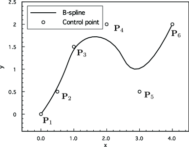
Figure 1: Example B-spline with associated control points.

• The curve requires a set of control points to be defined which may or may not lie on the curve

• The curve requires the definition of a knot vector, defined as a non-decreasing sequence of coordinates in the parameter space, which in this case is given by $\Xi=\{0,0,0,1,2,3,4,4,4\}$

• In this instance the curve is constructed from an open knot vector which results in a spline that is interpolatory at the beginning and end of the curve.

• If knot values are repeated, then it is found that the order of continuity decreases at that point in the spline.

The knot vector is a concept which is often unfamilar to those working in the field of numerical analysis but should be considered carefully, since it has a large influence on the resulting spline. The most important aspect of the knot vector is the relative difference between the components and for this reason the values can be scaled if required. That is, the knot vector $\Xi=\{0,0,0,1,2,3,4,4,4\}$ with $\xi\in[0,4)$ is equivalent to $\Xi=\{0,0,0,0.1,0.2,0.3,0.4,0.4,0.4\}$ with $\xi\in[0,0.4)$. In later sections we will see that the process of applying refinement in IGABEM has a considerable effect on the knot vector. Knot vectors are ubiqutous in the fields of geometrical modelling and isogeometric analysis and therefore the reader should become accustomed to their use.

We now introduce some more formal definitions which are required for succint notation in later sections. Denoting the dimensionality of the problem as $\mathbb{R}^{d}$ ($d=2,3$), the following three items are required to define fully a B-spline:

• The curve degree, $p$, e.g. linear ($p=1$), quadratic ($p=2$)…

• A set of of $n$ control points $\mathbf{P}_{a}\in\mathbb{R}^{d}$ , $1\leq a\leq n$

• A knot vector $\Xi=\{\xi_{1},\,\xi_{2},\,...,\,\xi_{n+p+1}\}$

Figure 2: Linear B-spline $p=1$

Figure 3: Quadratic B-spline, $p=2$

Figure 4: Cubic B-spline, $p=3$

Figures 2 to 4 illustrate linear, quadratic and cubic B-splines with their associated control points. The knot vectors associated with each curve are $\{0,0,1,2,3,3\}$, $\{0,0,0,1,2,3,3,3\}$ and $\{0,0,0,0,1,2,3,3,3,3\}$ respectively. Each of these are found to be open knot vectors which denotes that they contain $p+1$ repeated components at the beginning and end of the knot vector. The fact that the curve is interpolatory at the beginning and end is a direct consequence of this. In all future examples used in this paper, it can be assumed that open knot vectors are used. Repeated knot components may also occur at points which are not located at the extremes with a consequence that the continuity of the curve is reduced at that point.

2.1.1 B-spline and NURBS basis functions

The previous section served as an overview of B-splines and some of the terminlogy associated with their construction. But for a B-spline to be completely defined, some attention must be paid towards their associated basis functions. The idea of interpolating a discrete number of points mirrors the technology seen in conventional FEMs and BEMs but with a distinct difference - the curve is not required to exhibit the Kronecker delta property at the interpolated points. The consequences of this are that when interpolating fields such as displacement, the value obtained at nodal points does not represent any real displacement but rather a coefficient used for interpolation. This is similar to meshless methods where techniques such as Lagrange multipliers [8] and the penalty method approach [3] are employed to impose essential boundary conditions.

Turning our attention towards B-spline basis functions, we introduce the following expression which fully describes a B-spline in terms of its basis functions and control points. This is written as

$$\mathbf{C}(\xi)=\sum_{a=1}^{n}N_{a,p}(\xi)\mathbf{P}_{a}$$ (1)

where $\mathbf{C}(\xi)$ is a vector denoting the Cartesian coordinates of the location described by the parametric coordinate $\xi$, and $N_{a,p}(\xi)$ denotes the set of B-spline basis functions of degree $p$ at $\xi$. The basis functions are defined as

$$N_{a,0}(\xi)=\begin{cases}1\quad&\textrm{if}\quad\xi_{a}\leq\xi<\xi_{a+1}\\ 0\quad&\textrm{otherwise}\end{cases}$$ (2)

and for $p=1,2,3...$

$$N_{a,p}(\xi)= \frac{\xi-\xi_{a}}{\xi_{a+p}-\xi_{a}}N_{a,p-1}(\xi)$$

$$+\frac{\xi_{a+p+1}-\xi}{\xi_{a+p+1}-\xi_{a+1}}N_{a+1,p-1}(\xi).$$ (3)

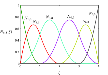
Figure 5: B-spline basis functions for curve shown in Fig. 4 and knot vector $\Xi=\{0,0,0,0,1,2,3,3,3,3\}$

Fig. 5 illustrates the basis functions corresponding to the B-spline shown in Fig. 1; here the interpolatory nature of the first and last basis functions is evident. What should be noted is that Eqns. (2) and (5) are recursive in nature and, in their current form, considerably more expensive than conventional polynomial basis function expressions. However, there exist several efficient computational algorithms for their evaluation such as the Cox-de-Boor algorithm[24],[26] and, more recently, the extraction operator [27]. B-spline derivatives are also required for numerical analysis, but the algorithms for determining their values are standard in CAD literature, with details given in A.1.

In CAD surface modelling packages, NURBS represent the dominant tool used to describe curves and surfaces where, in fact, they are found to be a superset of B-splines and only differ from their counterparts by the use of an additional coordinate often referred to as a ‘weighting’. In some interpretations NURBS are seen as a ‘projection’ of B-splines from a higher dimensional space (see [13]), and it can be shown that some attractive properties emerge. In particular, NURBS are able to reproduce circular arcs, spheres and conic sections exactly (cf. B-splines which only approximate such shapes) and this is achieved through the appropriate choice of weightings. Each control point $\mathbf{P}_{a}$ is associated with a weighting $w_{a}$ leading to a set of NURBS basis functions denoted by $R_{a,p}(\xi)$. The curve is then interpolated as

$$\mathbf{C}(\xi)=\sum_{a=1}^{n}R_{a,p}(\xi)\mathbf{P}_{a}$$ (4)

with the NURBS basis functions given by

$$R_{a,p}(\xi)=\frac{N_{a,p}(\xi)w_{a}}{\sum_{\hat{a}=1}^{n}N_{\hat{a},p}(\xi)w_{\hat{a}}}$$ (5)

where $N_{a,p}$ can be found from Eqns (2) and (3). In the case that the weights are all set to unity (i.e. $w_{a}=1\,\,\forall a$), the basis functions given by (5) reduce to the B-spline basis functions of (3). Expressions for the derivaties of NURBS basis functions can also be found, and are detailed in A.2. Since B-splines are a subset of NURBS, for the sake of generality, NURBS will be considered for all future examples.

Isogeometric analysis relies on the use of the basis functions outlined in this section and is conceptually very simple - we use the basis functions used to describe the geometry of the problem to approximate the unknown fields in the governing PDEs. That is, in the case of elastostatic analysis using BEM, the displacement and traction components are approximated using NURBS basis functions. The benefit of this approach is clear, since the task of producing a boundary discretisation (mesh) is completely provided by CAD and, once boundary conditions and material properties have been defined, analysis can be carried out immediately.

3 Conventional BEM

To illustrate the differences between conventional and isogeometric BEM implementations some details of standard BEM technology are presented here. The purpose of this section is not to give a complete derivation of the method but rather an overview to aid understanding in later sections. The interested reader is advised to consult standard BEM references for more details [12],[2],[15],[34]. In this section we describe the direct collocation form of the BEM using piecewise polynomial shape functions; the indirect form of the BEM and the Galerkin BEM are not described, though there appears to be no reason why the Galerkin BEM cannot be developed in an isogeometric framework.

To begin, we define the domain of the problem $\Omega$ with boundary $\Gamma=\partial\Omega$. We also define two points $\mathbf{x^{\prime}}$ and $\mathbf{x}$, commonly referred to as the source point and field point respectively, these points being separated by a distance $r$ given by the Euclidean norm

Figure 6: Definition of problem domain with source and field points.

$$r:=||\mathbf{x^{\prime}}-\mathbf{x}||$$ (6)

(see Fig. 6). The point $\mathbf{x^{\prime}}$ is often referred to as the collocation point, since in the conventional collocation BEM implementation, the system of equations is constructed by taking the collocation point to lie at each nodal point in turn. The field point $\mathbf{x}$ represents any sampling point, considered in a numerical integration scheme, on the portion of boundary over which integration is performed. Making the assumption of linear elasticity and in the absence of body forces, we can write the displacement boundary integral equation (DBIE) which relates displacements and tractions around the boundary $\Gamma$,

$$C_{ij}(\mathbf{x}^{\prime}) u_{j}(\mathbf{x}^{\prime})+\mathchoice{{\vbox{\hbox{$\textstyle-$}}\kern-4.86108pt}}{{\vbox{\hbox{$\scriptstyle-$}}\kern-3.25pt}}{{\vbox{\hbox{$\scriptscriptstyle-$}}\kern-2.29166pt}}{{\vbox{\hbox{$\scriptscriptstyle-$}}\kern-1.875pt}}\!\int_{\Gamma}T_{ij}(\mathbf{x}^{\prime},\mathbf{x})u_{j}(\mathbf{x})\,\mathrm{d}\Gamma(\mathbf{x})$$

$$=\int_{\Gamma}U_{ij}(\mathbf{x}^{\prime},\mathbf{x})t_{j}(\mathbf{x})\,\mathrm{d}\Gamma(\mathbf{x})\quad i,j=1,2$$ (7)

where $C_{ij}$ is a jump term that arises from the limiting process of the boundary integral on the left hand side of (7) and is dependent on the geometry at the source point, $u_{j}$ and $t_{j}$ are the components of displacement and traction around the boundary and $U_{ij}$ and $T_{ij}$ are displacement and traction fundamental solutions relating to a source point direction component $i$ and field point component $j$. These fundamental solutions for 2D linear elasticity may be found in Appendix B.1.

In its current form, Eq. (7) is not amenable for numerical implementation since $u_{j}$ and $t_{j}$ represent unknown continuous fields. We therefore proceed in the usual fashion of discretisation by splitting the boundary of the problem into elements with local coordinate $\eta\in[-1,1]$ over which the geometry and fields can be approximated as

$$\mathbf{x}_{e}(\eta) =\sum_{b=1}^{n_{b}}N_{b}(\eta)\mathbf{x}_{b}$$ (8)

$$\mathbf{u}_{e}(\eta) =\sum_{b=1}^{n_{b}}N_{b}(\eta)\mathbf{u}_{b}$$ (9)

$$\mathbf{t}_{e}(\eta) =\sum_{b=1}^{n_{b}}N_{b}(\eta)\mathbf{t}_{b}$$ (10)

Figure 7: Continuous quadratic basis functions

where $n_{b}$ is the number of local basis functions (eg. $b=3$ for a quadratic element), $N_{b}(\eta)$ are the set of polynomial basis functions (see Fig. 7 for the commonly used quadratic Lagrangian basis functions) and $\mathbf{x}_{b}$, $\mathbf{u}_{b}$, $\mathbf{t}_{b}$ are vectors of nodal coordinates, displacements and tractions respectively. The subscript $e$ has been used in Eqns (8) to (10) to denote that the vectors apply to a specific element $e$. By inserting Eqns (9) and (10) into (7), the discretised DBIE can be written as

$$C_{ij}(\mathbf{x^{\prime}})u_{j}(\mathbf{x^{\prime}})$$

$$+\sum_{e=1}^{N_{e}}\sum_{b=1}^{n_{b}}\left[\int_{-1}^{+1}T_{ij}(\mathbf{x^{\prime}},\mathbf{x}(\eta))N_{b}(\eta)J^{e}(\eta)\,\mathrm{d}\eta\right]\,u_{j}^{eb}$$

$$=\sum_{e=1}^{N_{e}}\sum_{b=1}^{n_{b}}\left[\int_{-1}^{+1}U_{ij}(\mathbf{x^{\prime}},\mathbf{x}(\eta))N_{b}(\eta)J^{e}(\eta)\,\mathrm{d}\eta\right]\,t_{j}^{eb}.$$ (11)

where $J^{e}(\eta)$ represents the Jacobian of transformation for element $e$ that maps $\eta\to\Gamma$ and $1\leq e\leq N_{e}$ is the set of element numbers.

As mentioned previously, the system of equations is formed by considering the collocation point $\mathbf{x^{\prime}}$ to lie at each nodal point in turn. In this way, a set of matrices are assembled relating all displacement components and traction components. This set of equations can be written as

$$\mathbf{H}\mathbf{u}=\mathbf{G}\mathbf{t}$$ (12)

with the square matrix $\mathbf{H}$ containing all integrals of the $T_{ij}$ kernel plus the jump terms $C_{ij}$, the rectangular matrix $\mathbf{G}$ containing all integrals of the $U_{ij}$ kernel, and the vectors $\mathbf{u}$, $\mathbf{t}$ containing nodal displacement and traction components respectively. By prescribing a suitable set of boundary conditions, which may consist of a set of displacements and tractions, equation (12) may be rearranged to give a set of linear equations in the form

$$\mathbf{A}\mathbf{x}=\mathbf{b},$$ (13)

where $\mathbf{x}$ represents the vector of unknown degrees of freedom. The linear system (13) can be solved for $\mathbf{x}$ using conventional or fast solvers [9, 25] while noting that $\mathbf{A}$ is a full, non-symmetric matrix.

4 Isogeometric BEM

Our attention now focuses on the main idea of the paper: presenting the isogeometric boundary element method implementation for 2D elastostatic analysis. However, before more details are given, a comment should be made on the key difference of IGABEM over conventional BEM. Essentially, it can be reduced to the use of NURBS basis functions in place of the conventional polynomial counterparts. There are certain consequences for implementation when NURBS basis functions are used (such as dealing with nodal points which no longer lie on the boundary), but this key concept should be kept in mind throughout the following sections.

We begin by considering a simple 2D geometry of a nuclear reactor vessel; symmetry has been exploited to simplify the problem. The exact geometry can be described using the NURBS as illustrated in Fig. 8. All information necessary to define the NURBS curve is provided by a CAD model. In this example we have chosen, for the entire boundary, to use quadratic basis functions ($p=2$) which are illustrated in Fig. 9 .

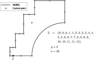
Figure 8: Control points and NURBS curve definition for reactor problem. Appendix C details the control point coordinates and weights.

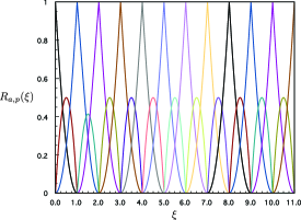
Figure 9: NURBS basis functions for reactor problem.

4.1 Element definition

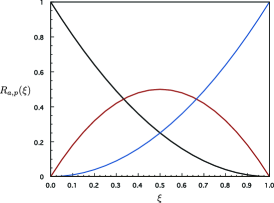
Figure 10: NURBS basis functions for first element of reactor problem.

As shown in Sec. 3, the boundary integrals in the DBIE are evaluated over the entire domain by summing all elemental contributions. But for IGABEM, it is not immediately obvious what our definition of elements should be. However, we should bear in mind that some notion of ‘elements’ is used in IGABEM simply as a construct for numerical integration, and this is the definition used in the remainder of this paper. The element domain is required to cover only the portion of the boundary where the relevant basis functions are non-zero. For convenience this leads us to a definition of element boundaries as the unique values of the knot vector, which can be implemented simply as

uniqueKnots = unique(knotVec);
elRanges = [uniqueKnots(1:end-1)’ uniqueKnots(2:end)’];

For example, the first element for the reactor problem is defined by $\xi\in[0,1]$ with the set of non-zero basis functions over this element illustrated in Fig. 10.

For the purposes of numerical integration using Gauss-Legendre quadrature, local coordinates in the range $[-1,1]$ over a particular element are most commonly used, so a transformation that maps from the parameter space $\xi\in[\xi_{1},\xi_{a+p+1}]$ to a parent coordinate space defined over an element as $\hat{\xi}\in[-1,1]$ is required. To achieve this, a Jacobian of transformation is used which comprises two terms combined in the chain rule sense: a mapping from the physical coordinate space to parameter space ($d\Gamma/d\xi$) and a mapping from parameter space to the local parent coordinate space ($d\xi/d\hat{\xi}$). This results in the following Jacobian of transformation:

$$J(\hat{\xi})=\frac{d\Gamma}{d\hat{\xi}}=\frac{d\Gamma}{d\xi}\frac{d\xi}{d\hat{\xi}}$$ (14)

Explicit expressions for the derivatives on the right hand side of Eq. (14) are given in Appendix B.2.2.

4.1.1 Element connectivity

Before approximations of the geometry and unknown fields can be given, the non-zero basis functions must be determined for a particular element, thus forming a connectivity function. If this is done, then a set of local basis functions that are related to the global basis functions can be defined as

$$N_{b}^{e}(\hat{\xi})\equiv R_{a,p}(\xi(\hat{\xi}))$$ (15)

where the local basis function number $b$, element number $e$ and global basis function number are related by

$$a=conn(e,b)$$ (16)

where $conn()$ is a connectivity function. The connectivity function for the reactor problem is given in Appendix C.2. Using this definition of local basis functions, it is now possible to state isogeometric approximations for the geometry, displacement and traction as follows:

$$\mathbf{x}_{e}(\hat{\xi}) =\sum_{b=1}^{p+1}N_{b}^{e}(\hat{\xi})\mathbf{x}_{b}$$ (17)

$$\mathbf{u}_{e}(\hat{\xi}) =\sum_{b=1}^{p+1}N_{b}^{e}(\hat{\xi})\mathbf{d}_{b}$$ (18)

$$\mathbf{t}_{e}(\hat{\xi}) =\sum_{b=1}^{p+1}N_{b}^{e}(\hat{\xi})\mathbf{q}_{b}$$ (19)

where $\mathbf{x}_{b}$, $\mathbf{d}_{b}$ and $\mathbf{q}_{b}$ are vectors of the geometric coordinates, displacement coefficients and traction coefficients respectively, associated with the control point corresponding to the basis function $b$. It should be noted that we have used the term coefficient since the NURBS basis functions do not necessarily obey the Kronecker-delta property (in contrast to the polynomial basis functions shown in Fig. 7). Therefore, the terms $\mathbf{d}_{b}$ and $\mathbf{q}_{b}$ do not necessarily represent real displacements and tractions.

Is it is now a simple case of substituting Eqns (18) and (19) into the DBIE of (7) while using the Jacobian given by (14). This results in the following discretised equation for IGABEM:

$$C_{ij} (\mathbf{x^{\prime}})\sum_{l=1}^{p+1}N_{l}^{\bar{e}}(\hat{\xi}^{\prime})d_{j}^{l\bar{e}}$$

$$+\sum_{e=1}^{N_{e}}\sum_{l=1}^{p+1}\left[\int_{-1}^{+1}T_{ij}(\mathbf{x^{\prime}},\mathbf{x(\hat{\xi})})N_{l}^{e}(\hat{\xi})J(\hat{\xi})\,\mathrm{d}\hat{\xi}\right]\,d_{j}^{le}$$

$$=\sum_{e=1}^{N_{e}}\sum_{l=1}^{p+1}\left[\int_{-1}^{+1}U_{ij}(\mathbf{x^{\prime}},\mathbf{x(\hat{\xi})})N_{l}^{e}(\hat{\xi})J(\hat{\xi})\,\mathrm{d}\hat{\xi}\right]\,q_{j}^{le}.$$ (20)

where $d_{j}^{le}$ and $q_{j}^{le}$ represent components of the vectors $\mathbf{d}_{b}$ and $\mathbf{q}_{b}$ for the element $e$. We denote $\bar{e}$ as the element containing the collocation point $\mathbf{x}^{\prime}$ and $\hat{\xi}^{\prime}$ is the local coordinate of the collocation point in element $\bar{e}$. The reason for specifiying these terms concerns the term $u_{j}(\mathbf{x^{\prime}})$ as seen in Eq. (3). In the conventional implementation where collocation occurs at nodal points, the Kronecker-delta property of the basis functions ensures that at the collocation point itself the basis functions are interpolatory. In contrast to this, the IGABEM formulation cannot guarantee that this is true and the displacement must be interpolated as $u_{j}(\mathbf{x^{\prime}})=\sum_{l=1}^{p+1}N_{l}^{\bar{e}}(\hat{\xi}^{\prime})d_{j}^{l\bar{e}}$.

4.2 Collocation point definition

A significant change in IGABEM over conventional BEM is in the location of collocation points, since the normal practice of collocation at nodal positions is no longer valid. We can easily see why this is the case by inspecting the position of the control points in Fig. 8; it is evident that there is one control point in this example that does not lie on the boundary. Indeed, for most curved boundaries the control points will not lie on the boundary. Since the control points can be interpreted as nodes in the IGABEM formulation, this presents a problem since it is essential that collocation takes place on the boundary $\Gamma$. To overcome this, we choose to use the Greville abscissae definition [17], [20] to define the position of collocation points in parameter space. This is defined as:

$$\xi_{a}^{\prime}=\frac{\xi_{a+1}+\xi_{a+2}+\cdots+\xi_{a+p}}{p}\quad a=1,2,\cdots,n$$ (21)

In Matlab® , this is easily evaluated as:

collocPts = zeros(1,n);
for i=1:n
   collocPts(i) = sum(knotVec(i+1:i+p)) / p;
end

where n denotes the number of control points, p is the curve order and knotVec is the knot vector.

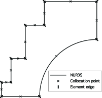
Figure 11: Collocation point and element definitions for reactor problem.

If this definition is applied to the geometry of the reactor vessel, then the collocation points are as shown in Fig. 11. The coordinates in physical space can be found by using (1) with the NURBS basis functions given by (5). The definition of the element boundaries is also illustrated in this figure.

4.3 Implementation aspects

The previous two sections outlining the definition of boundary elements and collocation points within an isogeometric BEM framework specify the key aspects that must be changed for an existing collocation BEM implementation. Our attention now focuses on the implementation for the reactor vessel problem to illustrate these aspects.

4.3.1 Refinement

The discretisation in Fig. 8 represents the geometry of the reactor problem exactly, but experienced analysts will be acutely aware that, although the geometry may be captured, the basis functions may be insufficient to capture the gradients in the unknown fields, consequently leading to large errors in the solution. This leads to one of the most beneficial properties of B-splines and NURBS for numerical analysis, which is that the mesh can be refined to arrive at a richer set of basis functions while preserving the exact geometry at all stages. In the current paper we present two types of refinement: knot insertion and order elevation, termed h-refinement and p-refinement in numerical analysis literature. The algorithms for these refinement processes are standard in CAD, with details given in [24],[26] and source code given in [1].

We can illustrate both knot insertion and order elevation using the reactor problem shown in Fig. 8. Figs 12 and 13 illustrate knot insertion where additional knots have been inserted uniformly into the original knot vector. Figs 14 and 15 illustrate order elevation where the basis functions have been increased from quadratic ($p=2$) to cubic ($p=3$). Both types of refinement introduce changes to the knot vector and set of control points. A third type of refinement which is often referred to as k-refinement can also be considered which is a combination of p- and h- refinement. It arises due to the non-commutative nature of the aforementioned refinements. k-refinement is not considered in the present paper.

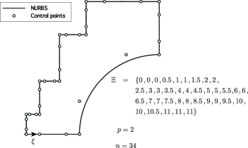
Figure 12: Control points and NURBS curve definition for reactor problem after knot insertion.

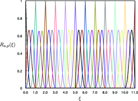
Figure 13: NURBS basis functions for reactor problem after uniform knot insertion (h-refinment)

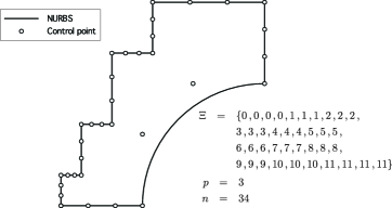
Figure 14: Control points and NURBS curve for reactor problem after order elevation

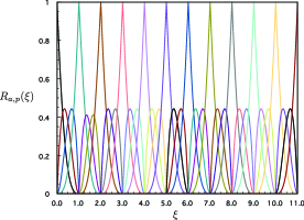
Figure 15: NURBS basis functions for reactor problem after order elevation

4.3.2 Integration

A key feature of any BEM implementation is the evaluation of the boundary integrals containing the kernels over element domains. It is well-known that both regular and singular integrands are found depending on the position of the collocation point relative to the field element. Essentially, the evaluation of BEM integrals is split into three different types described as

1. Regular integration: the collocation point lies in an element different from the field element.

2. Nearly singular integration: the collocation point lies in a element not on but near the field element.

3. Singular integration: the collocation point lies in the field element and can be one of two types:

   Strongly singular integrals: ($T_{ij}$ kernel, $\mathcal{O}(1/r)$ in 2D)

   Weakly singular integrals: ($U_{ij}$ kernel, $\mathcal{O}(\ln(1/r))$ in 2D)

In the present study, we choose to treat the regular and nearly-singular integrals in the same manner, although several methods exists for the efficient treatment of integrals of the latter type [32],[21],[16]. The evaluation of singular integrals must be given close consideration since they are found to have a large influence on the accuracy of the resulting solution.

The present work uses the subtraction of singularity method (SST) [18] to evaluate strongly singular integrals, in which the integrand is split into its regular and singular parts. Further details of the method are shown in [29] with a full implementation given in [1]. The idea is to separate the integral into a regular part (which can evaluated using standard quadrature routines) and a singular part which can be evaluated analytically (for 2D boundary integrals). If the SST method is used, however, the jump term $C_{ij}$ must be calculated explicitly (c.f. the rigid body motion technique [15] which calculates it implicitly). However, a simple formula exists [18] for the 2D case which is restated here as

$$C=\frac{1}{8\pi(1-\bar{\nu})}\left[\begin{array}[]{cc}\begin{array}[]{l}4(1-\bar{\nu})(\theta_{1}-\theta_{2})\\ \phantom{a}+(\sin 2\theta_{1}-\sin 2\theta_{2})\end{array}&\cos 2\theta_{2}-\cos 2\theta_{1}\\ \cos 2\theta_{2}-\cos 2\theta_{1}&\begin{array}[]{l}4(1-\bar{\nu})(\theta_{1}-\theta_{2})\\ \phantom{a}-(\sin 2\theta_{1}-\sin 2\theta_{2})\end{array}\end{array}\right]$$ (22)

where $\bar{\nu}=\nu$ for plane strain and $\bar{\nu}=\nu/(1+\nu)$ for plane stress and the angles $\theta_{1}$, $\theta_{2}$ are related to the normals of the surface at the collocation point (see Fig.2 in [18]).

For weakly singular integrals, a variety of techniques are available including specific logarithmic quadrature points and weights [30], but in the present study we choose to use the Telles transformation [32] which cancels the singularity leaving a regular integrand. This is achieved through the following transformation:

$$\hat{\xi}=\frac{(\gamma-\gamma^{\prime})^{3}+\gamma^{\prime}(\gamma^{\prime 2}+3)}{(1+3\gamma^{\prime 2})}$$ (23)

where

$$\gamma^{\prime}=\sqrt[3]{\hat{\xi}^{\prime}(\hat{\xi}^{\prime 2}-1)+|\hat{\xi}^{\prime 2}-1|}+\sqrt[3]{\hat{\xi}^{\prime}(\hat{\xi}^{\prime 2}-1)-|\hat{\xi}^{\prime 2}-1|+\hat{\xi}^{\prime}}$$ (24)

$\xi^{\prime}$ denotes the location of the singularity in the parent space ($\xi^{\prime}\in[-1,1]$) and $\gamma$ represents the new integration variable. Therefore, a Jacobian which transforms from the parent space $\hat{\xi}\in[-1,1]$ to $\gamma$ is required. This is given as:

$$\mathrm{d}\hat{\xi}=\frac{3(\gamma-\gamma^{\prime})^{2}}{1+3\gamma^{\prime 2}}\mathrm{d}\gamma$$ (25)

Using Eqn. (23), (24) and (25), the transformation of the integration can be expressed as:

$$\int_{-1}^{+1}f(\hat{\xi})\mathrm{d}\hat{\xi}=\int_{-1}^{+1}f\left[\frac{(\gamma-\gamma^{\prime})^{3}+\gamma^{\prime}(\gamma^{\prime 2}+3)}{(1+3\gamma^{\prime 2})}\right]\frac{3(\gamma-\gamma^{\prime})^{2}}{1+3\gamma^{\prime 2}}\mathrm{d}\gamma$$ (26)

A derivation of the transformation is given completely in [32] with a full implementation for the $U_{ij}$ kernels given in [1].

4.3.3 IGABEM algorithm

Now that the integration routines which form the core of IGABEM implementation have been outlined, we are in a position to give an overview of the entire IGABEM algorithm, illustrated in Algorithm 1.

Algorithm 1 IGABEM algorithm

1:Read CAD input data $\triangleright$ e.g. Control points, knot vector

2:Read material properties, boundary conditions

3:Perform mesh refinement $\triangleright$ e.g. knot insertion or order elevation

4:

5:for $c\leftarrow 1,n_{c}$ do$\triangleright$ Loop over collocation pts

6:     $jumpTerm\leftarrow calcJumpTerm(collocNormals(c))$ $\triangleright$ Calculate $C_{ij}$

7:     for $e\leftarrow 1,n_{el}$ do$\triangleright$ Loop over elements

8:         $elementConn\leftarrow glbConn(e)$$\triangleright$ Element connectivity

9:         $elRange\leftarrow ElmtRanges(e)$$\triangleright$ Range of element

10:

11:         if $c\in elRange$ then$\triangleright$ Singular integration

12:              $\mathbf{H}_{sub}\leftarrow SSTIntegration(c,e,C_{ij})$ $\triangleright$ SST integration

13:              $\mathbf{G}_{sub}\leftarrow TellesIntegration(c,e)$ $\triangleright$ Telles transformation

14:         else$\triangleright$ Non-singular integration

15:              $[\mathbf{H}_{sub},\mathbf{G}_{sub}]\leftarrow GaussLegendreQuad(c,e)$

16:         end if

17:

18:         $\mathbf{H}(c,elementConn)\leftarrow\mathbf{H}_{sub}$ $\triangleright$ Add submatrix to global $\mathbf{H}$ matrix

19:         $\mathbf{G}(c,elementConn)\leftarrow\mathbf{G}_{sub}$ $\triangleright$ Add submatrix to global $\mathbf{G}$ matrix

20:     end for

21:end for

22:

23:$\triangleright$ Apply boundary conditions

24:$[\mathbf{A},\mathbf{z}]\leftarrow applyBoundConds(\mathbf{H},\mathbf{G})$

25:$\mathbf{x}\leftarrow solve(\mathbf{A},\mathbf{z})$ $\triangleright$ Solve system of equations

In this algorithm the $\mathbf{H}$ and $\mathbf{G}$ matrices have been calculated explicitly before boundary conditions are applied to arrive at the final system of equations. For efficiency, commercial BEM implementations often calculate $\mathbf{A}$ and $\mathbf{z}$ directly, thereby making the construction of the $\mathbf{H}$ and $\mathbf{G}$ matrices redundant.

4.4 Example

Finally, an example problem using the geometry of the reactor used throughout the current paper is defined and analysed. The problem geometry, boundary conditions and material properties are shown in Fig. 16 where symmetrical boundary conditions are applied at $x=100$ and $y=0$, and a constant pressure is exerted on the inner boundary. Plane strain is assumed.

By applying knot insertion to the original mesh shown in Fig. 11, the discretisation shown in Fig. 17 was used to perform the IGABEM analysis. The results are shown in Fig. 18 by plotting the exaggerated displacement profile with FEM results also plotted for comparison. As can be seen, excellent agreement is obtained. In addition, a convergence study was carried out to assess the accuracy of IGABEM over a standard BEM implementation with quadratic basis functions. Using h-refinement in both methods, the $L_{2}$ norm in displacement was calculated for each mesh as:

$$||\mathbf{u}||_{L_{2}}=\sqrt{\int_{\Gamma}\sum_{i=1}^{d}(u_{i})^{2}\,\mathrm{d}\Gamma}$$ (27)

The results obtained are shown in Fig. 19 where a significant improvement in accuracy over the standard BEM implementation can be seen. The reference solution corresponds to the converged result of a BEM analysis using quadratic basis functions.

Figure 16: Definition of nuclear reactor geometry, boundary conditions and material properties.

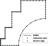
Figure 17: Mesh used for reactor problem IGABEM analysis detailing element edges and collocation point positions.

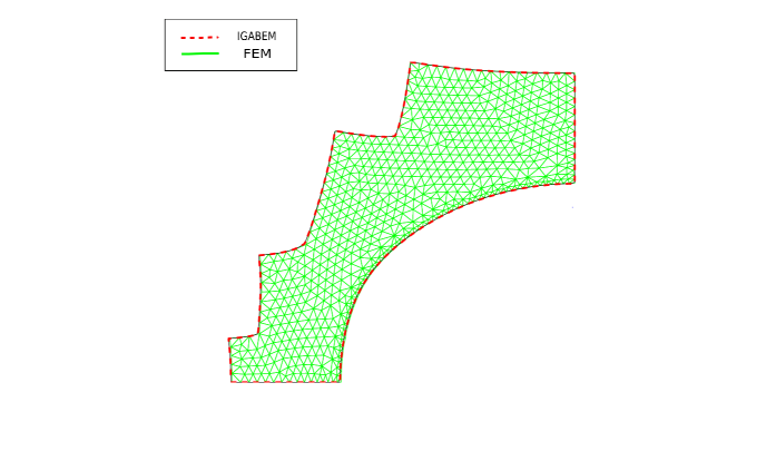
Figure 18: Comparison of IGABEM and FEM results for reactor problem - exaggerated displacement profile.

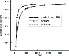
Figure 19: Comparison of $L_{2}$ displacement norms for reactor problem using IGABEM and standard BEM with quadratic basis functions.

5 Conclusions

The implementation aspects of an isogeometric BEM were outlined, with attention paid to areas which differ from a conventional BEM implementation. What is evident is that IGABEM present a particularly attractive approach for analysis, since the data provided by CAD can be used directly without the need to create a mesh. In addition, refinement schemes were outlined which provide more refinement or richer basis functions in required areas. Finally, an example was used to illustrate the simplicity and accuracy of the method where it was shown that good aggrement with FEM was obtained, and in addition, significant improvements in accuracy over a standard BEM implementation with quadratic basis functions were demonstrated.

Appendix A B-splines/NURBS

A.1 B-spline derivatives

The first order derivative of the B-spline basis function is expressed as

$$\frac{d}{d\xi}N_{a,p}(\xi)=\frac{p}{\xi_{a+p}-\xi_{a}}N_{a,p-1}(\xi)-\frac{p}{\xi_{a+p+1}-\xi_{a+1}}N_{a+1,p-1}(\xi).$$ (28)

where $p$ is the polynomial order, $a$ the basis function index. The higher order derivatives can be obtained by differentiating the two sides of equation (28):

$$\frac{d^{k}}{d^{k}\xi}N_{a,p}(\xi)=\frac{p}{\xi_{a+p}-\xi_{a}}\left(\frac{d^{k-1}}{d^{k-1}\xi}N_{a,p-1}(\xi)\right)-\frac{p}{\xi_{a+p+1}-\xi_{a+1}}\left(\frac{d^{k-1}}{d^{k-1}\xi}N_{a+1,p-1}(\xi)\right).$$ (29)

From Eqn (28) and (29), we can express high order derivatives with $N_{a,p-k},\cdots,N_{a+k,p-k}$:

$$\frac{d^{k}}{d^{k}\xi}N_{a,p}(\xi)=\frac{p!}{(p-k)!}\sum_{j=0}^{k}\alpha_{k,b}N_{a+b,p-k}(\xi),$$ (30)

with

$$\alpha_{0,0} =1,$$

$$\alpha_{k,0} =\frac{\alpha_{k-1,0}}{\xi_{a+p-k+1}-\xi_{a}},$$

$$\alpha_{k,b} =\frac{\alpha_{k-1,b}-\alpha_{k-1,b-1}}{\xi_{a+p+b-k+1}-\xi_{a+b}}\qquad b=1,\dots,k-1,$$

$$\alpha_{k,k} =\frac{-\alpha_{k-1,k-1}}{\xi_{a+p+1}-\xi_{a+k}}.$$

A.2 NURBS derivatives

From Eqn (5), we can give the first order derivative of NURBS basis function

$$\frac{d}{d\xi}R_{a}^{p}(\xi)=w_{a}\frac{W(\xi)N^{\prime}_{a,p}(\xi)-W^{\prime}(\xi)N_{a,p}(\xi)}{(W(\xi))^{2}},$$ (31)

where $N^{\prime}_{a,p}(\xi)\equiv\frac{d}{d\xi}N_{a,p}(\xi)$ and

$$W^{\prime}(\xi)=\sum_{\hat{a}=1}^{n}N^{\prime}_{\hat{a},p}(\xi)w_{\hat{a}}.$$ (32)

We introduce some notations for convenience

$$A_{a}^{(k)}(\xi)=w_{a}\frac{d^{k}}{d\xi^{k}}N_{a,p}(\xi),\qquad(\textrm{no sum on}\ i)$$ (33)

and

$$W^{(k)}(\xi)=\frac{d^{k}}{d\xi^{k}}W(\xi).$$ (34)

Then higher-order derivatives of these rational functions may be expressed in terms of lower-order derivatives as

$$\frac{d^{k}}{d\xi^{k}}R_{a}^{p}(\xi)=\frac{A_{a}^{(k)}(\xi)-\sum_{b=1}^{k}\binom{k}{b}W^{(b)}(\xi)\frac{d^{(k-b)}}{d\xi^{(k-b)}}R_{a}^{p}(\xi)}{W(\xi)},$$ (35)

where

$$\binom{k}{b}=\frac{k!}{b!(k-b)!}.$$ (36)

Appendix B BEM

B.1 2D Fundamental solutions

Denoting $\mu$ as the shear modulus, $\nu$ as Poisson’s ratio, $\delta_{ij}$ as the kronecker-delta function defined by

$$\delta_{ij}=\begin{cases}&0\quad i\neq j\\ &1\quad i=j,\end{cases}$$ (37)

and noting that a comma denotes differentiation, the fundamental solutions for 2D linear elasticity are given by:

$$U_{ij}(\mathbf{x}^{\prime},\mathbf{x})=\frac{1}{8\pi\mu(1-\nu)}\left\{(3-4\nu)\ln\left(\frac{1}{r}\right)\delta_{ij}+r_{,i}r_{,j}\right\}$$ (38)

$$T_{ij}(\mathbf{x}^{\prime},\mathbf{x})=\frac{-1}{4\pi(1-\nu)r}\left\{\frac{\partial r}{\partial n}[(1-2\nu)\delta_{ij}+2r_{,i}r_{,j}]-(1-2\nu)(r_{,i}n_{j}-r_{,j}n_{i})\right\}$$ (39)

B.2 Boundary element integration parameters

B.2.1 Normals

The normals can be calculated by:

$$n_{x}=\frac{1}{J(\xi)}\left[\frac{\mathrm{d}y(\xi)}{\mathrm{d}\xi}\right],$$ (40)

$$n_{y}=\frac{1}{J(\xi)}\left[\frac{\mathrm{d}x(\xi)}{\mathrm{d}\xi}\right],$$ (41)

with

$$\frac{\mathrm{d}x(\xi)}{\mathrm{d}\xi}=\sum_{b=1}^{p+1}\frac{\mathrm{d}N_{b}(\xi)}{\mathrm{d}\xi}x_{b},$$ (42)

$$\frac{\mathrm{d}y(\xi)}{\mathrm{d}\xi}=\sum_{b=1}^{p+1}\frac{\mathrm{d}N_{b}(\xi)}{\mathrm{d}\xi}y_{b}.$$ (43)

B.2.2 Jacobian of transformation

$$\frac{\mathrm{d}\xi(\hat{\xi})}{\mathrm{d}\hat{\xi}}=\frac{\xi_{f}-\xi_{s}}{2},$$ (44)

where $\xi_{s}$ and $\xi_{f}$ denotes the values of knots at the beginning and end of the element respectively (assuming an outward pointing normal).

$$\frac{\mathrm{d}\Gamma}{\mathrm{d}\xi}=\sqrt{\left(\frac{\mathrm{d}x(\xi)}{\mathrm{d}\xi}\right)^{2}+\left(\frac{\mathrm{d}y(\xi)}{\mathrm{d}\xi}\right)^{2}}.\\$$ (45)

Appendix C Reactor problem data

C.1 Control points and weights

index ($a$)	Control point coordinate ($\mathbf{P}_{a}$)	Weight $w_{a}$
1	(0, 0)	1
2	(20, 0)	1
3	(40, 0)	1
4	(40, 60)	$\sqrt{2}/2$
5	(100, 60)	1
6	(100, 80)	1
7	(100, 100)	1
8	(72.5, 100)	1
9	(45, 100)	1
10	(45, 87.5)	1
11	(45, 75)	1
12	(35, 75)	1
13	(25, 75)	1
14	(25, 57.5)	1
15	(25, 40)	1
16	(17.5, 40)	1
17	(10, 40)	1
18	(10, 27.5)	1
19	(10, 15)	1
20	(5, 15)	1
21	(0, 15)	1
22	(0, 7.5)	1
23	(0, 0)	1

C.2 Connectivity matrix

element index ($e$)	global basis index ($a$) for ($b_{1}$,$b_{2}$,$b_{3}$)
1	1, 2, 3
2	3, 4, 5
3	5, 6, 7
4	7, 8, 9
5	9, 10, 11
6	11, 12, 13
7	13, 14, 15
8	15, 16, 17
9	17, 18, 19
10	19, 20, 21
11	21, 22, 1

v

References

- [1] https://github.com/bobbiesimpson/isogeometric-bem, 2011.
- [2] M.H. Aliabadi. The boundary element method: applications in solids and structures. John Wiley and Sons, 2002.
- [3] T. Zhu amd S.N. Atluri. A modified collocation method and a penalty formulation for enforcing the essential boundary conditions in the element free galerkin method. Computational Mechanics, 21(3):211–222, 1998.
- [4] F. Auricchio, L.B. Da Veiga, T.J.R. Hughes, A. Reali, and G. Sangalli. Isogeometric collocation methods. Mathematical Models and Methods in Applied Sciences, 20(11):2075–2107, 2010.
- [5] Y. Bazilevs, V.M. Calo, J.A. Cottrell, J.A. Evans, T.J.R. Hughes, S. Lipton, M.A. Scott, and T.W. Sederberg. Isogeometric analysis using T-splines. Computer Methods in Applied Mechanics and Engineering, 199(5-8):229–263, 2010.
- [6] Y. Bazilevs, V.M. Calo, T.J.R. Hughes, and Y. Zhang. Isogeometric fluid-structure interaction: theory, algorithms, and computations. Computational Mechanics, 43(1):3–37, 2008.
- [7] Y. Bazilevs, J.R. Gohean, T.J.R. Hughes, R.D. Moser, and Y. Zhang. Patient-specific isogeometric fluid-structure interaction analysis of thoracic aortic blood flow due to implantation of the jarvik 2000 left ventricular assist device. Computer Methods in Applied Mechanics and Engineering, 198(45-46):3534–3550, 2009.
- [8] T. Belytschko, Y.Y. Lu, and G. Gu. Element free galerkin methods. International Journal for Numerical Methods in Engineering, 37(2):229–256, 1994.
- [9] I. Benedetti, M. H. Aliabadi, and G. Davi. A fast 3d dual boundary element. method based on hierarchical matrices. International journal of solids and structures, 45(7-8):2355–2376, 2008.
- [10] D.J. Benson, Y. Bazilevs, M.C. Hsu, and T.J.R. Hughes. Isogeometric shell analysis: The reissner-mindlin shell. Computer Methods in Applied Mechanics and Engineering, 199(5-8):276–289, 2010.
- [11] D.J. Benson, Y. Bazilevs, E. De Luycker, M.-C. Hsu, M. Scott, T.J.R. Hughes, and T Belytschko. A generalized finite element formulation for arbitrary basis functions: From isogeometric analysis to xfem. International Journal for Numerical Methods in Engineering, 83(6):765–785, 2010.
- [12] C.A. Brebbia and J. Dominguez. Boundary elements: An introductory course. WIT press, 1992.
- [13] J.A. Cottrell, T.J.R. Hughes, and Y. Bazilevs. Isogeometric analysis: Toward integration of CAD and FEA. John Wiley and Sons, 2009.
- [14] J.A. Cottrell, A. Reali, Y. Bazilevs, and T.J.R. Hughes. Isogeometric analysis of structural vibrations. Computer Methods in Applied Mechanics and Engineering, 195(41-43):5257–5296, 2006.
- [15] T. Cruse. Numerical solutions in three dimensional elastostatics. International journal of solids and structures, 5:1259–1274, 1969.
- [16] T.A. Cruse and R. Aitha. Non-singular boundary integral equation implementation. International Journal for Numerical Methods in Engineering, 36:237–254, 1993.
- [17] T. Greville. Numerical procedures for interpolation by spline functions. Journal of the Society for Industrial and Applied Mathematics: Series B, Numerical Analysis, 1964.
- [18] M. Guiggiani and P. Casalini. Direct computation of Cauchy Principal Value integrals in advanced boundary elements. International Journal for Numerical Methods in Engineering, 24:1711–1720, 1987.
- [19] T.J.R. Hughes, J.A. Cottrell, and Y. Bazilevs. Isogeometric analysis: CAD, finite elements, NURBS, exact geometry and mesh refinement. Computer Methods in Applied Mechanics and Engineering, 194(39-41):4135–4195, 2005.
- [20] R. Johnson. Higher order B-spline collocation at the Greville abscissae. Applied Numerical Mathematics, 52:63–75, 2005.
- [21] J.C. Lachat and J.O. Watson. Effective numerical treatment of boundary integral equations: a formulaton for elastostatics. International Journal for Numerical Methods in Engineering, 10:991–1005, 1976.
- [22] J. Lu. Isogeometric contact analysis: Geometric basis and formulation for frictionless contact. Computer Methods in Applied Mechanics and Engineering, 200:726–741, 2011.
- [23] N. Nguyen-Thanh, H. Nguyen-Xuan, S.P.A. Bordas, and T. Rabczuk. Isogeometric analysis using polynomial splines over hierarchical T-meshes for two-dimensional elastic solids. Computer Methods in Applied Mechanics and Engineering, 200:1892–1908, 2011.
- [24] L. Piegl and W. Tiller. The NURBS book. Springer, 1995.
- [25] V. Popov and H. Power. An O(N) taylor series multipole boundary element method for three-dimensional elasticity problems. Engineering analysis with boundary elements, 25(1):7–18, 2001.
- [26] D.F. Rogers. An introduction to NURBS: with historical perspective. Elsevier, 2001.
- [27] Michael A. Scott, Michael J. Borden, Clemens V. Verhoosel, Thomas W. Sederberg, and Thomas J. R. Hughes. Isogeometric finite element data structures based on bézier extraction of t-splines. International Journal for Numerical Methods in Engineering, 88:126–156, 2011.
- [28] R.N. Simpson, S.P.A. Bordas, J. Trevelyan, and T. Rabczuk. A two-dimensional isogeometric boundary element method for elastostatic analysis. Computer Methods in Applied Mechanics and Engineering (in press), 2011.
- [29] V. Sladek and J. Sladek. Singular integrals in boundary element methods. Computational Mechanics Publications, 1998.
- [30] A.H. Stroud and D. Secrest. Gaussian quadrature formulas. Prentice-Hall, New York, 1966.
- [31] R.L. Taylor. Isogeometric analysis of nearly incompressible solids. International Journal for Numerical Methods in Engineering, 87:273–288, 2011.
- [32] J.C.F. Telles. A self-adaptive co-ordinate transformation for efficient numerical evaluation of general boundary integrals. International Journal for Numerical Methods in Engineering, 24(959-973), 1987.
- [33] C.V. Verhoosel, M.A. Scott, R. de Borst, and T.J.R. Hughes. An isogeometric approach to cohesive zone modeling. International Journal for Numerical Methods in Engineering, 87:336–360, 2011.
- [34] J.O. Watson. Advanced implementation of the boundary element method for two- and three-dimensional elastostatics. Applied Science Publishers, London, 1979.