Dynamic Memory Allocation Policies for
Postings in Real-Time Twitter Search

Abstract

We explore a real-time Twitter search application where tweets are arriving at a rate of several thousands per second. Real-time search demands that they be indexed and searchable immediately, which leads to a number of implementation challenges. In this paper, we focus on one aspect: dynamic postings allocation policies for index structures that are completely held in main memory. The core issue can be characterized as a “Goldilocks Problem”. Because memory remains today a scare resource, an allocation policy that is too aggressive leads to inefficient utilization, while a policy that is too conservative is slow and leads to fragmented postings lists. We present a dynamic postings allocation policy that allocates memory in increasingly-larger “slices” from a small number of large, fixed pools of memory. Through analytical models and experiments, we explore different settings that balance time (query evaluation speed) and space (memory utilization).

1 Introduction

The rise of social media and other forms of user-generated content challenges the traditional notion of search as operating on either static documents collections or document collections that evolve slowly enough where periodically running a batch indexer (e.g., every hour) suffices. We focus on real-time search in the context of Twitter: users demand to know what’s happening right now, especially in response to breaking news stories and other shared events such as hurricanes in the northeastern United States, the death of prominent figures, or televised political debates. For this, they often turn to real-time search.

The context of this study is Twitter’s Earlybird retrieval engine [2], which serves over two billion queries a day with an average query latency of 50 ms. Usually, tweets are searchable within 10 seconds after creation (most of the latency is from the processing pipeline—tweet indexing itself takes less than a millisecond). The service as a whole is of course a complex, distributed system with many components. In this paper, we focus on one aspect—dynamic memory allocation policies for postings allocation.

A key feature of Earlybird is that it incrementally indexes tweets as they are posted and makes them immediately searchable. The indexing process naturally requires allocating space for postings in a dynamic manner—we adopt a zero-copy approach that yields non-contiguous postings lists. The fundamental challenge boils down to a “Goldilocks Problem”, since memory today remains a scarce resource. A policy that is too aggressive in allocating memory for postings leads to inefficient utilization, because much of the allocated space will be empty. On the other hand, a policy that is too conservative slows the system, since memory allocation is a relatively costly operation and postings lists will become fragmented. Ideally, we’d like to strike a balance between the two extreme and find a “sweet spot” that balances speed with utilization.

We present a dynamic postings allocation policy that allocates increasingly-larger “slices” from a small number of memory pools. The production system, which we previously described in Busch et al. [2], deploys a particular instantiation of a general framework, which we articulate for the first time here. Until now, we have not thoroughly explored alternative parameter settings in a rigorous and controlled manner. Thus, the contribution of this paper is a detailed study of the design space for dynamic postings allocation in the context of our basic framework: we present both an analytical model for estimating time and space costs, which is subsequently validated by experiments on real data.

2 Operational Requirements

To set the stage, we begin by discussing differences and similarities between real-time search and “traditional” (e.g., web) search. First, two similarities:

• Low-latency, high-throughput query evaluation. Users are impatient and demand results quickly.

• In-memory indexes. The only practical way to achieve necessary performance requirements is to maintain all index structures in memory.

There are important differences as well:

• Immediate data availability. In real-time search, documents arrive rapidly, and users expect content to be searchable within seconds. This means that the indexer must achieve both low latency and high throughput. This requirement departs from common assumptions that indexing can be considered a batch operation. Although web crawlers achieve high throughput, it is generally not expected that crawled content be indexed immediately—an indexing delay of minutes to hours may be acceptable. This allows efficient indexing with batch processing frameworks such as MapReduce [7]. In contrast, real-time search demands that documents be searchable in seconds.

• Shared mutable state. A real-time search engine must handle shared mutable state in a multi-threaded execution environment with concurrent indexing and retrieval operations. In contrast, concurrency-related challenges are simpler to handle in web search: for example, it is possible to atomically “swap out” an old index with an updated new index without service disruption. Such a design would be impractical in real-time search.

• Dominance of the temporal signal. The nature of real-time search means that temporal signals are important for relevance ranking. This contrasts with web search, where document timestamps have a relatively minor role in determining relevance (news search being the obvious exception). This holds implications for how postings should be organized in index structures.

3 Baseline Architecture

Twitter’s production real-time search service is a complex distributed system spanning many machines, the details of which are beyond the scope of this paper. In this study, we specifically focus on Earlybird, which is the core retrieval engine. For the purposes of this paper, Earlybird receives boolean queries and returns tweets that satisfy the query, sorted in reverse chronological order. No relevance scoring is performed, which is, functionally speaking, handled by another component. Incoming tweets are hash partitioned across a number of replicated Earlybird instances, so that each individual instance serves a fraction of all tweets.

To understand our contributions, it is necessary to first provide some technical background. Here, we summarize material presented in a previous paper [2], but refer the reader to the original source for details.

3.1 Earlybird Overview

Earlybird is built on top of the open-source Lucene search engine and adapted to meet the demands of real-time search discussed in Section 2. The system is written completely in Java, primarily for three reasons: to take advantage of the existing Lucene Java codebase, to fit into Twitter’s JVM-centric development environment, and to take advantage of the easy-to-understand memory model for concurrency offered by Java and the JVM. Although this decision poses inherent challenges in terms of performance, with careful engineering and memory management we believe it is possible to build systems that are comparable in performance to those written in C/C++.

As with nearly all modern retrieval engines, Earlybird maintains an inverted index: postings are maintained in forward chronological order (most recent last) but are traversed backwards (most recent first); this is accomplished by maintaining a pointer to the current end of each postings list (more details in the next section).

Earlybird supports a full boolean query language consisting of conjunctions (ANDs), disjunctions (ORs), negations (NOTs), and phrase queries. Results are returned in reverse chronological order, i.e., most recent first. Boolean query evaluation is relatively straightforward, and in fact we use Lucene query operators “out of the box”, e.g., conjunctive queries correspond to postings intersections, disjunctive queries correspond to unions, and phrase queries correspond to intersections with positional constraints. Lucene provides an abstraction for postings lists and traversing postings—we provide an implementation for our custom indexes, and are able to reuse existing Lucene query evaluation code.

A particularly noteworthy aspect of Earlybird is the manner in which it handles shared mutable state (concurrent index reads and writes) using lightweight memory barriers. As this is not germane to the subject of this paper, we refer the reader elsewhere [2] for details. However, it is worth mentioning that the general strategy for handling concurrency is to limit the scope of data structures that hold shared mutable state. This is accomplished as follows: each instance of Earlybird manages multiple index segments (currently 12), and each segment holds a relatively small number of tweets (currently, $2^{23}\sim 8.4$ million tweets). Ingested tweets first fill up a segment before proceeding to the next one. Therefore, at any given time, there is at most one index segment actively being modified, whereas the remaining segments are read-only. Once an index segment ceases to accept new tweets, we can convert it from a write-friendly structure into an optimized and compressed read-only structure.

Due to this design, our paper is only concerned with the active index segment within an Earlybird instance: only for that index do we need to allocate memory for postings dynamically. This is described in more detail next.

3.2 Active Index Segment

As we argued in Section 2, the dominance of the temporal signal is a major distinguishing characteristic of real-time search, compared to traditional (web) search. The implication of this is that it would be desirable to traverse postings in reverse temporal order for query evaluation. Although this is not an absolute requirement, such a traversal order is the most convenient.

Following this reasoning further, it appears that existing approaches to index structure organization are not appropriate. The information retrieval literature discusses two types of indexes: document sorted and frequency/impact sorted. The latter seems unsuited for real-time search. What about document-sorted indexes? If we assign document ids to new tweets in ascending order, there are two obvious possibilities when indexing new documents:

First, we could append new postings to the ends of postings lists. However, this would require us to read postings backwards to achieve a reverse chronological traversal order. Unfortunately, this is not directly compatible with modern index compression techniques. Typically, document ids are converted into document gaps, or differences between consecutive document ids. These gaps are then compressed with integer coding techniques such as $\gamma$ codes, Rice codes, or PForDelta [18, 19]. It would be tricky for gap-based compression to support backwards traversal. Prefix-free codes ($\gamma$ and Rice codes) are meant to be decoded only in the forward direction. More recent techniques such as PForDelta are block-based, in that they code relatively large blocks of integers (e.g., 128 document ids) at a time. Reconciling this with the desire to have low-latency indexing would require additional complexity, although none of these issues are technically insurmountable.

Alternatively, we could prepend new postings to the beginnings of postings lists. This would allow us to read postings in the forward direction and preserve a reverse chronological traversal order. However, this presents memory management challenges, i.e., how would space for new postings be allocated? We are unaware of any work that has explored this strategy. Note that the naïve implementation using linked lists would be hopelessly inefficient: linked list traversal is slow due to the lack of reference locality and predictable memory access patterns. Furthermore, linked lists have rather large memory footprints due to object overhead and the need to store “next” pointers.

Based on the above analysis, it does not appear that real-time search capabilities can be efficiently realized with obvious extensions or adaptations of existing techniques.

Earlybird implements the following solution: each posting is simply a 32-bit integer—24 bits are devoted to storing the document id and 8 bits for the term position. Since tweets are limited to 140 characters, 8 bits are sufficient to hold term positions. Therefore, a list of postings is simply an integer array, and indexing new documents involves inserting elements into a pre-allocated array. Postings traversal in reverse chronological order corresponds to iterating through the array backwards. This organization also allows every array position to be a possible entry point for postings traversal to evaluate queries. In addition, it allows for binary search (to find a particular document id), and doesn’t require any additional skip-pointers [13] to enable faster traversal through the postings lists. Finally, this organization is cache friendly, since array traversal involves linear memory scans and this predictable access pattern provides prefetch cues to the hardware.

In essence, the design punts on the problem of postings compression—but we feel that this is a reasonable design choice given its simplicity and the above advantages. Furthermore, since the active index segment holds relatively few tweets, a particular segment doesn’t spend much time in the uncompressed state. Once an index segment stops accepting new tweets, it is converted into an optimized read-only structure: we apply a variant of PForDelta after reversing the order of the postings.

Having provided adequate background, we finally arrive at the heart of this paper: the allocation of space for postings lists. Obviously, this process needs to be dynamic, since postings list growth is only bounded by the size of the collection itself. There are a few challenges to overcome: postings lists vary significantly in size, since term and document frequencies are Zipfian (roughly). As a result, it is tricky to choose the correct amount of memory to allocate for each term’s postings (i.e., size of the integer array). Selecting a value that is too large leads to inefficient memory utilization, because most of the allocated space for storing postings will be empty. On the other hand, selecting a value that is too small leads to waste: time, obviously, for memory allocation (which is a relatively costly operation), but also space because non-contiguous postings require pointers to chain together (in the limit, allocating one posting at a time is akin to a linked list). Furthermore, during postings traversal, blocks that are too small result in suboptimal memory access patterns (e.g., due to cache misses, lack of memory prefetching, etc.). This is exactly the “Goldilocks Problem” we described in the introduction.

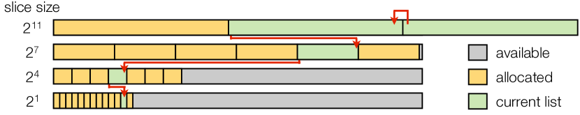
Figure 1: Organization of the active index segment where tweets are ingested. Increasingly larger slices are allocated in the pools to hold postings. Except for slices in pool 1 (the bottom pool), the first 32 bits are used for storing the pointer that links the slices together. Pool 4 (the top pool) can hold multiple slices for a term. The green rectangles illustrate the the “current” postings list that is being written into.

Our approach to address these issues is to create four separate “pools” for holding postings. Conceptually, each pool can be treated as an unbounded integer array. In practice, pools are large integer arrays allocated in $2^{15}$ element blocks; that is, if a pool fills up, another block is allocated, growing the pool. In each pool, we allocate “slices”, which hold individual postings belonging to a term. In each pool, the slice sizes are fixed: they are $2^{1}$, $2^{4}$, $2^{7}$, and $2^{11}$, respectively (see Figure 1). For convenience, we will refer to these as pools 1 through 4, respectively. When a term is first encountered, a $2^{1}$ integer slice is allocated in the first pool, which is sufficient to hold postings for the first two term occurrences. When the first slice runs out of space, another slice of $2^{4}$ integers is allocated in pool 2 to hold the next $2^{4}-1$ term occurrences (32 bits are used to serve as the “previous” pointer, discussed below). After running out of space, slices are allocated in pool 3 to store the next $2^{7}-1$ term occurrences and finally $2^{11}-1$ term occurrences in pool 4. Additional space is allocated in pool 4 in $2^{11}$ integer blocks as needed.

One advantage of this strategy is that no array copies are required as postings lists grow in length—which means that there is no garbage to collect. However, the tradeoff is that postings are non-contiguous and we need a mechanism to link the slices together. Addressing slice positions is accomplished using 32-bit pointers: 2 bits are used to address the pool, 19–29 bits are used to address the slice index, and 1–11 bits are used to address the offset within the slice. This creates a symmetry in that postings and addressing pointers both fit in a standard 32-bit integer. The dictionary maintains pointers to the current “tail” of the postings list using this addressing scheme (thereby marking where the next posting should be inserted and where query evaluation should begin). Pointers in the same format are used to “link” the slices in different pools together and, possibly, multiple slices in pool 4. In all but the first pool, the first 32 bits of each slice are used to store this “previous” pointer.

To conclude this section, we provide some performance figures, summarized from [2]. The basic configuration of an Earlybird server is a commodity machine with two quad-core processors and 72 GB memory. A fully-loaded active index segment with 16 million documents occupies about 6.7 GB memory. On such a segment, we achieve 17000 queries per second with a 95th percentile latency of $<$100 ms and 99th percentile latency of $<$200 ms using 8 searcher threads. In a stress test, we evaluated Earlybird indexing performance under near 100% CPU utilization. We achieve 7000 tweets per second (TPS) indexing rate at 95th percentile latency of 150 ms and 99th percentile latency of 180 ms. Indexing latency is relatively insensitive to tweet arrival rate; at 1000 TPS we observe roughly the same latencies as at 7000 TPS.

3.3 Generalizing the Solution

It is evident that Earlybird represents a specific instantiation of a general solution to the problem of dynamically allocating postings for real-time search: from a small number of large memory pools, we allocate increasingly larger slices for postings as more term occurrences are encountered. Within this general framework, a particular instantiation can be described by $Z=\langle z_{0},z_{1},...,z_{P-1}\rangle$, the slice size settings (as powers of two), where $P$ is the number of pools. For example, in the production deployment, $Z=\langle 1,4,7,11\rangle$. For best utilization of bits in addressing pointers, it is helpful to restrict $|P|$ to a power of two also.

Note that this framework provides a general solution to real-time indexing (not only tweets): we simply assume that slices hold spaces for postings and pointers to previous slices. In the case of tweets, both postings and pointers are 32-bit integers, but nothing in our model precludes other encodings. Thus, for the remainder of this paper, we measure postings in terms of “memory slots”. For simplicity, we assume that pointers also fit in a memory slot, but if this isn’t the case, a small constant factor adjustment will suffice.

How “optimal” is the current production deployment, compared to alternative configurations? Prior to this study, we have not attempted to answer this question in a rigorous, controlled fashion. In this paper, we tackle this question as follows: First, we define a cost model in terms of speed and memory usage, the two characteristics we seek to balance. Second, we develop an analytical model that allows us to assess the time and space costs of a particular configuration. Finally, for promising configurations identified by our analytical model, we follow up with experiments.

4 Data

Since our analytical model makes use of real data to estimate parameters, we begin by describing our datasets. For tweets, we used the Tweets2011 corpus created for the TREC 2011 microblog track. The corpus is comprised of approximately 16 million tweets over a period of two weeks (24th January 2011 until 8th February, inclusive) which covers both the time period of the Egyptian revolution and the US Superbowl. Different types of tweets are present, including replies and retweets. The corpus represents a sample of the entire tweet stream, but since tweets are hash partitioned across multiple Earlybird instances in production, experiments on these tweets is a reasonably accurate facsimile of studying an individual Earlybird instance. Even though we have access to all tweets, we purposely conducted experiments on this publicly available collection so that others will be able to replicate our results.

Three different sets of queries were used in our evaluation. First, we took the TREC 2005 terabyte track “efficiency” queries (50,000 queries total). Second, we sampled 100,000 queries randomly from the AOL query log [14], which contains around 10 million queries in total. Our sample preserves the original query length distribution. Finally, we used queries from the TREC 2011 microblog track. However, since there were only 50 queries (which is insufficient for efficiency experiments), we augmented the queries by first generating the power set of all query terms and then used the “related queries” API of a commercial search engine to harvest query variants. In this way, we were able to construct a set of approximately 3100 queries.

Our choice of these three datasets represented an attempt to balance several factors. Although we have access to actual Twitter query logs, experiments on them would have several drawbacks: First, due to their proprietary nature, our results would not be replicable. Second, the majority of Twitter queries are trending hashtags (or queries containing trending hashtags), which are not particularly interesting from an efficiency point of view (similar to head navigational queries in web search). Furthermore, we’d like to study the types of information needs that real-time search could solve, not exactly what the service is doing right now. Thus, triangulating based on three query sets paints a more complete picture: the AOL queries represent general web queries; the TREC efficiency queries are representative of ad hoc queries, closer to the “torso” of the query distribution (mostly informational, as opposed to navigational); finally, the TREC microblog queries represent a forward-looking conception of what real-time search might evolve into (at least according to retired intelligence analysts at NIST). Finally, all three of our datasets are available to researchers (we intend to release our expanded microblog queries).

5 Analytical Model

Given a collection of documents $\mathcal{C}$ and a set of queries $\mathcal{Q}$, we define a cost function for memory usage. The total memory “wasted” is equal to the memory allocated for postings minus the size of the postings list (i.e., number of postings), summed across all terms $t$ in the collection:

$$\sum_{t\in\mathcal{C}}{\left[\textrm{Memory}(t;Z)-\textrm{Size}(\textrm{Postings}(t))\right]}$$

Since the size of postings is constant for a given collection, we can simply define the memory cost as follows (which we’d like to minimize):

$$\mathcal{C}_{M}=\sum_{t\in\mathcal{C}}{\textrm{Memory}(t;Z)}$$ (1)

Similarly, let us define the time cost as the time it would take to read all postings (end to end) for all query terms in each query of $\mathcal{Q}$.

$$\mathcal{C}_{T}=\sum_{Q\in\mathcal{Q}}\sum_{q\in Q}{\textrm{TimeToRead}(\textrm{Postings}(q))}$$ (2)

Note that this cost function does not actually take into account time spent in query evaluation (e.g., intersection of postings lists for conjunctive query processing). We decided to factor out those costs for two reasons: First, to support a simpler model (since a large number of postings traversal techniques are available, each with different optimizations and tradeoffs). Second, even if we wished to, it is unclear how we could analytically model postings intersection time, which is a function of term occurrences in real-world data.

The advantage of our model is that instantiating it with parameters is fairly easy. If we assume that term frequencies in a collection follow a Zipfian distribution (a standard assumption in information retrieval), we can analytically estimate the memory cost for various $Z$ configurations. Similarly, if the postings length distribution of query terms is known, we can analytically model the time cost as well. With models of the two costs, we can find configurations that strike a desired memory/speed balance. The remainder of this section explains how we accomplish this.

5.1 Memory Cost Estimation

Given that the frequency of a term $t$ in a collection is $f_{r}$, and the pool settings is $Z=\langle z_{0},z_{1},...,z_{P-1}\rangle$, we can calculate the exact number of memory slots required to hold the postings list of term $t$. Let us define a step function $\mathcal{M}$ that maps a frequency to the number of memory slots required by configuration $Z$. First, we recursively define a set of thresholds $\theta_{i}$’s on the frequencies as follows:

$$\theta_{i}=\begin{cases}2^{z_{0}},&i=0\\ \theta_{i-1}+(2^{z_{i}}-1),&0<i\leq P\\ \theta_{P}+(i-P)\times(2^{z_{P-1}}-1),&i>P\\ \end{cases}$$

For each term frequency interval $\{f_{r}\in\mathbb{N}\,|\,\theta_{i-1}<f_{r}\leq\theta_{i}\}$ the value of the step function $\mathcal{M}$ can be computed as follows:

$$\mathcal{M}(f_{r})=\begin{cases}\theta_{0},&f_{r}\leq\theta_{0}\\ \theta_{i}+i,&\theta_{i-1}<f_{r}\leq\theta_{i}\;(i>0)\\ \end{cases}$$

This function computes the amount of memory (i.e., number of slots) that needs to be allocated to store pointers along with the actual postings. Given function $\mathcal{M}$, we can rewrite Equation (1) as:

$$\mathcal{C}_{M}=\sum\limits_{1\leq t\leq|V|}{\mathcal{M}(f_{r}(t))}$$ (3)

where $f_{r}(t)$ is the frequency of term $t$, and $|V|$ is the size of the vocabulary. Making a standard simplifying assumption, if we rank the terms in the collection with respect to their frequencies, the resulting pairs of $\langle r,\bar{f}_{r}\rangle$ (where $\bar{f}_{r}$ is normalized) form a Zipfian distribution, with the following probability mass function (PMF):

$$p(x)={x^{-\alpha}\over H_{|V|,\alpha}}$$ (4)

where $H_{\rho,\alpha}$ is the $\rho_{th}$ generalized harmonic number, and $\alpha$ is a parameter. From Equation (4), one can estimate a term frequency given the rank of term $r(t)$ and the total number of terms in the collection $N$ as:

$$f_{r}(t)=N\times p(r(t))$$

Thus, we can rewrite Equation (3) as follows:

$$\mathcal{C}_{M}=\sum\limits_{1\leq r\leq|V|}{\mathcal{M}(N\times p(r))}$$ (5)

where $r$ is the rank (with respect to frequency) of a term in the collection. Equation (5) gives an analytical model for estimating the memory cost of indexing a particular collection, given $N$ (total number of terms) and the characteristic Zipfian parameter $\alpha$.

Furthermore, we can speed up the computation of Equation (5) by exploiting the fact that the PMF of a Zipfian distribution is a one-to-one function. In this way, based on the definition of the step function $\mathcal{M}$, we have:

$$\theta_{i-1}<N\times p(r)\leq\theta_{i}\Rightarrow$$

$$\theta_{i-1}<{{N\times r^{-\alpha}}\over{H_{|V|,\alpha}}}\leq\theta_{i}\Rightarrow$$

$$\left(\theta_{i-1}\times{H_{|V|,\alpha}\over N}\right)<r^{-\alpha}\leq\left(\theta_{i}\times{H_{|V|,\alpha}\over N}\right)\Rightarrow$$

$${\theta_{i-1}^{-1\over\alpha}\times\underbrace{\left({H_{|V|,\alpha}\over N}\right)^{-1\over\alpha}}_{\text{$\beta$}}}>r\geq{\theta_{i}^{-1\over\alpha}\left({H_{|V|,\alpha}\over N}\right)^{-1\over\alpha}}\Rightarrow$$

$$\beta\theta_{i-1}^{-1\over\alpha}>r\geq\beta\theta_{i}^{-1\over\alpha}$$

Therefore, we can rewrite Equation (5) as follows by substituting the above in the definition of $\mathcal{M}$:

$$\mathcal{C}_{M} =\sum\limits_{1\leq r\leq|V|}{\mathcal{M}(N\times p(r))}$$

$$=\sum\limits_{|V|\geq r\geq{\beta\times\theta_{0}^{-1\over\alpha}}}{\theta_{0}}+\sum\limits_{\theta_{k}\neq\theta_{0}}{\sum\limits_{\beta\theta_{k-1}^{-1\over\alpha}<r\leq{\beta\theta_{k}^{-1\over\alpha}}}{(\theta_{k}+k)}}$$

$$=\left(|V|-\beta\theta_{0}^{-1\over\alpha}+1\right)\theta_{0}+\sum\limits_{\theta_{k}\neq\theta_{0}}{\beta\left(\theta_{k-1}^{-1\over\alpha}-\theta_{k}^{-1\over\alpha}\right)(\theta_{k}+k)}$$

To summarize, given a characteristic Zipfian parameter $\alpha$, the total number of terms $N$, and a configuration $Z$, we can compute the memory cost of indexing a particular collection in closed form.

5.2 Time Cost Estimation

We now turn to our analytical model of time cost, that of the sum of reading postings lists corresponding to all query terms. Let us assume that the cost of reading postings for a configuration $Z$ is equal to the sum of two components: (1) the cost of a sequential scan of equivalent postings lists stored as contiguous arrays and (2) the cost of following all pointers that link together non-contiguous slices between different pools. The first component is the same for all configurations (give a collection) so we can ignore as a constant. The number of pointers for a term $t$ with frequency $f_{r}$ can be computed easily given a particular configuration $Z$, so we can redefine our cost function as follows:

$$\mathcal{C}_{T}=\sum_{Q\in\mathcal{Q}}\sum_{q\in Q}{|\textrm{Pointers}(\textrm{Postings}(q);Z)|\times C_{p}}$$ (6)

where $C_{p}$ is the cost of following a pointer and $|\textrm{Pointers}(\cdot)|$ is the number of pointers needed in a particular postings list given a configuration $Z$. The number of pointers can be easily estimated given the step function $\mathcal{M}$ defined in Section 5.1. Thus, assuming we have an estimate of the distribution of $|\textrm{Pointers}(\cdot)|$ (from a query log), we are able to analytically compute a time cost.

What about $C_{p}$, the cost of following a particular pointer? Where exactly does this cost come from? Although all our index structures are held in main memory, latencies can still vary by orders of magnitude due to the design of cache hierarchies in modern processor architectures. Reading contiguous blocks of postings (in a slice) is a very fast operation since (1) neighboring postings are likely to be on the same cache line, and (2) predictable memory access when striding postings means that pre-fetching is likely to occur. On the other hand, when posting traversal reaches the end of a slice, the algorithm needs to follow the pointer to the next slice and begin reading there—most of the time, this will result in a cache miss, which will trigger a reference to main memory, which is significantly slower. Therefore, the cost $C_{p}$ is dominated by the cost of a cache miss. However, since we model $C_{p}$ as a constant, it is not necessary to estimate its actual value—therefore, our analytical time costs are modeled in abstract units of $C_{p}$.

To summarize, we can analytically estimate the time cost if we are given a hypothetical postings length distribution of query terms and the cost of a cache miss using Equation (6). We stress that this model is overly simplistic and does not account for time spent intersecting postings. Nevertheless, this simplification is acceptable since we use the analytical model only to guide our experiments on real data, and in our empirical results we do measure end-to-end query latency.

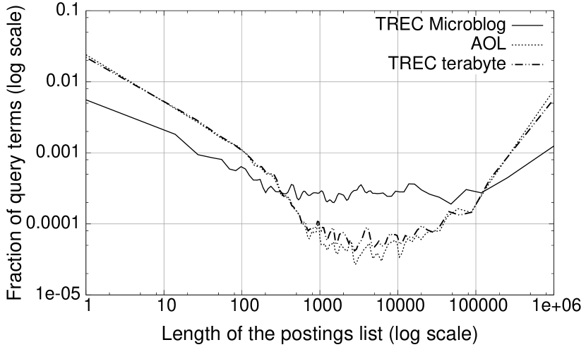
Figure 2: Postings length distribution for various query sets.

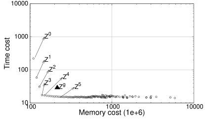
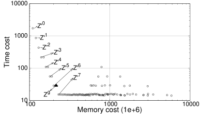
Figure 3: Scatter plot of analytical time cost $\mathcal{C}_{T}$ versus memory cost $\mathcal{C}_{M}$, where each point represents a configuration $Z$. In the right plot, the number of pools is restricted to 4, whereas in the left plot the number of pools can vary between 4 and 8. Scatter plots shown with same scale to facilitate comparison.

6 Analytical Results

Given a set of configurations $\mathcal{Z}=\{Z_{0},Z_{1},...,Z_{m}\}$, we can estimate the memory cost $\mathcal{C}_{M}$ as well as the simplified time cost $\mathcal{C}_{T}$ for any configuration $Z\subseteq\mathcal{Z}$. However, to complete our model we need to know the total number of terms $N$, size of the vocabulary $|V|$, and parameter $\alpha$. To determine these values, we divided the Tweets2011 collection into two equally-sized partitions and used the first half for parameter estimation; the second half is used in our actual experiments (described later). We determined $\alpha$ to be $1.0$, and $|V|$ and $N$ to $11\times 10^{6}$ and $76\times 10^{6}$ respectively.

As explained in Section 5.2, in order to estimate the time cost we need the distribution of length of postings for a set of query terms: this is shown for all three query sets in Figure 2. This figure shows that the overall distribution is similar among all query sets. In particular, the distribution from the AOL and terabyte queries are nearly identical. Data from the microblog queries give rise to a similarly shaped distribution, although with less emphasis at the extremes (both very common and very rare terms).

Given all these parameters, as well as the set of configurations $\mathcal{Z}$, we estimated the time cost and the memory cost for each configuration. On a scatter plot of the time versus memory cost, each configuration $Z\subseteq\mathcal{Z}$ would represent a point: points closer to the origin would be considered “better” configurations (faster, less memory).

Our strategy for exploring the configuration space was to first use our analytical model to quickly determine the tradeoffs associated with a large set of configurations, and then from those select a subset on which to run actual experiments. We considered slice sizes between 0 and 12 (inclusive) and pool sizes between 4 and 8 (inclusive) Another experiment specifically focused on four-pool configurations (as in the production system). Within these ranges, we computed the memory and time cost for all possible configurations. Since a scatter plot of all configurations would not be readable, we grouped the configurations into equally-sized buckets in terms of memory cost, and from each bucket, we picked the configuration that has the smallest time cost. Figure 3 shows the scatter plot constructed in this manner, using the AOL queries for the time cost estimates (results using other queries look nearly identical, and are not shown for space considerations). The right plot shows only four-pool configurations; the left plot shows all pool sizes between 4 and 8 (inclusive).

Based on these figures, we selected a set of candidate configurations that appear to present good time/cost tradeoffs. As our analytical models demonstrate, after a certain point the memory costs increase while the time costs level off, thereby making most of the configurations uninteresting. The more preferable configurations are those that appear near the origin in plots in Figure 3. The configurations selected for experimental analysis are noted.

7 Using Term History

There is one additional issue we consider. Given that Earlybird maintains several index segments in memory (one “active”, the rest read-only), it has easy access to historical term statistics from preceding index segments. It stands to reason that we can take advantage of this information. Although it seems obvious that such statistics would help, there are countervailing considerations as well. We have found that there is a great deal of “churn” in tweet content [11]; for example, approximately 7% of the top 10,000 terms (ordered by frequency) from one day are no longer in the top 10,000 on the next day. This makes sense since discussions on Twitter evolve quickly in response to breaking news events and idiosyncratic internet memes. Therefore, using term statistics may not actually help: a term that appeared frequently in the previous index segment may be related to a news story that is no longer “hot”, and as a result we might over-allocate memory and waste space.

To empirically determine how these factors play out on real data, we experimented with different policies for allocating the first slice (i.e., instead of always starting from the first pool, choose a pool with a larger slice size). We refer to this as the Starting Pool (SP) policy:

• SP($z_{0}$): This is the default policy that does not take advantage of any term frequency history. Every allocation starts from the first memory pool (i.e., $z_{0}$).

• SP($\lceil H(t)\rceil$): This policy starts indexing a term $t$ from the memory pool with the smallest slice size that is larger than the given historical frequency $H(t)$, i.e., from the previous index segment. That is, start from pool $p$ if $2^{z_{p-1}}<H(t)\leq 2^{z_{p}}$ or pool $P$ if $2^{z_{P-1}}\leq H(t)$.

• SP($\lfloor H(t)\rfloor$): According to this policy, indexing starts from the memory pool with the largest slice size that is smaller than the given historical frequency of a term $H(t)$. That is, start from pool $p$ if $2^{z_{p}}\leq H(t)<2^{z_{p+1}}$ or pool $P$ if $2^{z_{P-1}}\leq H(t)$.

• SP($\Lambda(H(t),z_{P-1})$): Based on this policy, if the frequency of a term $H(t)$ is greater than or equal to the slice size of the last pool (i.e., $2^{z_{P-1}}$), then indexing for that term starts from the last pool. Otherwise, indexing starts from the default pool, $z_{0}$. Function $\Lambda(H(t),z_{P-1})$ is $z_{P-1}$ if $H(t)\geq 2^{z_{P-1}}$ and $z_{0}$ otherwise. This basically divides postings into “long” and “short”, with the last slice size as the break point.

In all of the above policies, when we encounter an out-of-vocabulary term while indexing, we default to starting from the first memory pool (i.e., $z_{0}$).

Using the above schemes, we integrate history into our allocation policies. Therefore, our experiments explore not only the impact of different pool configurations, but also the role of history in improving cost.

8 Experimental Setup

To isolate only the effects that we are after, our experiments were not conducted on the codebase of the live production system, but rather a separate implementation, which was also implemented in Java. This allowed us to separate unrelated issues, such as management of multiple segments, query brokering, and synchronization of data structures from the core problem of memory allocation.

Experiments were performed on a server running Red Hat Linux, with dual Intel Xeon “Westmere” quad-core processors (E5620 2.4GHz) and 128GB RAM. This particular architecture has a 64KB L1 cache per core, split between data and instructions; a 256KB L2 cache per core; and a 12MB L3 cache shared by all cores of a single processor. However, all experiments were run on a single thread.

Our metrics were as follows: Evaluation of memory usage is quantified in terms of memory slots allocated once all tweets have been indexed (denoted $\mathcal{C}_{M}^{*}$). Similarly, time costs were measured with different queries after all the tweets have been indexed. This is a simplification, since in the production system query evaluation is interleaved with indexing. However, in production, concurrency is managed by an elaborate set of memory barriers, which is not germane to the current study. For our first time metric, we computed the per query average time to read postings for all query terms in their entirety, i.e.,

$$\mathcal{C}_{T}^{*}={1\over{|\mathcal{Q}|}}\sum_{Q\in\mathcal{Q}}\sum_{q\in Q}{\textrm{TimeToRead}(\textrm{Postings}(q))}$$

Unlike estimates from our analytical model $\mathcal{C}_{T}$, experimental costs are measured in milliseconds. In addition, we measured the per query average time to retrieve $k=100$ results in conjunctive query processing mode, i.e., the most recent 100 hits that contain all query terms (we denote this $\mathcal{R}_{100}$). We used a simple linear merge algorithm to perform postings intersection. Note that although more effective algorithms are available (e.g., SvS [5]), it remains an open question whether they are suitable for our type of index. Those techniques implicitly assume contiguous postings lists, since they use variants of binary search to seek through postings. We felt that to isolate the effects of different query evaluation algorithms, this was a reasonable choice.

So that we can evaluate the impact of different policies for taking advantage of term history, we divided the Tweets2011 corpus roughly in half (chronologically). All experiments were run on the second half, using statistic from the first half (where appropriate). Note that, somewhat coincidentally, half of the Tweets2011 corpus corresponds roughly to the size of the index segments deployed in production, adding realism to our results.

		postings traversal ($\mathcal{C}_{T}^{*}$)			top 100 retrieval ($\mathcal{R}_{100}$)
$Z$	$\mathcal{C}_{M}$	AOL	TB	MB	AOL	TB	MB
$Z^{g}=\langle 1,4,7,11\rangle$	90.2m	1.20 ($\pm$0.02)	0.86 ($\pm$0.08)	0.91 ($\pm$0.09)	2.31 ($\pm$0.01)	1.58 ($\pm$0.05)	1.39 ($\pm$0.02)
$Z^{0}=\langle 0,1,2,3,4,5,6,8\rangle$	15.9m	1.33 ($\pm$0.03)	0.93 ($\pm$0.07)	0.99 ($\pm$0.06)	2.02 ($\pm$0.05)	1.44 ($\pm$0.03)	1.57 ($\pm$0.02)
$Z^{1}=\langle 1,2,3,5,6,8,9,10\rangle$	29.1m	1.21 ($\pm$0.01)	0.76 ($\pm$0.12)	0.94 ($\pm$0.01)	1.90 ($\pm$0.08)	1.39 ($\pm$0.06)	1.50 ($\pm$0.03)
$Z^{2}=\langle 1,3,5,6,8,9,10,11\rangle$	34.9m	1.19 ($\pm$0.01)	0.74 ($\pm$0.03)	0.90 ($\pm$0.01)	1.89 ($\pm$0.01)	1.58 ($\pm$0.01)	1.39 ($\pm$0.02)
$Z^{3}=\langle 1,3,5,7,8,10,12\rangle$	45.1m	1.18 ($\pm$0.00)	0.74 ($\pm$0.02)	0.91 ($\pm$0.01)	2.30 ($\pm$0.03)	1.57 ($\pm$0.01)	1.69 ($\pm$0.01)
$Z^{4}=\langle 1,3,6,8,9,11,12\rangle$	49.8m	1.25 ($\pm$0.01)	0.74 ($\pm$0.01)	0.91 ($\pm$0.02)	2.30 ($\pm$0.01)	1.57 ($\pm$0.01)	1.70 ($\pm$0.01)
$Z^{5}=\langle 2,6,9,12\rangle$	112.1m	1.23 ($\pm$0.04)	0.90 ($\pm$0.07)	0.91 ($\pm$0.01)	2.30 ($\pm$0.04)	1.59 ($\pm$0.02)	1.69 ($\pm$0.03)
$Z^{\prime 0}=\langle 1,2,3,5\rangle$	19.7m	2.71 ($\pm$0.10)	1.75 ($\pm$0.04)	1.93 ($\pm$0.09)	3.14 ($\pm$0.28)	2.01 ($\pm$0.08)	2.15 ($\pm$0.14)
$Z^{\prime 1}=\langle 1,3,5,6\rangle$	24.0m	1.92 ($\pm$0.04)	1.20 ($\pm$0.03)	1.33 ($\pm$0.03)	2.42 ($\pm$0.13)	1.67 ($\pm$0.08)	1.76 ($\pm$0.03)
$Z^{\prime 2}=\langle 1,3,5,7\rangle$	27.6m	1.55 ($\pm$0.03)	1.12 ($\pm$0.17)	1.11 ($\pm$0.01)	2.20 ($\pm$0.07)	1.47 ($\pm$0.01)	1.69 ($\pm$0.05)
$Z^{\prime 3}=\langle 1,3,6,8\rangle$	37.3m	1.36 ($\pm$0.03)	1.00 ($\pm$0.01)	1.00 ($\pm$0.01)	2.04 ($\pm$0.03)	1.47 ($\pm$0.07)	1.62 ($\pm$0.10)
$Z^{\prime 4}=\langle 2,5,7,9\rangle$	59.6m	1.33 ($\pm$0.13)	0.89 ($\pm$0.07)	0.94 ($\pm$0.01)	1.94 ($\pm$0.01)	1.36 ($\pm$0.01)	1.57 ($\pm$0.01)
$Z^{\prime 5}=\langle 2,5,8,10\rangle$	71.9m	1.25 ($\pm$0.04)	0.83 ($\pm$0.07)	0.92 ($\pm$0.02)	1.91 ($\pm$0.02)	1.35 ($\pm$0.01)	1.58 ($\pm$0.05)
$Z^{\prime 6}=\langle 2,5,8,11\rangle$	86.4m	1.25 ($\pm$0.01)	0.91 ($\pm$0.02)	0.90 ($\pm$0.01)	2.34 ($\pm$0.03)	1.58 ($\pm$0.01)	1.38 ($\pm$0.02)
$Z^{\prime 7}=\langle 2,6,9,12\rangle$	112.1m	1.23 ($\pm$0.04)	0.90 ($\pm$0.07)	0.91 ($\pm$0.01)	2.30 ($\pm$0.04)	1.59 ($\pm$0.02)	1.69 ($\pm$0.03)

Table 1: Memory cost ($\mathcal{C}_{M}^{*}$), per query postings traversal time $\mathcal{C}_{T}^{*}$, and per query top k retrieval time ($\mathcal{R}_{k}$) for different pool configurations, using the AOL, terabyte (TB) and microblog (MB) queries on the Tweets2011 corpus (second half). Time is measured in ms, averaged across 3 trials, with 95% confidence intervals.

9 Experimental Results

9.1 Pool Configurations

Table 1 reports experimental results evaluating different pool configurations, showing memory cost ($\mathcal{C}_{M}^{*}$), per query postings traversal time $\mathcal{C}_{T}^{*}$, and per query top k document retrieval time ($\mathcal{R}_{k}$). In all cases, time is measured in milliseconds, and results are averaged across 3 trials, reported with 95% confidence intervals. We report results using the AOL, TREC terabyte (TB) and microblog (MB) queries in separate columns. The first row of the table shows our production configuration; the second “block” shows select configurations with the number of pools between 4 and 8 (inclusive); the third “block” restricts consideration to 4 pool configurations (as in production). In all cases we did not take term history into account, i.e., postings allocation began in the first pool, which corresponds to SP($z_{0}$).

When considering the 4 pool configurations, analytical modeling suggests that our production configuration $Z^{g}$ balances memory and time quite well (see Figure 3, right). This is indeed confirmed by our experimental results. Although during the original implementation of Earlybird no rigorous evaluations along these lines were conducted, the developers nevertheless honed in on a good point in the solution space. For example, $Z^{r4}$ and $Z^{r5}$ yield smaller footprints, and perhaps suggest faster query evaluation, but the results are inconclusive: no significant difference on $\mathcal{C}_{T}^{*}$; significantly better for two sets of queries on $\mathcal{R}_{100}$ but significantly worse for the third. Based on our results, it doesn’t appear possible to significantly speed up query evaluation, regardless of configuration. On the other hand, it is possible to dramatically decrease memory consumption by sacrificing speed, e.g., $Z^{r0}$ (as predicted by our analytical model).

Turning to configurations involving between 4 and 8 pools, we see opportunities to improve over the current production configuration. Configuration $Z^{2}$, for example, yields a substantially smaller memory footprint, while not slowing down query evaluation. However, the cost is more complex code to manage 4 versus 8 pools (of course, not modeled in our study). Nevertheless, these experiments point to possible future improvements in our production codebase.

Note that in this discussion, we avoided use of the term “optimal”, since that assumes a single objective metric for combining time and space in a sensical manner. Judgments on the relative merits of memory and speed must be made with respect to an organization’s resources, machine specifications, etc. For example, we can certainly imagine a case where $Z^{r0}$ is a good setting—e.g., for academic researchers, where resources are more constrained and latency demands are perhaps not as high. Therefore, throughout this paper, we have presented all results in terms of a memory/speed tradeoff. Any additional attempts to simplify would be not justified by real-world constraints.

Overall, we find that the predictions made by our analytical model ($\mathcal{C}_{M}$ and $\mathcal{C}_{T}$) match the empirical results quite reasonably ($\mathcal{C}_{M}^{*}$ and $\mathcal{C}_{T}^{*}$): not in terms of actual physical quantities, of course, but in terms of capturing the tradeoff between memory and speed. As we proceed from $Z^{0}$ to $Z^{5}$, and from $Z^{r0}$ to $Z^{r7}$, memory consumption increases while time trends downward. However, the overall time differences are not as large as Figure 3 would suggest (i.e., the vertical axes in the scatter plots are exaggerated). We note that time estimates produced by our analytical model are in terms of abstract $\mathcal{C}_{p}$ units (cost of referencing non-contiguous postings), not physical time. This congruence between analytical and experimental results justifies the assumptions made in our model, and validates the use of analytical estimates to quickly explore the large configuration space (which is too large to experimentally explore). On the other hand, the match between our analytical time cost $\mathcal{C}_{T}$ and top 100 retrieval time $\mathcal{R}_{100}$ is not as good—to be expected, since top $k$ retrieval involves postings intersection, which is difficult to model analytically. This points to the limitations of our approach and the need to perform experiments on real data.

			postings traversal ($\mathcal{C}_{T}^{*}$)			top 100 retrieval ($\mathcal{R}_{100}$)
$Z$	SP Policy	$\mathcal{C}_{M}^{*}$	AOL	TB	MB	AOL	TB	MB
$Z^{g}$	SP($z_{0}$)	90.2m	1.20 ($\pm$0.02)	0.86 ($\pm$0.08)	0.91 ($\pm$0.09)	2.31 ($\pm$0.01)	1.58 ($\pm$0.05)	1.39 ($\pm$0.02)
	SP($\lceil H(t)\rceil$)	104.5m	1.17 ($\pm$0.00)	0.74 ($\pm$0.00)	0.90 ($\pm$0.02)	2.23 ($\pm$0.01)	1.44 ($\pm$0.08)	1.39 ($\pm$0.01)
	SP($\lfloor H(t)\rfloor$)	94.8m	1.18 ($\pm$0.01)	0.76 ($\pm$0.01)	0.92 ($\pm$0.01)	2.23 ($\pm$0.02)	1.49 ($\pm$0.07)	1.39 ($\pm$0.01)
	SP($\Lambda(H(t),z_{P-1}$)	90.4m	1.17 ($\pm$0.00)	0.74 ($\pm$0.01)	0.91 ($\pm$0.01)	2.23 ($\pm$0.01)	1.49 ($\pm$0.06)	1.41 ($\pm$0.01)
$Z^{2}$	SP($z_{0}$)	34.9m	1.19 ($\pm$0.01)	0.74 ($\pm$0.03)	0.90 ($\pm$0.01)	1.89 ($\pm$0.01)	1.58 ($\pm$0.01)	1.39 ($\pm$0.02)
	SP($\lceil H(t)\rceil$)	40.8m	1.18 ($\pm$0.03)	0.74 ($\pm$0.02)	0.92 ($\pm$0.02)	2.26 ($\pm$0.04)	1.45 ($\pm$0.09)	1.39 ($\pm$0.01)
	SP($\lfloor H(t)\rfloor$)	43.2m	1.16 ($\pm$0.01)	0.73 ($\pm$0.00)	0.90 ($\pm$0.02)	2.26 ($\pm$0.04)	1.48 ($\pm$0.01)	1.39 ($\pm$0.01)
	SP($\Lambda(H(t),z_{P-1}$)	35.0m	1.17 ($\pm$0.01)	0.74 ($\pm$0.01)	0.91 ($\pm$0.02)	2.25 ($\pm$0.04)	1.50 ($\pm$0.02)	1.39 ($\pm$0.01)
$Z^{\prime 5}$	SP($z_{0}$)	71.9m	1.25 ($\pm$0.04)	0.83 ($\pm$0.07)	0.92 ($\pm$0.02)	1.91 ($\pm$0.02)	1.35 ($\pm$0.01)	1.58 ($\pm$0.05)
	SP($\lceil H(t)\rceil$)	77.7m	1.22 ($\pm$0.03)	0.75 ($\pm$0.01)	0.92 ($\pm$0.01)	1.90 ($\pm$0.01)	1.35 ($\pm$0.07)	1.51 ($\pm$0.02)
	SP($\lfloor H(t)\rfloor$)	73.9m	1.21 ($\pm$0.03)	0.77 ($\pm$0.02)	0.92 ($\pm$0.02)	1.90 ($\pm$0.01)	1.35 ($\pm$0.01)	1.50 ($\pm$0.02)
	SP($\Lambda(H(t),z_{P-1}$)	72.2m	1.20 ($\pm$0.00)	0.75 ($\pm$0.00)	0.92 ($\pm$0.01)	1.90 ($\pm$0.00)	1.35 ($\pm$0.01)	1.52 ($\pm$0.02)

Table 2: Effect of history-based Starting Pool policies. Results are organized the same manner as in Table 1.

9.2 Starting Pool Policies

In our second set of experiments, we investigated the impact of Starting Pool policies. As previously described, we divided the Tweets2011 corpus in half, gathered term statistics from the first half, and performed experiments on the second half. Experiments focused on particularly interesting pool configurations from the previous results: $Z^{2}\langle 1,3,5,6,8,9,10,11\rangle$, $Z^{\prime 5}\langle 2,5,8,10\rangle$, and the default production configuration, $Z^{g}\langle 1,4,7,11\rangle$.

When taking advantage of historical term statistics, there are many issues at play. First, we would expect faster query evaluation since the postings lists are more likely to be contiguous. This suggests less time overall when traversing all postings ($\mathcal{C}_{M}^{*}$), although the impact on $\mathcal{R}_{100}$ is unknown since top 100 retrieval is unlikely to require traversal of all postings. In terms of space, there are two considerations: starting at larger slices might save memory due to fewer pointers; on the other hand, if past statistics are not entirely predictive, memory will be wasted. How these factors balance out is an empirical question.

Table 2 shows results for various settings on our three sets of queries. Time is measured across 3 trials with 95% confidence intervals and the table is organized in a similar manner as Table 1. Note that SP($z_{0}$) is equivalent to using no term statistics, and is exactly the same as in Table 1 (row duplicated here for convenience).

Results show that in all cases different SP policies waste space (i.e, result in a larger memory footprint), without a clear convincing gain in speed. For example, the most aggressive policy SP($\lceil H(t)\rceil$) is the most wasteful (8–16% more memory). Despite the intuitive appeal of using historical term statistics, there does not seem to be a benefit, at least for the policies we studied.

10 Related Work

The problem of incremental indexing, of course, is not new. However, the literature generally explores different points in the design space. Previous work typically makes the assumption that the inverted lists (i.e., postings) are too large to fit in memory and therefore the index must reside on disk. Most algorithm operate by buffering documents and performing in-memory inversion (e.g., [8]), up to the capacity of a memory buffer. After the buffer is exhausted, inverted lists are flushed to disk; after repeated cycles of this process, we now face the challenge of how to integrate the in-memory portion of the index with one or more index segments that have been written to disk. There are three general strategies. The simplest is to rebuild the on-disk index in its entirely whenever the in-memory buffer is exhausted. This strategy is useful as a baseline, but highly inefficient in practice. The second option is to modify postings in-place on disk whenever possible [6, 16, 1], for example, by “eagerly” allocating empty space at the end of existing inverted lists for additional postings. However, no “pre-allocation” heuristic can perfectly predict postings that have yet to be encountered, so inevitably there is either not enough space or space is wasted. For the in-place strategy, if insufficient free space is available, to keep the postings contiguous, the indexer must relocate the entire inverted list elsewhere, requiring expensive disk seeks for copying the data. The third strategy avoids expensive random accesses by merging in-memory and portions of on-disk inverted lists whenever the memory buffer fills up [3, 10]: index merging takes advantage of the good bandwidth of disk reads and writes. In particular, Lester et al. [10] advocate a geometric partitioning and hierarchical merging strategy that limits the number of outstanding partitions, similar to [3].

One challenge of all three strategies described above is the handling of concurrent queries while in-memory and on-disk indexes are being processed. No matter what strategy, the operations will take a non-trivial amount of time, during which an operational system must continue serving queries efficiently. Many of the papers cited above do not discuss concurrent query evaluation. In contrast, this is an important aspect of our work in building a production system (although not specifically the focus of this paper).

In the buffer-and-flush approach, Margaritis and Anastasiadis [12] present an interesting alternative beyond the three strategies discussed above. They make a slightly different design choice: when the in-memory buffer reaches capacity, instead of flushing the entire in-memory index, they choose to flush only a portion of the term space (a contiguous range of terms based on lexicographic sort order), performing a merge with the corresponding on-disk portions of the inverted lists. The advantage of this is that it does not lead to a proliferation of index segments, compared to the work of Lester et al. [10].

Other than the obvious difference of in-memory vs. on-disk storage of the index, there is another more subtle point that distinguishes previous work from the Earlybird design. The approaches above generally try to keep postings lists contiguous—and for good reason, since disk seeks are expensive. There is, however, substantial cost in maintaining contiguity in terms of disk operations that are needed at index time. In contrast, since Earlybird index structures are in main memory, we found it acceptable for postings to be discontiguous. While it is true that traversing non-contiguous postings in memory results in cache misses, the cost of a cache miss is less in relative terms than a disk seek. Discontiguous inverted lists allow us to implement a zero-copy approach to indexing—once postings are written, we never need to copy them. In a managed memory environment such as the JVM, this leads to far less pressure on the garbage collector, since buffer copying yields garbage objects.

In another work, Lempel et al. [9] eschew inverted indexes completely and incrementally build document-centered representations, from which postings list are dynamically constructed and cached only in response to queries. The assumption is that more “heavyweight” index processes will run periodically (e.g., every 30 minutes), so that all other data structures can be considered transient. Although this design appears to be justified for the particular search environment explored (corporate intranet), these assumptions do not appear to be workable for our setting.

Another interesting point in the design space is represented by Google’s Percolator architecture [15], which is built on top of Bigtable [4]—a distributed, multi-dimensional sparse sorted map based log-structured merge trees. Percolator supports incremental data processing through observers, similar to database triggers, which provide cross-row transactions, whereas Bigtable only supports single-row transactions. This architecture represents a very different design from our system, which makes a fair comparison difficult. The performance figures reported by the authors suggest that Earlybird is much faster in indexing, but in fairness, this is an apples-to-oranges comparison. Percolator was designed to encompass the entire webpage ingestion pipeline, handling not only indexing but other aspects of document processing as well—whereas Earlybird is highly specialized for building in-memory inverted indexes.

Finally, a few notes about our strategy for allocating postings slices from fixed-size pools: there are some similarities we can point to in previous work, but some important differences as well. With the in-place update strategy where extra space for postings is pre-allocated, it is not much of a stretch to implement fixed block sizes that are powers of two. Brown et al. [1] allocate space for on-disk postings in sizes of 16, 32, 64, 128, $\ldots$ 8192. However, a few important differences (beyond in-memory vs. on-disk): Brown et al. copy postings each time a new block is allocated to preserve contiguity, whereas we don’t. In addition, the paper leaves open the method by which those blocks are allocated—whereas we describe a specific implementation based on fixed slice sizes in large pools (supporting efficient memory allocation, compact pointer addressing, etc.).

Tracing the lineage of various storage allocation mechanisms further back in time, we would arrive at a rich literature on general-purposes memory allocation for heap-based languages (e.g., malloc in C). According to the taxonomy of Wilson et al. [17], Earlybird’s allocation strategy would be an example of segregated free lists, an approach that dates back to the 1960s. Of course, since we’re allocating memory for the very specific purpose of storing postings, we can accomplish the task much more efficiently since there are much tighter constraints, e.g., no memory fragmentation, fixed sizes, etc. Nevertheless, it would be fair to think of our work as a highly-specialized variant of general purpose memory allocators for heap-based languages.

11 Future Work and Conclusion

Although the problem of online indexing is not new, we explore a part of the design space that makes fundamentally different assumptions compared to previous work: we consider index structures that are completely in memory and applications that have much tighter index latency requirements. There are many challenges for such applications, and we examined in depth one particular issue—dynamic postings allocation—within a general framework for incremental indexing. Our results are interesting in and of themselves, but we hope to achieve the broader goal of bringing real-time search problems to the attention of the research community. Hopefully, this will spur more work in this area.

12 Acknowledgments

This work has been supported in part by NSF under awards IIS-0916043, IIS-1144034, and IIS-1218043. Any opinions, findings, or conclusions are the authors’ and do not necessarily reflect those of the sponsor. The first author’s deepest gratitude goes to Katherine, for her invaluable encouragement and wholehearted support. The second author is grateful to Esther and Kiri for their loving support and dedicates this work to Joshua and Jacob.

References

- [1] E. Brown, J. Callan, and W. Croft. Fast incremental indexing for full-text information retrieval. VLDB, 1994.
- [2] M. Busch, K. Gade, B. Larson, P. Lok, S. Luckenbill, and J. Lin. Earlybird: Real-time search at Twitter. ICDE, 2012.
- [3] S. Büttcher and C. Clarke. Indexing time vs. query time trade-offs in dynamic information retrieval systems. CIKM, 2005.
- [4] F. Chang, J. Dean, S. Ghemawat, W. Hsieh, D. Wallach, M. Burrows, T. Chandra, A. Fikes, and R. Gruber. Bigtable: A distributed storage system for structured data. OSDI, 2006.
- [5] J. Culpepper and A. Moffat. Efficient set intersection for inverted indexing. ACM TOIS, 29(1):Article 1, 2010.
- [6] D. Cutting and J. Pedersen. Optimizations for dynamic inverted index maintenance. SIGIR, 1990.
- [7] J. Dean and S. Ghemawat. MapReduce: Simplified data processing on large clusters. OSDI, 2004.
- [8] S. Heinz and J. Zobel. Efficient single-pass index construction for text databases. JASIST, 54(8):713–728, 2003.
- [9] R. Lempel, Y. Mass, S. Ofek-Koifman, Y. Petruschka, D. Sheinwald, and R. Sivan. Just in time indexing for up to the second search. CIKM, 2007.
- [10] N. Lester, A. Moffat, and J. Zobel. Efficient online index construction for text databases. ACM TODS, 33(3), 2008.
- [11] J. Lin and G. Mishne. A study of “churn” in tweets and real-time search queries. ICWSM, 2012.
- [12] G. Margaritis and S. Anastasiadis. Low-cost management of inverted files for online full-text search. CIKM, 2009.
- [13] A. Moffat and J. Zobel. Self-indexing inverted files for fast text retrieval. ACM TOIS, 14(4):349–379, 1996.
- [14] G. Pass, A. Chowdhury, and C. Torgeson. A picture of search. InfoScale, 2006.
- [15] D. Peng and F. Dabek. Large-scale incremental processing using distributed transactions and notifications. OSDI, 2010.
- [16] A. Tomasic, H. Garcia-Molina, and K. Shoens. Incremental updates of inverted lists for text document retrieval. SIGMOD, 1994.
- [17] P. Wilson, M. Johnstone, M. Neely, and D. Boles. Dynamic storage allocation: A survey and critical review. International Workshop on Memory Management, 1995.
- [18] H. Yan, S. Ding, and T. Suel. Inverted index compression and query processing with optimized document ordering. WWW, 2009.
- [19] J. Zhang, X. Long, and T. Suel. Performance of compressed inverted list caching in search engines. WWW, 2008.