Measuring Agglomeration of Agglomerated Particles Pictures

Abstract.

In this article, we introduce a novel geometrical index $\delta_{\mathrm{agg}}$, which is associated with the Euler number and is obtained by an image processing procedure for a given digital picture of aggregated particles such that $\delta_{\mathrm{agg}}$ exhibits the degree of the agglomerations of the particles. In the previous work (Matsutani, Shimosako, Wang, Appl.Math.Modeling 37 (2013), 4007-4022), we proposed an algorithm to construct a picture of agglomerated particles as a Monte-Carlo simulation whose agglomeration degree is controlled by $\gamma_{\mathrm{agg}}\in(0,1)$. By applying the image processing procedure to the pictures of the agglomeration particles constructed following the algorithm, we show that $\delta_{\mathrm{agg}}$ statistically reproduces the agglomeration parameter $\gamma_{\mathrm{agg}}$. agglomeration, digital image processing procedure, Euler number

1. Introduction

Nano-composite materials have a promising future from industrial viewpoints, since in the materials, geometrical properties in micro-scale play crucial roles and generate novel and various macro-material properties. By controlling the geometrical properties or shapes, we can design the macro-material properties drastically. Following Kelvin’s philosophy of science [6], it is quite important to evaluate such geometrical properties or shapes if one needs to control them using the scientific knowledge.

On the other hand, the smaller the particle is, the larger the effect of the surface energy is. It means that small particles are apt to aggregate or agglomerate in general because the agglomeration and the aggregation of the particles decrease the total surface energy and contribute to the stability of the system. When we handle materials consisting of nano-particles, the agglomeration and the aggregation are ones of the most important shapes since they sometimes have an effect on the generations of the macro-materials properties. In this article, we focus on them. It is said that the aggregation is due to chemical effects whereas the agglomeration comes from physical effects. Since in a computational model, there is no difference between them, we call both agglomeration in this article, though in spatial point analysis [7], the aggregation is chosen in general.

In the article [11], in order to find the agglomeration effect in the electric conductivity of the nano-composite material, we study the electric conductivity in an agglomerated continuum percolation model and show that the agglomeration of particles affects the macro-material properties. The purpose of this article is to evaluate the agglomeration in the binary digital images of agglomerated particles, e.g., of electron-microscopes.

For the same purpose, so many evaluation methods and definitions of the agglomeration are proposed to evaluate the agglomeration. In spatial point analysis, the distribution of the nearest distance particles, Clark-Evans index and so on are considered [2, 7]. Further Miles considered the problem in [12] and showed the two-dimensional overlapping ratio of the random configurations in three dimensional space. These investigations on the agglomeration have been done in the framework of the statistical analysis for a point pattern $\mathcal{R}=\{p_{i}\in{\mathbb{R}}^{2}\}$ which are given as statistical configurations of (finite) points. In the analysis, $\mathcal{R}_{r}:=\overline{\bigcup_{p\in\mathcal{R}}U_{r,p}}$ is investigated, which is a configuration of disks whose centers are $\mathcal{R}$, where $U_{\varepsilon,p}:=\{q\in{\mathbb{R}}^{2}\ |\ |q-p|<\varepsilon\ \}$. The Euler number, the area and the perimeter of $\mathcal{R}_{r}$ for several point processes $\mathcal{R}$’s are computed as morphological indices or the Minkowski characterization [7]. When $\mathcal{R}$ is given by the point process of the Poisson type, Stoyan, Kendall and Mecke studied their behaviors based on the study of Miles [12] and found that

(1) $$e(x)=(1-x)\mathrm{e}^{-x},\quad a(x)=\frac{1}{x}(1-\mathrm{e}^{-x}),\quad\ell(x)=\mathrm{e}^{-x},\quad$$

where $e(x)$, $a(x)$, and $\ell(x)$ are the normalized versions of the Euler number, the area and the perimeter of $\mathcal{R}_{r}$, and $x$ is a normalized radius $r$ [15, 9]. Mecke and Stoyan studied the difference among point patterns given by different processes in terms of these behaviors [9]. Further Tscheschel and Stoyan also studied the statistical reconstruction of random point patterns [16].

However in the nano-composite materials consisting of nano-particles, the particles themselves sometimes have complicated shapes, such as ellipsoids and rods, as we investigated in [10]. In other words, the configuration is not given by a point pattern with radius $r$ in general and further its parts are overlapped like (d) in Figures 2 and 3. Hence it is basically an ill-posed problem to define the center points of actual agglomerated particles in a given picture, e.g., of an electron-microscopes.

Thus it is natural to consider geometrical properties of the binary picture as a general geometrical object embedded in ${\mathbb{R}}^{2}$.

Recently MacPherson and Schweinhart proposed a novel method which evaluates the complicatedness of the complicated geometric objects embedded in a plane ${\mathbb{R}}^{2}$ in terms of the persistent homology [8]. The persistent homology gives the homological quantities of the persistent modules with real parameter [3, 17]. It could be regarded as a generalization of homotopical approach in traditional algebraic topology [1], though the deformation does not preserve homotopical properties. For a geometrical object $\mathcal{M}\subset{\mathbb{R}}^{2}$, we consider a family of objects with a real parameter $t\in[0,1]$, i.e., $\{\mathcal{M}_{t}\ |t\in[0,1]\}$.

By considering union of the $\varepsilon$-neighborhood of each point in $\mathcal{M}$, $\mathcal{M}_{\varepsilon}:=\overline{\bigcup_{p\in\mathcal{M}}U_{\varepsilon,p}}$, induced from the standard Euclidean topology, MacPherson and Schweinhart evaluated the complexity of the geometrical objects. The persistent homology shows the distributions of topological changes generated by the persistent modules (vector spaces) induced from $\mathcal{M}_{t^{\prime}}\subset\mathcal{M}_{t}$ for $t^{\prime}<t$.

As in [8], to investigate the effect from the standard topology of Euclidean space and to evaluate the complexity, we use the one-parameter family of a deformed geometrical object, and propose a digital image processing procedure which characterizes the shapes in pictures of the electric microscope in this article. (In Section 3, we give the list of assumed geometrical features of the pictures which we deal with.) For an appropriate geometrical object $\mathcal{M}$ in ${\mathbb{R}}^{2}$ with a characteristic lengths $\ell_{1}$ and $\ell_{2}$, we also handle the family of geometrical objects $\{\mathcal{M}_{t}=\overline{\bigcup_{p\in\mathcal{M}}U_{t,p}}\$ $|t\in[\ell_{1},\ell_{2}]\}$. We define the cumulus of the absolute differential Euler number (CADE) by,

(2) $${\mathcal{E}}(\mathcal{M};\ell_{2},\ell_{1}):=\int_{\ell_{1}}^{\ell_{2}}\left|\frac{d\chi(\mathcal{M}_{t})}{dt}\right|dt,$$

where $\chi(X)$ is the Euler number of $X$. ${\mathcal{E}}(\mathcal{M};\ell_{2},\ell_{1})$ evaluates how many topology changes occur for the deformation $[\ell_{1},\ell_{2}]$.

As we are concerned with the image processing procedure for images of the electron-microscopes, we will customize ${\mathcal{E}}(\mathcal{M};\ell_{2},\ell_{1})$ as ${\hat{\mathcal{E}}}(\mathcal{M};\ell_{2},\ell_{1})$ for any binary pictures as an image processing procedure, which is shown in Section 3 more precisely. Further in the nano-materials, there are several scales and one of them is the size of the particles and the resolution of the digital picture is given by the pixel size. We fix $\ell_{1}$ and $\ell_{2}$ by the pixel size and the (average) radius $\rho$ of the particle respectively to evaluate the agglomeration and propose an agglomeration index,

(3) $$\delta_{\mathrm{agg}}(\mathcal{M}):=\frac{\alpha}{{\hat{\mathcal{E}}}_{p(\mathcal{M})}}({\hat{\mathcal{E}}}_{p(\mathcal{M})}-{\hat{\mathcal{E}}}(\mathcal{M};\rho,a)),$$

where $p(\mathcal{M})$ is the volume fraction of $\mathcal{M}$ in the region $\mathcal{W}$ $(\mathcal{M}\subset\mathcal{W}\subset{\mathbb{R}}^{2})$, ${\hat{\mathcal{E}}}_{p}$ is the average of a “standard pattern of volume fraction $p$” as mentioned in Section 3, and $\alpha$ is a normalized factor $1.2$.

In order to estimate our agglomeration parameter $\delta_{\mathrm{agg}}$, we performed Monte-Carlo simulations for the binary agglomeration configurations of particles whose degree of the agglomeration is parameterized by $\gamma_{\mathrm{agg}}$, since in the article [11], we proposed a statistical model which numerically generates the agglomeration of particles controlled by the parameter $\gamma_{\mathrm{agg}}$ in order to investigate the properties of the agglomerated continuum percolation models. In Section 2, we review the algorithm following the article [11]. For a given parameter $\gamma_{\mathrm{agg}}\in[0,1]$, we can statistically construct the infinitely many configurations with the same level of the agglomerations. As the continuum percolation model is the same as a germ-grain model in the study for the point process [7], there are several other algorithms to construct aggregational germ-grain models, such as Neyman-Scott processes [7], though they are different from ours; ours is for the actual pictures of electron-microscopes of the agglomerated nano-composite materials with the radius $\rho$ as mentioned in [11]. We apply the index $\delta_{\mathrm{agg}}$ to evaluate the agglomeration of the agglomerated configuration which is generated by the forward method in [11]. Then the relevancy between $\delta_{\mathrm{agg}}$ and $\gamma_{\mathrm{agg}}$ is shown in Section 4, i.e., in Figure 7 and Table 3. We also mention the relation between our $\delta_{\mathrm{agg}}$ and the well-established Clark-Evans index in Section 4.

2. Agglomerate configuration

In order to explain what is the agglomeration that we are concerned with, we show the agglomeration configurations in computer science, which we handled in [11]. In the article [11], we proposed a construction of the agglomerated continuum percolation models which apparently recover geometric properties of real nano-particles, though there are several other agglomerated percolation models such as Neyman-Scott processes [7, 15, 16]. Since our method has a single parameter $\gamma_{\mathrm{agg}}$ besides a typical length $\rho$ whereas others are given as point processes with several parameters, we believe that ours is a natural model for the actual pictures of electron-microscopes of the agglomerated nano-composite materials with the radius $\rho$. As shown in Figures 2 and 3, we have the agglomerated configuration of particles depending upon a agglomeration parameter $\gamma_{\mathrm{agg}}\in[0,1]$. In this section, we show the geometrical setting of agglomerated continuum percolation model in [11], which is modeled by the agglomerated clusters in nature.

We set particles parameterized by their center positions $(x,y)$ into a box-region $\mathcal{W}:=[0,L]\times[0,L]$ at random and get a configuration $\mathcal{M}_{n}$ as a model of continuum percolation. The particle corresponds to a disk with the same radius $\rho$, $B_{x_{i},y_{i}}:=\{(x,y)\in\mathcal{W}\ |\ |(x,y)-(x_{i},y_{i})|\leq\rho\}$. The configuration $\mathcal{M}_{n}$ is given by $\mathcal{M}_{n}:=\bigcup_{i=1}^{n}B_{x_{i},y_{i}}$.

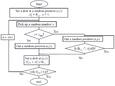
Figure 1. The flowchart of the algorithm which constructs the agglomerated configurations.

The flowchart in Figure 1 illustrates the algorithm. As the initial state, the configuration $\mathcal{M}_{0}$ has no particle. As the first step, for a uniform random position $(x,y)\in\mathcal{W}$, we set a particle $B_{x,y}$ whose center is $(x,y)$ and the radius is $\rho$, i.e., $\mathcal{M}_{1}:=B_{x,y}$.

For the $(n+1)$-th step, we take a position $(x,y)$ at uniform random in $\mathcal{W}$, and another random parameter $\gamma$ at uniform random in $[0,1]$. If $\gamma$ is greater than $\gamma_{\mathrm{agg}}$, we set $\mathcal{M}_{n+1}:=\mathcal{M}_{n}\bigcup B_{x,y}$. We now allow the particles to overlap each other.

For the case $\gamma\leq\gamma_{\mathrm{agg}}$, we first check whether the disk $B_{x,y}$ is connected with the previous configuration $\mathcal{M}_{n}$ or not. For the case $\mathcal{M}_{n}\bigcap B_{x,y}\neq\emptyset$, we employ the position and set $\mathcal{M}_{n+1}:=\mathcal{M}_{n}\bigcup B_{x,y}$. Otherwise or $\mathcal{M}_{n}\bigcap B_{x,y}=\emptyset$, we abandon the position and go on to take another uniformly random position $(x,y)$ in $\mathcal{W}$ until we find the position which supplies a connected particle $B_{x,y}$ with $\mathcal{M}_{n}$.

In other words, for the case $\gamma\leq\gamma_{\mathrm{agg}}$, the added particle must be connected with the previous configuration $\mathcal{M}_{n}$. Thus, $\gamma_{\mathrm{agg}}$ stands for the agglomeration of the particle system.

By monitoring the total volume fraction which is a function of $\mathcal{M}_{n}$ and is denoted by ${p}(\mathcal{M}_{n})$, we go on to put the particles as long as ${p}(\mathcal{M}_{n})\leq p$ for a given volume fraction $p$. We find the step $n(p)$ such that ${p}(\mathcal{M}_{n(p)-1})\leq p$ and ${p}(\mathcal{M}_{n(p)})>p$. Since we assume that the difference between ${p}(\mathcal{M}_{n(p)-1})$ and ${p}(\mathcal{M}_{n(p)})$ is sufficiently small, we regard ${p}(\mathcal{M}_{n(p)})$ as the volume fraction $p$ itself hereafter under this accuracy.

Since in the Monte-Carlo method, we use the pseudo-randomness to simulate the random configuration $\mathcal{M}_{n(p)}$ for given $p$ and $\gamma_{\mathrm{agg}}$, the configuration $\mathcal{M}_{n(p)}$ depends upon the seed $i_{S}$ of the pseudo-randomness which we choose. We let it be denoted by $\mathcal{M}_{\gamma_{\mathrm{agg}},p,i_{S}}$ or its statistical quantity by $\mathcal{M}_{\gamma_{\mathrm{agg}},p}$.

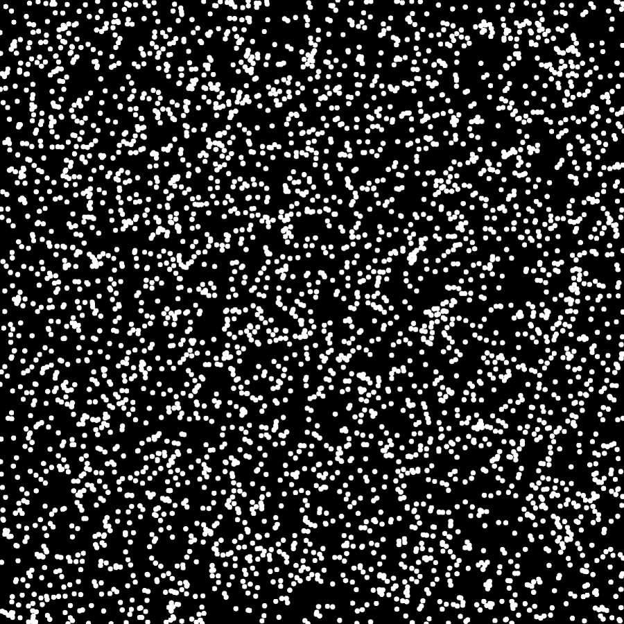
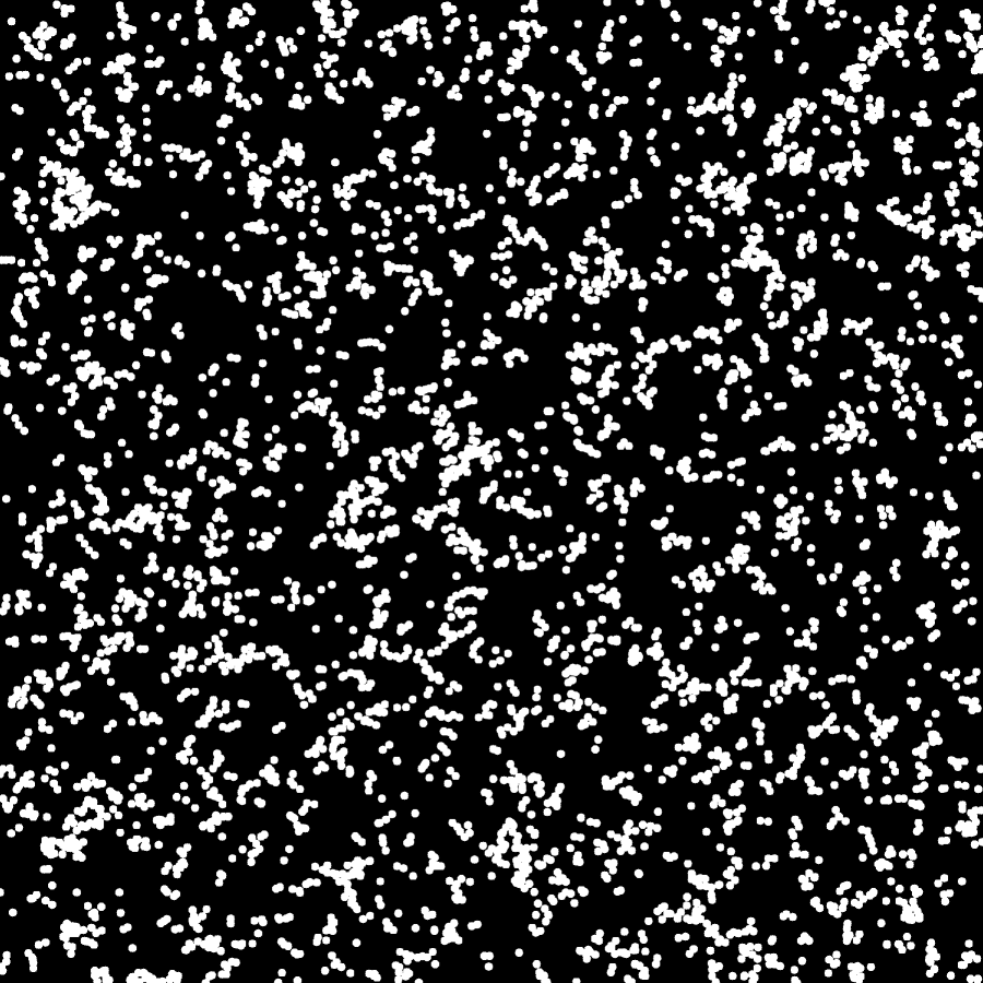
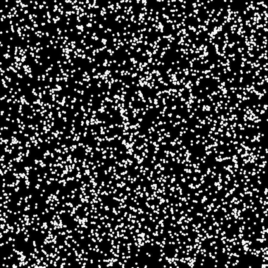
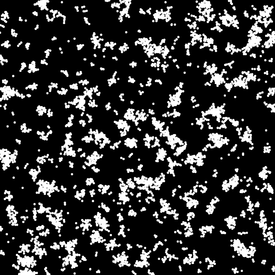
(a) (c) (b) (d)

Figure 2. The agglomerated configurations of $p=0.2$: These (a), (b), (c), and (d) show the configurations with the agglomeration parameter $\gamma_{\mathrm{agg}}$ $=0.0,0.3,0.6$ and $0.9$ respectively.

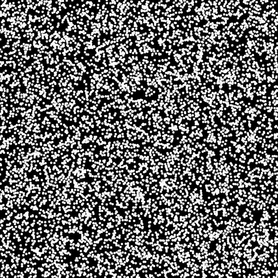
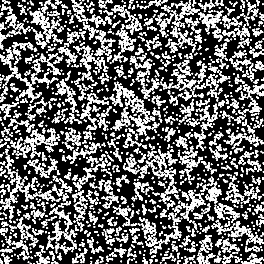
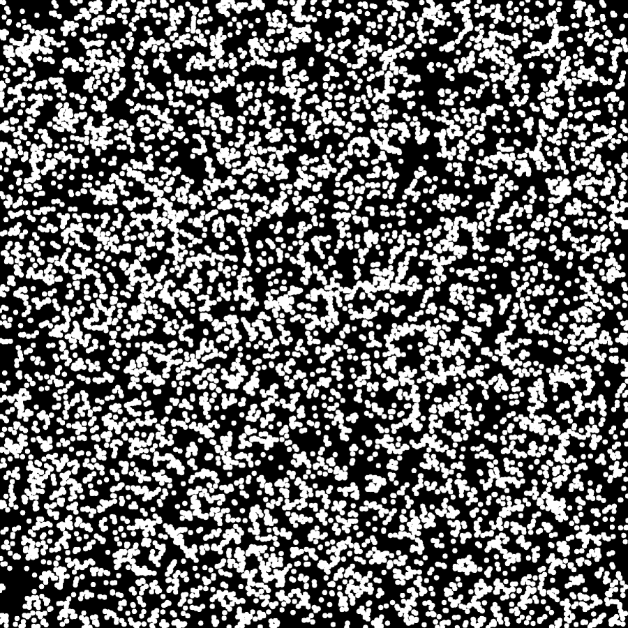
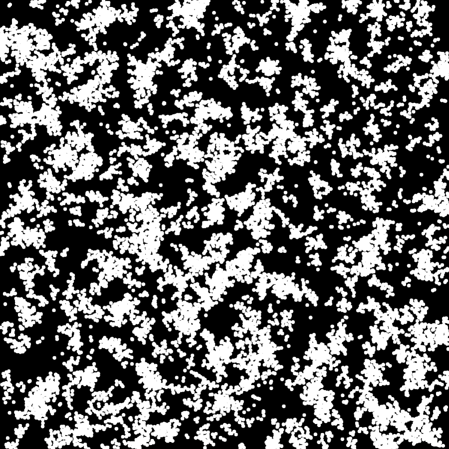
(a) (c) (b) (d)

Figure 3. The agglomerated configurations of $p=0.4$: These (a), (b), (c), and (d) show the configurations with the agglomeration parameter $\gamma_{\mathrm{agg}}$ $=0.0,0.3,0.6$ and $0.9$ respectively.

For sufficiently large $L$ and $L^{\prime}$ ($\rho\ll L^{\prime}<L$) and for a window $\mathcal{W}_{(x,y)}^{\prime}:=[x,x+L^{\prime}]\times[y,y+L^{\prime}]\subset\mathcal{W}$, the volume fraction $p^{\prime}(x,y)$ in $\mathcal{W}_{(x,y)}^{\prime}$ is proportional to the number of particles $N^{\prime}(x,y)$ in $\mathcal{W}_{(x,y)}^{\prime}$, i.e., there is a constant number $\lambda$ such that $p^{\prime}(x,y)=\lambda N^{\prime}(x,y)$. Further $\mathcal{M}_{\gamma_{\mathrm{agg}},p,i_{S}}$ is isotropic and independently scattered and thus the asymptotic behavior of $\mathcal{M}_{\gamma_{\mathrm{agg}},p,i_{S}}$ is a kind of Poisson process [7, p.66] though we have the condition $L^{\prime}\gg\rho$.

Further though our algorithm for $\gamma_{\mathrm{agg}}>0$ is not Markov process because each step depends on the previous configuration, we should note that it preserves a hierarchical structure for fixed $i_{S}$ and $p>p^{\prime}$,

$$\mathcal{M}_{\gamma_{\mathrm{agg}},p^{\prime},i_{S}}\subset\mathcal{M}_{\gamma_{\mathrm{agg}},p,i_{S}}.$$

As we will show the assumed geometric properties of pictures in Section 3, the pictures which we will deal with are illustrated in Figures 2 and 3, which are obtained following our algorithm. Our more concrete aim of this article is to recover the parameter $\gamma_{\mathrm{agg}}$ for a given configuration $\mathcal{M}_{\gamma_{\mathrm{agg}},p}$ in a statistical meaning. More precisely, our study is to find statistical monotone functions of $\gamma_{\mathrm{agg}}$ and to show that one of them is $\delta_{\mathrm{agg}}$ in (3).

3. Evaluation of Agglomeration for a configuration $\mathcal{M}_{p,\gamma_{\mathrm{agg}}}\subset\mathcal{W}$

As we are concerned with the evaluation method as a digital image processing procedure [13], in this section, we illustrate our algorithm for a picture which only has binary values. It is natural that we assume the configuration $\mathcal{M}$ (implicitly $\mathcal{M}_{p,\gamma_{\mathrm{agg}},i_{S}}$ and a picture of nano-composite material in an electron-microscope) has the following structures:

1. $L$ is sufficiently larger than $\rho$ so that the particles of $\mathcal{M}$ are a representative of sufficiently randomized configurations; we could assume the Euclidean invariance (translation, rotation and inversion) statistically; after averaging them, the physical and geometrical quantities are invariant for any Euclidean action $\mathrm{E}(2)$ up to the statistical deviation. If the deviation is not small, we could consider the series of $\{\mathcal{M}_{p,\gamma_{\mathrm{agg}},i_{S}}\ |\ i_{S}\}$. (It means that for the case of the pictures of the electron-microscopes, we could assume that the researchers prepare the series of pictures of a material or materials which are produced in the same conditions.)

2. It is assumed that the volume fraction is less than the percolation threshold of two dimensional continuum percolation models. (For the case of nano-composite material which is based upon the percolation theory, the volume fraction around the percolation threshold $0.2\sim 0.3$ in three dimensional percolation models is concerned, which is far less than the percolation threshold of two dimensional case $0.5\sim 0.7$.)

3. There are three sizes of the system or the picture $\mathcal{M}_{p,\gamma_{\mathrm{agg}}}$ (and the digital image of nano-composite material of an electron-microscope);

   1. the (average) size of particles, which is given by $\rho$,

   2. the analyzed size of the system, which is, now, given by $L$ as mentioned above, and

   3. the pixel size $a$, which is also controlled so that we can discriminate the particles in concerned resolution.

Under these assumptions, we consider geometry of $\mathcal{M}$. It is known that the $\varepsilon$-neighborhood, $\mathcal{M}_{\varepsilon}=\overline{\bigcup_{p\in\mathcal{M}}U_{\varepsilon,p}}\bigcap\mathcal{W}$, can be realized by the so-called level set method in computer science [14]. Let $d:\mathcal{W}\to{\mathbb{R}}$ be the signed distance from the boundary $\partial\mathcal{M}$ so that the outer side is assigned to the positive distance and the inner side is to the negative one, and then the geometrical object in the level set method can be regarded as $\mathcal{L}_{t}=d^{-1}(t)$. $\mathcal{M}_{t}$ of $(t>0)$ is equal to $d^{-1}([0,t])\bigcup\mathcal{M}$ and $\mathcal{L}_{t}=\partial\mathcal{M}_{t}$. For $t<0$ case, $\mathcal{L}_{t}=\partial(\overline{\bigcup_{p\in\partial\mathcal{M}}U_{t,p}})\setminus\mathcal{L}_{-t}$. Hence by means of the level set method, we can compute the more precise geometrical properties beyond the pixel size resolution even on the image defined over a subset of ${\mathbb{Z}}^{2}$.

However in the digital image processing procedure, we investigate the geometrical object up to the pixel size resolution in general. Further we must pay our attentions on the computational cost if we apply our method to real problems in industry, though level set function method requires higher computational cost than a simple digital image processing procedure. Hence in this article, we use the thickening scheme in the image processing procedure [13] instead of the level set function. Though the ordinary thickening scheme has anisotropic behavior, it does not have a serious effect on the result because the configuration itself is isotopic or rotational invariant. We use the modified thickening scheme, which improves the anisotropic behavior shown in Section 4. Let $\mathcal{M}^{(i)}$ be the $i$-th thickening of $\mathcal{M}$ in $\mathcal{W}$. We modify the CADE (2) as an image processing procedure by

$${\hat{\mathcal{E}}}(\mathcal{M};n_{2}a;n_{1}a):=\sum_{i=n_{1}+1}^{n_{2}}|\chi(\mathcal{M}^{(i)})-\chi(\mathcal{M}^{(i-1)})|.$$

In the persistent homology, the Betti number is handled in general. Since the computational cost to the evaluation of the Euler number is not so high and the Euler number could be compared with the results in [7, 15], we consider the behavior of the Euler numbers of $\mathcal{M}_{t}$ in this article. More precisely though there is no guarantee that $\chi(\mathcal{M}_{t})$ is equal to $\chi(\mathcal{M}^{(i-1)})$ for $t\in[a(i-1/2),a(i+1/2))$, we handle $\chi(\mathcal{M}^{(i-1)})$; as mentioned above, in digital analysis, we should basically neglect finer geometrical difference than the pixel size resolution and we follow the principle. In the complicated system, we believe that it is quite important how many topology changes occur for the $i$-step, and the difference of the Euler number can represent the behavior.

Further the agglomeration can be discriminated whether the particles are connected or not. From (1), if $L/\rho$ is sufficiently large, even for $\gamma_{\mathrm{agg}}=0$ and small $p$, ${\hat{\mathcal{E}}}(\mathcal{M}_{0,p},na,0)$ does not vanish $n>0$, in general, due to the randomness of the configurations. Further the behavior ${\hat{\mathcal{E}}}(\mathcal{M};n_{1}a,n_{2}a)$ of $n_{1},n_{2}\in[0,\rho/a)$ is quite important since the agglomeration suppresses the topology change in the interval as illustrated in Figures 4 and 5.

Due to the randomness of the configurations and the agglomeration, it is not so important whether the Euler numbers increase or decrease, but the topological change for the deformation is quite important. We define the agglomeration parameter $\delta^{(n_{1},n_{2})}_{agg}$ in (3) more precisely

(4) $$\delta^{(n_{2},n_{1})}_{\mathrm{agg}}(\mathcal{M})=\frac{\alpha}{{\hat{\mathcal{E}}}^{(n_{2},n_{1})}_{p(\mathcal{M})}}({\hat{\mathcal{E}}}^{(n_{2},n_{1})}_{p(\mathcal{M})}-{\hat{\mathcal{E}}}(\mathcal{M};n_{2}a,n_{1}a)),$$

where $p(\mathcal{M})$ is the volume fraction of $\mathcal{M}$, ${\hat{\mathcal{E}}}^{(n_{2},n_{1})}_{p}$ is the average of the standard patterns of volume fraction $p$, and $\alpha$ is a normalized factor $1.2$, which is chosen as a result of the comparison with $\gamma_{\mathrm{agg}}$ (see Table 3). The standard pattern means the pattern of $\gamma_{\mathrm{agg}}=0$ with the same radius in the same window $\mathcal{W}$. Then $\delta^{(n_{2},n_{1})}_{{\mathrm{agg}}}(\mathcal{M}_{\gamma_{\mathrm{agg}},p})$ characterizes how many topological changes occur in the interval $(n_{1}a,n_{2}a)$ for the deformations for each particle in $\mathcal{M}_{\gamma_{\mathrm{agg}},p}$ by normalized by ${\hat{\mathcal{E}}}^{(n_{2},n_{1})}_{p}$.

4. Numerical Computation and Results

Let us show the relevance between $\delta_{p}$ and $\gamma_{p}$ by the Monte-Carlo simulations following the algorithm mentioned in Section 2. Using the algorithm in Section 2, we have ten pictures of agglomerated particles for each $\gamma_{\mathrm{agg}}=0,0.3,0.6$ and $0.9$, and for each $p=0.1,0.2,0.3$ and $0.4$ by letting $L=2400$ and $\rho=10$ as in Figures 2 and 3.

On the thickening to compute the CADE, we use two types thickening process,

$$\begin{array}[]{rl}\mbox{type I: }&\ \Box\ \to\ \begin{matrix}&\Box&\\ \Box&\Box&\Box\\ &\Box&\\ \end{matrix},\\ \mbox{type II: }&\ \Box\ \to\ \begin{matrix}\Box&\Box&\Box\\ \Box&\Box&\Box\\ \Box&\Box&\Box\\ \end{matrix},\\ \end{array}$$

such that we generate an octagon asymptotically and approximates the area of the disks;

Table 1. The pattern of thickening

steps	type	radius	area	n.of pixels
1	II	0.5	0.785	1
2	I	1.5	7.065	9
3	I	2.5	19.625	21
4	I	3.5	38.465	37
5	II	4.5	63.585	69
6	I	5.5	94.985	97
7	I	6.5	132.665	129
8	II	7.5	176.625	185
9	I	8.5	226.865	229
10	I	9.5	283.385	277

In other words, on the thickening process, we use the deformation in digital process procedure for each point which is given in Table 1. Further for each point, we consider the thickening:

$$\begin{array}[]{cccccccccccccccccccccc}&&&&&&0&0&0&0&0&0&0&&&&&&\\ &&&&&0&9&9&9&9&9&9&9&0&&&&&\\ &&&&0&9&8&8&8&8&8&8&8&9&0&&&&\\ &&&0&9&8&8&7&7&7&7&7&8&8&9&0&&&\\ &&0&9&8&8&7&6&6&6&6&6&7&8&8&9&0&&\\ &0&9&8&8&7&6&5&5&5&5&5&6&7&8&8&9&0&\\ 0&9&8&8&7&6&5&5&4&4&4&5&5&6&7&8&8&9&0\\ 0&9&8&7&6&5&5&4&3&3&3&4&5&5&6&7&8&9&0\\ 0&9&8&7&6&5&4&3&2&2&2&3&4&5&6&7&8&9&0\\ 0&9&8&7&6&5&4&3&2&1&2&3&4&5&6&7&8&9&0\\ 0&9&8&7&6&5&4&3&2&2&2&3&4&5&6&7&8&9&0\\ 0&9&8&7&6&5&5&4&3&3&3&4&5&5&6&7&8&9&0\\ 0&9&8&8&7&6&5&5&4&4&4&5&5&6&7&8&8&9&0\\ &0&9&8&8&7&6&5&5&5&5&5&6&7&8&8&9&0&\\ &&0&9&8&8&7&6&6&6&6&6&7&8&8&9&0&&\\ &&&0&9&8&8&7&7&7&7&7&8&8&9&0&&&\\ &&&&0&9&8&8&8&8&8&8&8&9&0&&&&\\ &&&&&0&9&9&9&9&9&9&9&0&&&&&\\ &&&&&&0&0&0&0&0&0&0&&&&&&\\ \end{array},$$

We computed the ten pictures for each $p=0.1,0.2,0.3,0.4$ and $\gamma_{\mathrm{agg}}=0.0,0.3,0.6,0.9$ with ten random seeds. Figure 4 shows the CADE, ${\hat{\mathcal{E}}}(\mathcal{M}_{p,\gamma_{\mathrm{agg}}};na,0)$, for the $n$-th thickening step for each $p$.

(a) (c) (b) (d)

Figure 4. The CADE ${\hat{\mathcal{E}}}(\mathcal{M}_{p,\gamma_{\mathrm{agg}}};na,0)$ of the $n$-th thickening step for each $\gamma_{\mathrm{agg}}$; Those of the volume fraction $p$ $=0.1,0.2,0.3$ and $0.4$ are illustrated in (a), (b), (c), and (d) respectively.

On the other hand, though it is difficult to identify the center points of the particles for given pictures, especially of the agglomerated case as shown in images (b) and (c) of Figures 2 and 3, we know the data of the center points of the particles. Thus we can use the techniques of the statistical analysis for the spatial point patterns. Figure 5 displays the global distribution of the Euler numbers of different radius of a seed by using the software provided in [7, p.204].

Since our radius is 10 and our agglomeration algorithm is characterized by the radius, the behavior of the distribution in Figure 5 strongly depends on the regions $\rho>10$ and $\rho\leq 10$. Figure 4 correspond to $(10,20]$ region and thus it implies that our improved thickening algorithm works well except the first thickening step of the $\gamma_{\mathrm{agg}}=0.9$ case.

Since the agglomeration in our algorithm means that the number of agglomerated particles is larger than the uniform randomness $\gamma_{\mathrm{agg}}=0$. The variation of the Euler number is related to the deformation in which disjoint clusters connect due to the thickening. Agglomeration means that the number of the disjoint clusters is less than that of uniform randomness. The variation of the Euler number for the increasing of the radius $\rho>10$ in Figure 5 is suppressed for large $\gamma_{\mathrm{agg}}$. Hence the dependence in Figure 4 is very natural except the first thickening step of the $\gamma_{\mathrm{agg}}=0.9$ case.

Further in the image processing procedure, we must pay attention to the digitalized errors. We should recognize that the first step contains some digitalized errors because the behavior in Figure 4 is contradict with that in Figure 5; the behavior of the curves of $\gamma_{\mathrm{agg}}=0.9$ in Figure 5 are very mild over $(10,20)$ whereas the first steps of $\gamma_{\mathrm{agg}}=0.9$ in Figure 4 rapidly increase.

Hence we are concerned with ${\hat{\mathcal{E}}}(\mathcal{M}_{p,\gamma_{\mathrm{agg}}};\rho,a)$.

(a) (c) (b) (d)

Figure 5. The Euler number vs the radius $\rho$ as the point pattern of $\mathcal{M}_{\gamma_{\mathrm{agg}},p,i_{S}}$: (a), (b), (c), and (d) illustrate the Euler numbers of the volume fraction $p$ $=0.1,0.2,0.3$ and $0.4$ respectively.

(a) (c) (b) (d)

Figure 6. The CADE, ${\hat{\mathcal{E}}}(\mathcal{M}_{p,\gamma_{\mathrm{agg}}};\rho,a)$, vs $\gamma_{\mathrm{agg}}$: (a), (b), (c), and (d) display the states of the volume fraction $p$ $=0.1,0.2,0.3$ and $0.4$ respectively.

(a) (c) (b) (d)

Figure 7. The agglomeration index $\delta_{\mathrm{agg}}$ vs $\gamma_{\mathrm{agg}}$: (a), (b), (c), and (d) display the states of the volume fraction $p$ $=0.1,0.2,0.3$ and $0.4$ respectively.

Table 2 and Figure 6 show the dependence of the CADE, ${\hat{\mathcal{E}}}(\mathcal{M}_{p,\gamma_{\mathrm{agg}}};\rho,a)$, on the agglomeration parameter $\gamma_{\mathrm{agg}}$ for each $p$. They exhibit the negative correlations. The agglomeration means that the number of agglomerated particles is larger than the uniform randomness $\gamma_{\mathrm{agg}}=0$ as mentioned above. Since the agglomeration prevents the topological changes on the thickening, we have the negative correlation in Figure 6.

Table 2. CADE vs $\gamma_{\mathrm{agg}}$:

$p$	0.1			0.2
$\gamma_{\mathrm{agg}}$	Ave	Max	Min	Ave	Max	Min
0	805.7	879	750	2131.9	2221	2043
0.3	582.9	657	514	1501.2	1675	1388
0.6	317.6	340	269	821.9	886	766
0.9	141.9	204	78	244.0	364	160
$p$	0.3			0.4
$\gamma_{\mathrm{agg}}$	Ave	Max	Min	Ave	Max	Min
0	2878.5	2954	2806	2705.3	3072	2555
0.3	2035.2	2181	1910	1966.3	2160	1798
0.6	1121.9	1262	1003	1066.6	1188	905
0.9	408.8	507	248	582.1	702	464

We, now, define the the average ${\hat{\mathcal{E}}}_{p}$ of a “standard pattern of volume fraction $p$” by the average of the CADE, ${\hat{\mathcal{E}}}(\mathcal{M}_{p,0,i_{S}};$ $\rho,a)$, of the uniform random configuration, i.e., $\gamma_{\mathrm{agg}}=0$ case,

$${\hat{\mathcal{E}}}_{p}\equiv{\hat{\mathcal{E}}}^{(\rho/a,1)}_{p}:=\frac{1}{10}\sum_{i_{S}=1}^{10}{\hat{\mathcal{E}}}(\mathcal{M}_{0,p,i_{S}};\rho,a).$$

Thus we denote the agglomeration index $\delta_{\mathrm{agg}}^{(\rho/a,1)}$ by $\delta_{\mathrm{agg}}$ as in (3). Further in order that $\delta_{\mathrm{agg}}$ corresponds to $\gamma_{\mathrm{agg}}$, we chose $\alpha=1.2$.

Figure 7 and Table 3 show the relation between $\delta_{\mathrm{agg}}$ and $\gamma_{\mathrm{agg}}$; both show that $\gamma_{\mathrm{agg}}$ is correlated to $\delta_{\mathrm{agg}}$ and approximately recovers $\delta_{\mathrm{agg}}$ up to the statistical fluctuation.

Table 3. $\delta_{\mathrm{agg}}$ vs $\gamma_{\mathrm{agg}}$:

$p$	0.1			0.2
$\gamma_{\mathrm{agg}}$	Ave	Max	Min	Ave	Max	Min
0	0.000	0.083	-0.109	0.000	0.050	-0.050
0.3	0.332	0.434	0.221	0.355	0.419	0.257
0.6	0.727	0.799	0.694	0.737	0.769	0.701
0.9	0.989	1.084	0.896	1.063	1.110	0.995
$p$	0.3			0.4
$\gamma_{\mathrm{agg}}$	Ave	Max	Min	Ave	Max	Min
0	0.000	0.030	-0.031	0.000	0.067	-0.163
0.3	0.352	0.404	0.291	0.328	0.402	0.242
0.6	0.732	0.782	0.674	0.727	0.799	0.673
0.9	1.030	1.097	0.989	0.942	0.994	0.889

In the statistical analysis of the spatial point patterns, the Clark-Evans index is a well-established index which represents the agglomeration degree of a given point pattern, though in general, it is very difficult to identify the center points of the particles for a given picture, such as images (b) and (c) of Figures 2 and 3; the problem is sometimes ill-posed for the cases. Since we know the data of the center points of the particles of every $\mathcal{M}_{\gamma_{\mathrm{agg}},p,i_{S}}$, we illustrated the Clark-Evans index in Table 4 and Figure 8, which show that the Clark-Evans index represents our agglomeration parameter $\gamma_{\mathrm{agg}}$ well. The correlation between the Clark-Evans index and $\delta_{\mathrm{agg}}$ is displayed in Figure 9. It shows a good negative-correlation for each volume fraction $p$.

(a) (c) (b) (d)

Figure 8. The Clark-Evans index vs $\gamma_{\mathrm{agg}}$: (a), (b), (c), and (d) display the states of the volume fraction $p$ $=0.1,0.2,0.3$ and $0.4$ respectively.

Table 4. Clark Evans index vs $\gamma_{\mathrm{agg}}$:

$p$	0.1			0.2
$\gamma_{\mathrm{agg}}$	Ave	Max	Min	Ave	Max	Min
0	1.018	1.030	0.999	1.011	1.022	0.995
0.3	0.755	0.776	0.733	0.837	0.850	0.828
0.6	0.574	0.599	0.561	0.703	0.709	0.693
0.9	0.412	0.419	0.402	0.556	0.569	0.547
$p$	0.3			0.4
$\gamma_{\mathrm{agg}}$	Ave	Max	Min	Ave	Max	Min
0	1.006	1.010	1.002	1.003	1.008	1.000
0.3	0.890	0.897	0.881	0.927	0.933	0.922
0.6	0.788	0.795	0.783	0.850	0.856	0.845
0.9	0.661	0.665	0.655	0.741	0.746	0.735

Figure 9. The Clark-Evans index and $\delta_{\mathrm{agg}}$.

5. Summary

In this article, we introduced the novel geometrical index $\delta_{\mathrm{agg}}$, which is associated with the Euler number and is obtained by an image processing procedure for a given digital picture of aggregated particles such that $\delta_{\mathrm{agg}}$ represents the degree of the agglomerations of the particles. Following the algorithm in [11], we constructed digital pictures of aggregated particles controlled by the agglomeration parameter $\gamma_{\mathrm{agg}}\in(0,1)$ as a Monte-Carlo simulation. By applying the image processing procedure to the pictures, we showed that $\delta_{\mathrm{agg}}$ statistically reproduces $\gamma_{\mathrm{agg}}$. Since we have the data of the center points of the particles, we also computed the well-established Clark-Evans index and showed that it also represents $\gamma_{\mathrm{agg}}$ well. However though the methods in the point process analysis including the Clark-Evans index require the data of the configuration of the points, the determination of the center points of the particles for a given picture is basically an ill-posed problem. Hence our method has an advantage because we do not need to find the center points in the computation of $\delta_{\mathrm{agg}}$. In other words, our purpose that we recover $\gamma_{\mathrm{agg}}$ for a given picture by means of the digital image processing procedure is accomplished by considering the deformation of the geometrical object. It implies that we can measure the agglomeration in a given picture of agglomerated particles.

In this article, we have investigated pictures whose volume fraction $p$ is less than $0.5$, because it is difficult to deal with pictures with large volume fraction. It is expected to find further natural index to discriminate the agglomeration with the large volume fraction, e.g., in terms of the persistent homology [8].

Further in [5], T. Kaczynski, K. Mischaikow and M. Mrozek studied the pattern analysis in a regular lattice using the cubical homology. They also investigated a topological property of the time development of a complicated pattern governed by the Cahn-Hilliard equation by considering its time development of its Betti numbers [5]. It means that a topological property of (geometrical or physical) deformation of a complicated geometrical object is important in order to describe the degree of its complication.

Shigeki Matsutani, Yoshiyuki Shimosako
Simulation & Analysis R&D Center,
Canon Inc., 3-30-2, Shimomaruko Ohta-ku,
Tokyo, Japan

References

- [1] R. Bott and L. W. Tu, Differential Forms in Algebraic Topology, (GTM 82) Springer, Berlin, 1982.
- [2] P. J. Clark and C. Evans, Distance to Nearest Neighbor as a Measure of Spatial Relationships in Populations, Ecology, 35 (1954) 445-453.
- [3] H. Edelsbrunner and J. Harer, Persistent homology: A survey, in Surveys on Discrete and Computational Geometry. Twenty Years Later, 257–282 (J. E. Goodman, J. Pach, and R. Pollack, eds.), Contemporary Mathematics 453, Amer. Math. Soc., Providence, Rhode Island, 2008.
- [4] L. Hui, R. C. Smith, X. Wang, J. K. Nelson and L. S. Schadler, Quantification of Particulate Mixing in Nanocomposites, 2008 Annual Report Conference on Electrical Insulation Dielectric Phenomena, IEYASU, (2008) 317-320.
- [5] T. Kaczynski, K. Mischaikow, M. Mrozek, Computational Homology (Applied Mathematical Sciences), Springer, New York, 2004.
- [6] B. Kelvin, Electrical Units of Measurement, Popular Lectures and Addresses Volume I, London: Macmillan and Co., 1889, pp. 73-74.
- [7] J. Illian, A. Penttinen, H. Stoyan, D. Stoyan, Statistical Analysis and Modelling of Spatial Point Patterns (Statistics in Practice), Wiley, New York, 2008.
- [8] R. MacPherson and B. Schweinhart, Measuring shape with topology, J. Math. Phys., 53 (2012) 073516(13 pages).
- [9] K. R. Mecke and D. Stoyan, Morphological Characterization of Point Patterns, Biometrical J., 47 (2005) 473-488.
- [10] S. Matsutani, Y. Shimosako, and Y. Wang, Numerical Computations of Conductivity in Continuum Percolation for Overlapping Spheroids, Int. J. Mod. Phys. C, 21 (2010) 709-729.
- [11] S. Matsutani, Y. Shimosako, and Y. Wang, Numerical Computations of Conductivities over Agglomerated Continuum Percolation Models, Appl. Math. Modeling, 37 (2013) 4007-4022.
- [12] R. E. Miles, Estimating aggregate and overall characteristics from thick sections by transmission microscopy, J. of Microscopy, 107 (1976) 227-729.
- [13] W. K. Pratt, Digital Image Processing, 2nd ed., Wiley, New York, 1991.
- [14] J. A. Sethian, Level Set Methods and Fast Marching Methods: Evolving Interfaces in Computational Geometry, Fluid Mechanics, Computer Vision, and Materials Science, Cambridge Univ. Press Cambridge, 1999.
- [15] D. Stoyan, W. S. Kendall and J. Mecke, Stochastic Geometry and its Applications, 2nd ed., Wiley, New York, 1995.
- [16] A. Tscheschel and D. Stoyan, Statistical reconstruction of random point patterns, Comp. Stat. Data Anal., 51 (2006) 859-871.
- [17] S. Weinberger, What is Persistent Homology?, Notices of the AMS, 58 (2011) 36-39.