Prediction and Clustering in Signed Networks:
A Local to Global Perspective

Abstract

The study of social networks is a burgeoning research area. However, most existing work deals with networks that simply encode whether relationships exist or not. In contrast, relationships in signed networks can be positive (“like”, “trust”) or negative (“dislike”, “distrust”). The theory of social balance shows that signed networks tend to conform to some local patterns that, in turn, induce certain global characteristics. In this paper, we exploit both local as well as global aspects of social balance theory for two fundamental problems in the analysis of signed networks: sign prediction and clustering. Motivated by local patterns of social balance, we first propose two families of sign prediction methods: measures of social imbalance (MOIs), and supervised learning using high order cycles (HOCs). These methods predict signs of edges based on triangles and $\ell$-cycles for relatively small values of $\ell$. Interestingly, by examining measures of social imbalance, we show that the classic Katz measure, which is used widely in unsigned link prediction, actually has a balance theoretic interpretation when applied to signed networks. Furthermore, motivated by the global structure of balanced networks, we propose an effective low rank modeling approach for both sign prediction and clustering. For the low rank modeling approach, we provide theoretical performance guarantees via convex relaxations, scale it up to large problem sizes using a matrix factorization based algorithm, and provide extensive experimental validation including comparisons with local approaches. Our experimental results indicate that, by adopting a more global viewpoint of balance structure, we get significant performance and computational gains in prediction and clustering tasks on signed networks. Our work therefore highlights the usefulness of the global aspect of balance theory for the analysis of signed networks.

1 Introduction

The study of networks is a highly interdisciplinary field that draws ideas and inspiration from multiple disciplines including biology, computer science, economics, mathematics, physics, sociology, and statistics. In particular, social network analysis deals with networks that form between people. With roots in sociology, social network analysis has evolved considerably. Recently, a major force in its evolution has been the growing importance of online social networks that were themselves enabled by the Internet and the World Wide Web. A natural result of the proliferation of online social networks has been the increased involvement in social network analysis of people from computer science, data mining, information studies, and machine learning.

Traditionally, online social networks have been represented as graphs, with nodes representing entities, and edges representing relationships between entities. However, when a network has like/dislike, love/hate, respect/disrespect, or trust/distrust relatiships, such a representation is inadequate since it fails to encode the sign of a relationship. Recently, online networks where two opposite kinds of relationships can occur have become common. For example, online review websites such as Epinions allow users to either like or dislike other people’s reviews. Such networks can be modeled as signed networks, where edge weights can be either greater or less than $0$, representing positive or negative relationships respectively. The development of theory and algorithms for signed networks is an important research task that cannot be succesfully carried out by merely extending the theory and algorithms for unsigned networks in a straightforward way. First, many notions and algorithms for unsigned networks break down when edge weights are allowed to be negative. Second, there are some interesting theories that are applicable only to signed networks.

Perhaps the most basic theory that is applicable to signed social networks but does not appear in the study of unsigned networks is that of social balance (Harary, 1953; Cartwright and Harary, 1956). The theory of social balance states that relationships in friend-enemy networks tend to follow patterns such as “an enemy of my friend is my enemy” and “an enemy of my enemy is my friend”. A notion called weak balance (Davis, 1967) further generalizes social balance by arguing that in many cases an enemy of one’s enemy can indeed act as an enemy. Both balance and weak balance are defined in terms of local structure at the level of triangles. Interestingly, the local structure dictated by balance theory also leads to a special global structure of signed networks. We review the connection between local and global structure of balance signed networks in Section 2.

Social balance has been shown to be useful for prediction and clustering tasks for signed networks. For instance, consider the sign prediction problem where the task is to predict the (unknown) sign of the relationship between two given entities. Ideas derived from local balance of signed networks can be succesfully used to yield algorithms for sign prediction (Leskovec et al., 2010a; Chiang et al., 2011). In addition, the clustering problem of partitioning the nodes of a graph into tightly knit clusters turns out to be intimately related to weak balance theory. We will see how a clustering into mutually antagonistic groups naturally emerges from weak balance theory (see Theorem 8 for more details).

The goal of this paper is to develop algorithms for prediction and clustering in signed networks by adopting the local to global perspective that is already present in the theory of social balance. What we find particularly exciting is that the local-global interplay that occurs in the theory of social balance also occurs in our algorithms. We hope to convince the reader that, even though the local and global definitions of social balance are theoretically equivalent, algorithmic and performance gains occur when a more global approach in algorithm design is adopted.

We mentioned above that a key challenge in designing algorithms for signed networks is that the existing algorithms for unsigned networks may not be easily adapted to the signed case. For example, it has been shown that spectral clustering algorithms for unsigned networks cannot, in general, be directly extended to signed networks (Chiang et al., 2012). However, we do discover interesting connections between methods meant for unsigned networks and those meant for signed networks. For instance, in the context of sign prediction, we see that that the Katz measure, which is widely used for unsigned link prediction, actually has a justification as a sign prediction method in terms of balance theory. Similarly, methods based on low rank matrix completion can be motivated straight out of the global viewpoint of balance theory. Thus, we see that existing methods for unsigned network analysis can reappear in signed network analysis albeit due to different reasons.

Here are the key contributions we make in this paper:

• We provide a local to global perspective of the sign prediction problem, and demonstrate that our global methods are superior on synthetic as well as real-world data sets.

• In particular, we propose three sign prediction methods based on (i) measures of social imbalance (MOIs), (ii) supervised learning using higher-order cycles (HOCs), and (iii) low-rank modeling. The methods using higher-order cycles are more global than existing methods that just use triangles, while the low-rank modeling approach can be viewed as a fully global approach motivated by global implications of structural balance.

• We show that the Katz measure used for unsigned networks can be interpreted from a social balance perspective: this immediately yields a sign prediction method.

• We provide theoretical guarantees for sign prediction and signed network clustering of balanced signed networks, under mild conditions on their structure.

Readers can find the preliminary versions of this paper in (Chiang et al., 2011) and (Hsieh et al., 2012). The sign prediction methods based on paths and cycles were first proposed in (Chiang et al., 2011), and low-rank modeling in (Hsieh et al., 2012). In this paper, we provide a more detailed and unifying treatment of our previous research; in particular, we provide a local-to-global perspective of the proposed methods, and a more comprehensive theoretical and experimental treatment.

The organization of this paper is guided by the local versus global aspects of social balance theory. We first review some basics of signed networks and balance theory in Section 2. We recall notions such as (strong) balance and weak balance while emphasizing the connections between local and global structures of balanced signed networks. We will see that local balance structure is revealed by triads (triangles) and cycles, while global balance structure manifests itself as clusterability of the nodes in the network. Based on these observations, in Section 3, we start by showing how to use triads for sign prediction. In Section 4, we go beyond triangles and explore prediction methods based on cycles of length up to $\ell\geq 3$. Under this broader view, we can exploit information that is less localized around an edge whose sign we have to predict. The hope is that going global should give us higher predictive accuracy. We propose two classes of methods: those based on measures of social imbalance (MOIs) and those that use supervised learning techniques to exploit existence of balance at the level of high order cycles (HOCs). In Section 5, we present a completely non-local approach based on the global structure of balanced signed networks. We show that such networks have low rank adjacency matrices, so that we can solve the sign prediction problem by reducing it to a low rank matrix completion problem. Furthermore, the low rank modeling approach can also be used for the clustering of signed networks. In Section 6, we conduct several experiments, which show that global methods (based on low rank models) generally have better performance than local methods (based on triads and cycles). Finally, we discuss related work in Section 7, and state our conclusions in Section 8.

2 Signed Networks and Social Balance

In this section, we set up our notation for signed networks, review the basic notions of balance theory, and describe the two main tasks (sign prediction and clustering) that we address in this paper.

2.1 Categories of Signed Networks

The most basic kind of a signed network is a homogeneous signed network. Formally, a homogeneous signed network is represented as a graph with the adjacency matrix $A\in\{-1,0,1\}^{n\times n}$, which denotes relationships between entities as follows:

$$A_{ij}=\begin{cases}1,&\text{if $i$ \& $j$ have positive relationship},\\ -1,&\text{if $i$ \& $j$ have negative relationship},\\ 0,&\text{if relationship between $i$ \& $j$ is unknown (or missing)}.\end{cases}$$

We should note that we treat a zero entry in $A$ as an unknown relationship instead of no relationship, since we expect any two entities have some (hidden) positive or negative attitude toward each other even if the relationship itself might not be observed. From an alternative point of view, we can assume there exists an underlying complete signed network $A^{\star}$, which contains relationship information between all pairs of entities. However, we can only observe some partial entries of $A^{\star}$, denoted by $\Omega$. Thus, the partially observed network $A$ can be represented as:

$$A_{ij}=\begin{cases}A^{\star}_{ij},&\text{if $(i,j)\in\Omega$},\\ 0,&\text{otherwise}.\end{cases}$$

A signed network can also be heterogeneous. In a heterogeneous signed network, there can be more than one kind of entity, and relationships between two, same or different, entities can be positive and negative. For example, in the online video sharing website Youtube, there are two kinds of entities – users and videos, and every user can either like or dislike a video. Therefore, the Youtube network can be seen as a bipartite signed network, in which all positive and negative links are between users and videos.

In this paper, we will focus our attention on homogeneous signed networks, i.e. networks where relationships are between the same kind of entities. For heterogeneous signed networks, it is possible to do some preprocessing to reduce them to homogeneous networks. For instance, in a Youtube network, we could possibly infer the relationships between users based on their taste of videos. These preprocessing tasks, however, are not trivial.

In the remaining part of the paper, we will use the term “network” as an abbreviation for “signed network”, unless we explicitly specify otherwise. In addition, we will now mainly focus on undirected signed graphs (i.e. $A$ is symmetric) unless we specify otherwise. For a directed signed network, a simple but sub-optimal way to apply our methods is by considering the symmetric network, $\operatorname{sign}(A+A^{T})$.

2.2 Social Balance

A key idea behind many methods that estimate a high dimensional complex object from limited data is the exploitation of structure. In the case of signed networks, researchers have identified various kinds of non-trivial structure (Harary, 1953; Davis, 1967). In particular, one influential theory, known as social balance theory, states that relationships between entities tend to be balanced. Formally, we say a triad (or a triangle) is balanced if it contains an even number of negative edges. This is in agreement with beliefs such as “a friend of my friend is more likely to be my friend” and “an enemy of my friend is more likely to be my enemy”. The configurations of balanced and unbalanced triads are shown in Table 1.

Balanced triads	Unbalanced triads

Table 1: Configurations of balanced and unbalanced triads.

Though social balance specifies the patterns of triads, one can generalize the balance notion to general $\ell$-cycles. An $\ell$-cycle is defined as a simple path from some node to itself with length equal to $\ell$. The following definition extends social balance to general $\ell$-cycles:

Definition 1 (Balanced $\ell$-cycles)

An $\ell$-cycle is balanced iff it contains an even number of negative edges.

Table 2 shows some instances of balanced and unbalanced cycles based on the above definition. To define balance for general networks, we first define the notion of balance for complete networks:

Balanced cycles	Unbalanced cycles

Table 2: Some instances of balanced and unbalanced cycles.

Definition 2 (Balanced complete networks)

A complete network is balanced iff all triads in the network are balanced.

Of course, most real networks are not complete. In other words, we expect that there are always some missing entries in the adjacency matrix. That is, there exist $i,j$ such that $A_{ij}=0$. To define balance for general networks, we adopt the perspective of a missing value estimation problem as follows:

Definition 3 (Balanced networks)

A (possibly incomplete) network is balanced iff it is possible to assign $\pm 1$ signs to all missing entries in the adjacency matrix, such that the resulting complete network is balanced.

So far, the notion of balance is defined by specifying patterns of local structures in networks (i.e. the patterns of triads). The following result from balance theory shows that balanced networks actually have a nice global structure.

Theorem 4 (Balance theory, (Cartwright and Harary, 1956))

A network is balanced iff either (i) all edges are positive, or (ii) we can divide nodes into two groups (or clusters), such that all edges within clusters are positive and all edges between clusters are negative.

Now we can revisit the definition of balanced $\ell$-cycles (Definition 1). Under that definition, we can actually verify if a network is balanced or not by looking at all cycles in the network due to the following well-known theorem:

Theorem 5

A network is balanced iff all its $\ell$-cycles are balanced.

Proof  First we prove the forward direction. If we are given a balanced network, then we can divide the nodes into two antagonistic groups $X,Y$ as Theorem 4 shows (note that one of $X,Y$ could be empty). Without loss of generality, given any $\ell$-cycle, we can traverse this cycle from an arbitrary node $i\in X$, and we will switch the group when passing a negative edge. After $\ell$ steps we will stop at node $i\in X$ again; therefore, in these $\ell$ steps we can only pass an even number of negative edges to ensure we stop at group $X$. Thus, any $\ell$-cycle in this balanced network is balanced.

To prove the other direction, we give a procedure that partitions the network into two antagonistic groups (say $X$ and $Y$) if all $\ell$-cycles in the network are balanced. Without loss of generality we can assume the network has only one connected component. We first pick an arbitrary node $i$ and mark it in group $X$, and try to mark the other nodes by performing a depth first search (DFS) from $i$. When we traverse an edge $(u,v)$, we mark $v$ as belonging to the same group as $u$ if $(u,v)$ is positive, otherwise we mark $v$ as belonging to the opposite group as $u$. Since all cycles in the network are balanced, a node marked as $X$ will not be marked $Y$ later on when traversing cycles. Therefore, after all nodes are marked, we find two groups $X,Y$ such that all edges within $X$ or $Y$ are positive and all edges between $X$ and $Y$ are negative. By Theorem 4, we conclude that this network is balanced.

 

2.3 Weak Balance

One possible weakness of social balance theory is that the defined balance relationships might be too strict. In particular, researchers have argued that the degree of imbalance in the triad with two positive edges (the fourth triad in Table 1) is much stronger than that in the triad with all negative edges (the third triad in Table 1). Thus, we can say that the first three triads in Table 1 are weakly balanced. Based on this observation, by also allowing triads with all negative edges, a weaker version of balance notion can be defined (Davis, 1967).

As in the case of (strong) social balance, we start with a definition of weak balance in a complete network:

Definition 6 (Weakly balanced complete networks)

A complete network is weakly balanced iff all triads in the network are weakly balanced.

The definition for general incomplete networks can be obtained by adopting the perspective of a missing value estimation problem:

Definition 7 (Weakly balanced networks)

A (possibly incomplete) network is weakly balanced iff it is possible to obtain a weakly balanced complete network by filling the missing edges in its adjacency matrix.

Though Definitions 6 and 7 define weak balance in terms of patterns of local triads, one can show that weakly balanced networks have a special global structure, analogous to Theorem 4:

Theorem 8 (Weak balance theory, Davis (1967))

A complete network is weakly balanced iff either (i) all of its edges are positive, or (ii) we can divide nodes into $k$ clusters, such that all the edges within clusters are positive and all the edges between clusters are negative.

Thus, we say a network is $k$-weakly balanced if its nodes can be divided into $k$ clusters as specified in Theorem 8. Note that when $k=2$, this theorem simply reduces to Theorem 4.

2.4 Key Problems in Signed Networks

As in classical social network analysis, we are interested in what we can infer given a signed network topology. In particular, we will focus on two core problems — sign prediction and clustering.

In the sign prediction problem, we intend to infer the unknown relationship between a pair of entities $i$ and $j$ based on partial observations of the entire network of relationships. More specifically, if we assume that we are given a (usually incomplete) network $A$ sampled from some underlying (complete) network $A^{\star}$, then the sign prediction task is to recover the sign patterns of one or more edges in $A^{\star}$. This problem bears similarity to the structural link prediction problem in unsigned networks (Liben-Nowell and Kleinberg, 2007). Note that the temporal link prediction problem has also been studied in the context of an unsigned network evolving in time. The input to the prediction algorithm then consists of a series of networks (snapshots) instead of a single network. We do not consider such temporal problems in this paper.

Clustering is another important problem in network analysis. Recall that according to weak balance theory (Theorem 8), we can find $k$ groups such that they are mutually antagonistic in a weakly balanced network. Motivated by this, the clustering task in a signed network is trying to identify $k$ antagonistic groups in the network, such that most entities within the same cluster are friends while most entities belonging to different clusters are enemies. Notice that since this (weak) balance notion only applies to signed networks, most traditional clustering algorithms for unsigned networks cannot be directly applied.

3 Local Methods: Exploiting Triads

Since the basic definition of structural balance is in terms of triangles, a natural approach for designing sign prediction algorithms proceeds by reasoning locally in terms of unbalanced triangles. We first define a measure of imbalance based on the number of unbalanced triangles in the graph,

$$\mu_{\mathrm{tri}}{\left(A\right)}:=\sum_{\tilde{\sigma}\in SC_{3}{\left(A\right)}}\mathbf{1}\left[\tilde{\sigma}\text{ is unbalanced}\right]\ ,$$ (1)

where $SC_{3}{\left(A\right)}$ refers to the set of triangles in the network $A$. In general, we use $SC_{\ell}{\left(A\right)}$ to denote the set of all $\ell$-cycles in the network $A$. A definition essentially similar to the one above appears in the recent work of van de Rijt (van de Rijt, 2011, p. 103) who observes that the equivalence

$$\mu_{\mathrm{tri}}{\left(A\right)}=0\text{ iff }A\text{ is balanced}$$

holds only for complete graphs.

The basic idea of using a measure of imbalance for predicting the sign of a given query link $\{i,j\}$, such that $i\neq j$ and $A_{i,j}=0$ is as follows. Given the observed graph $A$ and query $\{i,j\}$, $i\neq j$, we construct two graphs: $A^{+(i,j)}$ and $A^{-(i,j)}$. These are obtained from $A$ by setting $A_{ij}$ to $+1$ and $-1$ respectively. Formally, these two augmented graphs can be defined as:

$$A^{+(i,j)}_{uv}=\begin{cases}1,&\text{if }(u,v)=(i,j)\\ A_{uv},&\text{otherwise}.\end{cases}\ \ \ \ \ A^{-(i,j)}_{uv}=\begin{cases}-1,&\text{if }(u,v)=(i,j)\\ A_{uv},&\text{otherwise}.\end{cases}$$ (2)

Given a measure of imbalance, denoted as $\mu\left(\cdot\right)$, the predicted sign of $\{i,j\}$ is simply:

$$\operatorname{sign}\left(\mu\left(A^{-(i,j)}\right)-\mu\left(A^{+(i,j)}\right)\right)\ .$$ (3)

Note that, to be able to do this quickly, we should use a $\mu\left(\cdot\right)$ for which the quantity (3) is efficiently computable. For $3$-cycles, this is particularly easy. For a given graph $G$ and a test edge $\{i,j\}$, we are interested in computing the sign of:

$$\sum_{\sigma\in C_{3}{\left(A^{-(i,j)}\right)}}\mathbf{1}\left[\sigma\right]\quad-\sum_{\sigma\in C_{3}{\left(A^{+(i,j)}\right)}}\mathbf{1}\left[\sigma\right]$$

where we abuse notation by using the shorthand $\mathbf{1}\left[\sigma\right]$ for $\mathbf{1}\left[\sigma\text{ is unbalanced}\right]$. Somewhat surprisingly, this simply amounts to computing the $(i,j)$ entry in the matrix $A^{2}$ where $A$ is the (signed) adjacency matrix of $G$. In fact, a more general result will be discussed below (see Lemma 11).

A method derived from a measure of imbalance relies on social balance theory for link prediction in signed networks. However, real world networks may not conform to the prediction of social balance theory or may do so only to a certain extent. To deal with this situation, we can use measures of imbalance to derive features that can then be fed to a supervised machine learning algorithm along with the signs of the known edges in the network.

Indeed this is the approach pioneered by Leskovec et al. (2010a). Their feature construction can be described as follows. Fix an edge $e=(i,j)$. Consider an arbitary common neighbor (in an undirected sense) $k$ of $i$ and $j$. The link between $i$ and $k$ can be in $4$ possible configurations:

$$i \stackrel{{\scriptstyle+}}{{\rightarrow}}k i \stackrel{{\scriptstyle+}}{{\leftarrow}}k$$

$$i \stackrel{{\scriptstyle-}}{{\rightarrow}}k i \stackrel{{\scriptstyle-}}{{\leftarrow}}k\ .$$

Similarly, there are 4 possible configurations for the link between $k$ and $j$. Thus, we can get a total of $16$ features for the edge $e$ by considering the number of common neighbors $k$ in each of the $4\times 4=16$ configurations.

This corresponds to a supervised variant of the $k$-cycle method for $k=3$. Let $A^{+}$ and $A^{-}$ be the matrices of positive and negative edges such that $A=A^{+}+A^{-}$. In terms of matrix powers, these sixteen features are nothing but the $(i,j)$ entries in the sixteen matrices:

$$A^{b_{1}}\cdot A^{b_{2}}$$

$$A^{b_{1}}\cdot\left(A^{b_{2}}\right)^{T}$$

$$\left(A^{b_{1}}\right)^{T}\cdot A^{b_{2}}$$ (4)

$$\left(A^{b_{1}}\right)^{T}\cdot\left(A^{b_{2}}\right)^{T}\ ,$$

where $b_{1},b_{2}\in\{\pm\}$, and $(A^{b_{1}})^{T}$ denotes the transpose of $A^{b_{1}}$.

Note that we have described the features of a directed edge $e=(i,j)$. Social balance theory has mostly been concerned with undirected networks and hence methods based on measures of imbalance can deal with undirected networks only. When we learn weights for features that are motivated by balance theory, we are weakening our reliance on social balance theory but can therefore naturally deal with directed graphs.

4 Going Global: Exploiting Longer Cycles

For an incomplete graph, imbalance might manifest itself only if we look at longer simple cycles. Accordingly, we define a higher-order analogue of (1),

$$\mu^{s}_{\ell}{\left(A\right)}:=\sum_{i=3}^{\ell}\beta_{i}\sum_{\tilde{\sigma}\in SC_{i}{\left(A\right)}}\mathbf{1}\left[\tilde{\sigma}\text{ is unbalanced}\right]\ ,$$ (5)

where $\ell\geq 3$ and $\beta_{i}$’s are coefficients weighting the relative contributions of unbalanced simple cycles of different lengths. If we choose a decaying choice of $\beta_{i}$, like $\beta_{i}=\beta^{i}$ for some $\beta\in(0,1)$, then we can even define an infinite-order version,

$$\mu^{s}_{\infty}{\left(A\right)}:=\sum_{i\geq 3}\beta_{i}\sum_{\tilde{\sigma}\in SC_{i}{\left(A\right)}}\mathbf{1}\left[\tilde{\sigma}\text{ is unbalanced}\right]\ .$$ (6)

It is clear that $\mu_{\infty}{\left(\cdot\right)}$ is a genuine measure of imbalance in the sense formalized by the following theorem.

Theorem 9

Fix an observed graph $A$. Let $\beta_{i}>0$ be any sequence such that the infinite sum in (6) is well-defined. Then, $\mu_{\infty}{\left(A\right)}>0$ iff $A$ is unbalanced.

Proof  This follows directly from Theorem 5.  

This suggests that we could use $\mu_{\infty}{\left(\cdot\right)}$ as a measure of imbalance to derive sign prediction algorithms. However, enumerating simple cycles of a graph is NP-complete . To get around this computational issue, we slightly change the definition of $\mu_{\ell}{\left(\cdot\right)}$ to the following.

$$\mu_{\ell}{\left(A\right)}:=\sum_{i=3}^{\ell}\beta_{i}\sum_{\sigma\in C_{i}{\left(A\right)}}\mathbf{1}\left[\sigma\text{ is unbalanced}\right]\ .$$ (7)

As before, we allow $\ell=\infty$ provided the $\beta_{i}$’s decay sufficiently rapidly.

$$\mu_{\infty}{\left(A\right)}:=\sum_{i\geq 3}\beta_{i}\sum_{\sigma\in C_{i}{\left(A\right)}}\mathbf{1}\left[\sigma\text{ is unbalanced}\right]\ .$$ (8)

The only difference between these definitions and (5),(6) is that here we sum over all cycles (denoted by $C_{i}{\left(A\right)}$), not just simple ones. However, we still get a valid notion of imbalance as stated by the following result.

Theorem 10

Fix an observed graph $A$. Let $\beta_{i}>0$ be any sequence such that the infinite sum in (8) is well-defined. Then, $\mu_{\infty}{\left(A\right)}>0$ iff $A$ is unbalanced.

Proof  One direction is trivial. If $A$ is unbalanced then there is an unbalanced simple cycle. However, any simple cycle is obviously a cycle and hence the sum in (8) will be strictly positive.

For the other direction, suppose $\mu_{\infty}{\left(A\right)}>0$. This implies there is an unbalanced cycle $\sigma$ in the graph. Decompose the unbalanced cycle into finitely many simple cycles. We will be done if we could show that one of these simple cycles has to be unbalanced. It is easy to see why this is true: if all of these simple cycles were balanced, they all would have had an even number of negative edges, but then the total number of negative edges in $\sigma$ could not have been odd.  

4.1 Katz Measure Works for Signed Networks

The classic method of Katz (1953) has been used successfully for unsigned link prediction (Liben-Nowell and Kleinberg, 2007). However, by considering a sign prediction method based on $\mu_{\infty}{\left(\cdot\right)}$ we obtain an interesting interpretation of the Katz measure on a signed network from a balance theory viewpoint. The following result is the key to such an interpretation.

Lemma 11

Fix $A$ and let $i\neq j$ be such that $(i,j)\notin\Omega$. Let $A^{+(i,j)}$ and $A^{-(i,j)}$ be the augmented graphs as defined in (2). Then, for any $\ell\geq 3$,

$$\sum_{\sigma\in C_{\ell}{\left(A^{-(i,j)}\right)}}\mathbf{1}\left[\sigma\right]\quad-\sum_{\sigma\in C_{\ell}{\left(A^{+(i,j)}\right)}}\mathbf{1}\left[\sigma\right]=A^{\ell-1}_{i,j}\ .$$

Proof  Define the sets of $\ell$-cycles,

$$C_{\ell}^{+}(i,j) :=\{\sigma\in C_{\ell}{\left(A^{+(i,j)}\right)}:\sigma\text{ includes }(i,j)\}$$

$$C_{\ell}^{-}(i,j) :=\{\sigma\in C_{\ell}{\left(A^{-(i,j)}\right)}:\sigma\text{ includes }(i,j)\}\ ,$$

that include the edge $(i,j)$. Note that, since $A^{+(i,j)}$ and $A^{-(i,j)}$ only differ in the sign of the edge $(i,j)$, we have,

$$C_{\ell}{\left(A^{+(i,j)}\right)}\backslash C_{\ell}^{+}(i,j)=C_{\ell}{\left(A^{-(i,j)}\right)}\backslash C_{\ell}^{-}(i,j)\ .$$

Thus, we have,

$$\quad\sum_{\sigma\in C_{\ell}{\left(A^{-(i,j)}\right)}}\mathbf{1}\left[\sigma\right]-\sum_{\sigma\in C_{\ell}{\left(A^{+(i,j)}\right)}}\mathbf{1}\left[\sigma\right]$$

$$=\sum_{\sigma\in C_{\ell}^{-}(i,j)}\mathbf{1}\left[\sigma\right]+\sum_{\sigma\in C_{\ell}{\left(A^{-(i,j)}\right)}\backslash C_{\ell}^{-}(i,j)}\mathbf{1}\left[\sigma\right]-\sum_{\sigma\in C_{\ell}^{+}(i,j)}\mathbf{1}\left[\sigma\right]-\sum_{\sigma\in C_{\ell}{\left(A^{+(i,j)}\right)}\backslash C_{\ell}^{+}(i,j)}\mathbf{1}\left[\sigma\right]$$

$$=\sum_{\sigma\in C_{\ell}^{-}(i,j)}\mathbf{1}\left[\sigma\right]-\sum_{\sigma\in C_{\ell}^{+}(i,j)}\mathbf{1}\left[\sigma\right]\ .$$ (9)

Now cycles in $C_{\ell}^{-}(i,j)$ are in $1$-$1$ correspondence with paths $\pi$ in $\mathcal{P}_{\ell-1}\left(i,j\right)$ of length $\ell-1$, in the original graph $A$, that go from $i$ to $j$. Moreover, $\sigma\in C_{\ell}^{-}(i,j)$ is unbalanced iff the corresponding path in $\mathcal{P}_{\ell-1}\left(i,j\right)$ has an even number of $-1$’s. Similarly, $\sigma\in C_{\ell}^{+}(i,j)$ is unbalanced iff the corresponding path in $\mathcal{P}_{\ell-1}\left(i,j\right)$ has an odd number of $-1$’s. Thus, continuing from (9):

$$\quad\sum_{\sigma\in C_{\ell}^{-}(i,j)}\mathbf{1}\left[\sigma\right]-\sum_{\sigma\in C_{\ell}^{+}(i,j)}\mathbf{1}\left[\sigma\right]$$

$$=\sum_{\pi\in\mathcal{P}_{\ell-1}\left(i,j\right)}\mathbf{1}\left[\pi\text{ has even no. of $-1$'s}\right]-\sum_{\pi\in\mathcal{P}_{\ell-1}\left(i,j\right)}\mathbf{1}\left[\pi\text{ has odd no. of $-1$'s}\right]$$

$$=\sum_{i_{1},i_{2},\ldots,i_{\ell-2}}A_{i,i_{1}}\cdot A_{i_{1},i_{2}}\cdot\ldots\cdot A_{i_{\ell-2},j}$$

$$=\left(A^{\ell-1}\right)_{i,j}\ ,$$

where the second equality is true because $A$ only has $\pm 1,0$ entries.  

Using Lemma 11, it is easy to see that the prediction (3) using (7) reduces to

$$\operatorname{sign}\left(\mu_{\ell}{\left(A^{-(i,j)}\right)}-\mu_{\ell}{\left(A^{+(i,j)}\right)}\right)=\operatorname{sign}\left(\sum_{t=3}^{\ell}\beta_{t}A^{t-1}_{i,j}\right)\ .$$

Similar to the $\ell$-cycle case, the prediction (3) using (8) reduces to

$$\operatorname{sign}\left(\mu_{\infty}{\left(A^{-(i,j)}\right)}-\mu_{\infty}{\left(A^{+(i,j)}\right)}\right)=\operatorname{sign}\left(\sum_{\ell\geq 3}\beta_{\ell}A^{\ell-1}_{i,j}\right)\$$ (10)

using Lemma 11.

Following the above reduction, the connection between Katz measure and $\mu_{\infty}{\left(\cdot\right)}$ stands out. This connection is stated as the following theorem:

Theorem 12 (Balance Theory Interpretation of the Katz Measure)

Consider the sign prediction rule (3) using $\mu_{\infty}{\left(\cdot\right)}$ in the reduced form (10). In the special case when $\beta_{\ell}=\beta^{\ell-1}$ with $\beta$ small enough ($\beta<1/\|A\|_{2}$), the rule can be expressed as the Katz prediction rule for edge sign prediction, in closed form:

$$\operatorname{sign}\left(\left((I-\beta A)^{-1}-I-\beta A\right)_{i,j}\right)\ .$$

The Katz prediction rule has been successfully used as a link prediction method for unsigned networks (Liben-Nowell and Kleinberg, 2007) but here we see it reappearing for link prediction in signed networks from a social balance point of view. We find this connection between Katz measure and social balance intriguing.

4.2 Learning the Weights

As noted in Section 3, Leskovec et al. (2010a) used triangle-based features to learn weights using a supervised learning method. A criticism against using only these triangle-based features is that there could be many people in the social network who do not share friends. In fact, this is the case in most of the networks that are used by Leskovec et al. (2010a). The reason their method is able to predict well on such pairs is that they additionally use seven other “degree-type” features like in-degree and out-degree (and their signed variants). Thus, the prediction for an edge with zero emdeddedness (embeddedness refers to the number of common neighbors of the vertices of an edge) relies completely on the degree-based features. These degree features could possibly introduce a bias in learning. For example, a node that is predisposed to make positive relationships, biases the classifier to predict positive relationships.

This criticism thus necessitates incorporating features from higher-order cycles. Generalizing the construction (4), we can define $64$ fourth-order features (corresponding to $4$-cycles in the graph) of an edge $(i,j)$ as the $(i,j)$ entries in the matrices:

$$\left(A^{b_{1}}\right)^{t_{1}}\cdot\left(A^{b_{2}}\right)^{t_{2}}\cdot\left(A^{b_{3}}\right)^{t_{3}}\ ,$$ (11)

where $b_{i}\in\{\pm\}$ indicates whether we look at the positive or negative part of $A$ and $t_{i}\in\{T,1\}$ indicates whether or not we transpose it. There are $4$ possibilities for each $b_{i},t_{i}$ pair, resulting in a total of $4\times 4\times 4=64$ possibilities.

By now the reader can guess the construction of features of a general order $\ell\geq 3$. For the edge $(i,j)$, they will be the $(i,j)$ entries in the $4^{\ell-1}$ matrices

$$\left(A^{b_{1}}\right)^{t_{1}}\cdot\left(A^{b_{2}}\right)^{t_{2}}\ldots\cdot\left(A^{b_{\ell-1}}\right)^{t_{\ell-1}}\ ,$$ (12)

with $b_{i}\in\{\pm\},t_{i}\in\{T,1\}$.

Note that the number of features is exponential in $\ell$, and therefore it is not feasible to obtain features from arbitrarily long cycles. We use $\ell\leq 5$ for supervised HOC methods in our experiments that are presented in Section 6.

4.3 Reducing the Number of Features

The number of features can quickly become unmanageable, and computationally infeasible, as soon as $\ell$ is beyond $5$. While dimensionality of the feature space may be the primary concern, the combinatorial nature of the features also raises the following intuitive concern: the interpretability of features rendered by high-order cycles, say when $\ell=6$, composed of different signs and directions, is a challenge. For example, it is intuitively hard to appreciate the difference between the two walks $i\stackrel{{\scriptstyle+}}{{\rightarrow}}k_{1}\stackrel{{\scriptstyle+}}{{\rightarrow}}k_{2}\stackrel{{\scriptstyle-}}{{\rightarrow}}k_{3}\stackrel{{\scriptstyle+}}{{\rightarrow}}k_{4}\stackrel{{\scriptstyle+}}{{\rightarrow}}j$ and $i\stackrel{{\scriptstyle+}}{{\rightarrow}}k_{1}\stackrel{{\scriptstyle+}}{{\rightarrow}}k_{2}\stackrel{{\scriptstyle-}}{{\leftarrow}}k_{3}\stackrel{{\scriptstyle+}}{{\rightarrow}}k_{4}\stackrel{{\scriptstyle+}}{{\rightarrow}}j$.

With this realization, one way to quickly reduce the number of features, yet retain the information in longer cycles, is to consider the underlying undirected graph, ignoring the directions. In particular, the $\ell^{\text{th}}$ order features will be from the matrices

$$A^{b_{1}}\cdot A^{b_{2}}\ldots\cdot A^{b_{k-1}},$$ (13)

with $b_{i}\in\{\pm\}$. Note that since we are considering the undirected graph, we ensure that the features are symmetric by summing features of the form $A^{b_{1}}A^{b_{2}}$ and $A^{b_{2}}A^{b_{1}}$. Thus the number of $\ell^{\text{th}}$ order features to compute is reduced to $O(2^{\ell})$ from $O(4^{\ell})$. Though the number of features is still exponential in $\ell$, the construction of features becomes easier for small values of $\ell$.

We note that another way to avoid dealing with too many features is to use a kernel instead. A kernel computes inner products in feature space without explicitly constructing the feature map. One can then use off-the-shelf SVM classifiers to perform the classification. We leave this very promising approach of directly defining a kernel on pairs of nodes of a graph and using it for link prediction to future work.

4.4 Classifier

We use a simple logistic regression where the imbalance of an edge is modeled as a linear combination of the features, which are imbalances in cycles of various lengths and characteristics themselves. Let $V$ be the set of vertices in the network and $\Phi:V\times V\to\mathbb{R}^{p}$ denote the feature map. Then,

$$P(A_{ij}=+1)=\frac{1}{1+\exp{\left(-w_{0}-\langle{\bf w},\Phi(i,j)\rangle\right)}},$$

using which logistic regression is used to learn $w_{0}$ and the weight vector ${\bf w}=[w_{1}\cdots w_{p}]^{T}\in\mathbb{R}^{p}$. The prediction of any query $(i,j)$ is then given by $\operatorname{sign}(P(A_{ij}=+1)-0.5)$.

5 Fully Global: Low Rank Modeling

In Section 4, we have seen how to use $\ell$-cycles for sign prediction. We have also seen that $\ell$-cycles play a major role in how balance structure manifests itself locally. By increasing $\ell$, the level at which balance structure is considered becomes less localized. Still, it is natural to ask whether we can design algorithms for signed networks by directly making use of their global structure. To be more specific, let us revisit the definition of complete weakly balanced networks (notice that balance is a special case of weak balance). In general, complete weakly balanced networks can be defined from either a local or a global point of view. From a local point of view, a given network is weakly balanced if all triads are weakly balanced, whereas from a global point of view, a network is weakly balanced if its global structure obeys the clusterability property stated in Theorem 8. Therefore, it is natural to ask whether we can directly use this global structure for sign prediction. In the sequel, we show that weakly balanced networks have a “low-rank” structure, so that the sign prediction problem can be formulated as a low rank matrix completion problem.

We begin by showing that given a complete $k$-weakly balanced network, its adjacency matrix $A^{\star}$ has rank at most $k$:

Theorem 13 (Low Rank Structure of Signed Networks)

The adjacency matrix $A^{\star}$ of a complete $k$-weakly balanced network has rank $1$ if $k\leq 2$, and has rank $k$ for all $k>2$.

Proof  Since $A^{\star}$ is $k$-weakly balanced, the nodes can be divided into $k$ groups, say $S^{(1)},S^{(2)},\dots,S^{(k)}$. Suppose group $S^{(i)}$ contains nodes $s^{(i)}_{1},s^{(i)}_{2},\dots,s^{(i)}_{n_{i}}$, then the column vectors $A^{\star}_{:,s^{(i)}_{1}},\dots,A^{\star}_{:,s^{(i)}_{n_{i}}}$ all have the following form (after suitable reordering of nodes):

$${\bf b}_{i}=[-1\quad\cdots\quad-1\underbrace{1\quad\cdots\quad 1}_{\text{the $i^{th}$ group}}-1\quad\cdots\quad-1]^{T},$$

and so the column space of $A^{\star}$ is spanned by $\{{\bf b}_{1},\dots,{\bf b}_{k}\}$.

First consider $k\leq 2$, i.e., the network is strongly balanced. If $k=1$, it is easy to see that $\text{rank}(A^{\star})=1$. If $k=2$, then ${\bf b}_{1}=-{\bf b}_{2}$. Therefore, $\text{rank}(A^{\star})$ is again $1$.

Now consider $k>2$. In this case, we argue that $\text{rank}(A^{\star})$ exactly equals $k$ by showing that ${\bf b}_{1},\dots,{\bf b}_{k}$ are linearly independent. We consider the following $k\times k$ square matrix:

$$M=\begin{bmatrix}[r]1&-1&\cdots&-1&-1\\ -1&1&\cdots&-1&-1\\ \vdots&\vdots&\ddots&\vdots&\vdots\\ -1&-1&\cdots&1&-1\\ -1&-1&\cdots&-1&1\end{bmatrix}.$$

It is obvious that ${\bf 1}=[1\ 1\cdots 1]^{T}$ is an eigenvector of $M$ with eigenvalue $-(k-2)$. We can further construct the other $k-1$ linearly independent eigenvectors, each with eigenvalue $2$:

$${\bf e}_{1}-{\bf e}_{2},\ {\bf e}_{1}-{\bf e}_{3},\ \dots,\ {\bf e}_{1}-{\bf e}_{k},$$

where ${\bf e}_{i}\in{\mathbb{R}}^{k}$ is the $i^{th}$ column of the $k\times k$ identity matrix. These $k-1$ eigenvectors are clearly linearly independent. Therefore, $\text{rank}(M)=k$.

From the above we can show that $\text{rank}(A^{\star})=k$. Suppose that ${\bf b}_{1},\dots,{\bf b}_{k}$ are not linearly independent, then there exists $\alpha_{1},\dots,\alpha_{k}$, with some $\alpha_{i}\neq 0$, such that $\sum_{i=1}^{k}\alpha_{i}{\bf b}_{i}=0$. Using this set of $\alpha$’s, it is easy to see that $\sum_{i=1}^{k}\alpha_{i}M_{:,i}=0$, but this contradicts the fact that $\text{rank}(M)=k$. Therefore, $\text{rank}(A^{\star})=k$.  

Figure 1: An illustrative example of low-rank structure of a 3-weakly balanced network. The network can be represented as a product of two rank-3 matrices, and so the adjacency matrix has rank no more than 3.

Figure 1 is an example of a complete 3-weakly balanced network. As shown, we see its adjacency matrix can be expressed as a product of two rank-3 matrices, indicating its rank is no more than three. In fact, by Theorem 13, we can conclude that its adjacency matrix has rank exactly 3.

The above reasoning shows that (adjacency matrices of) complete weakly balanced networks have low rank. However, most real networks are not complete graphs. Recall that in order to define balance on incomplete networks, we try to fill in the unobserved or missing edges (relationships) so that balance is obtained (see Definition 7). Following this desideratum, we can think of sign prediction in signed networks as a low-rank matrix completion problem. Specifically, suppose we observe entries $(i,j)\in\Omega$ of a complete signed network $A^{\star}$. We want to find a complete matrix by assigning $\pm 1$ to every unknown entry, such that the resulting complete graph is weakly balanced and hence, the completed matrix is low rank. Thus, our missing value estimation problem can be formulated as:

minimize $$\ \text{rank}(X)$$

s.t. $$\ X_{ij}=A^{\star}_{ij},\ \forall\ (i,j)\in\Omega,$$ (14)

$$\ X_{ij}\in\{\pm 1\},\ \forall\ (i,j)\notin\Omega.$$

Once we obtain the minimizer of (14), which we will denote by $X^{\star}$, we can infer the missing relationship between $i$ and $j$ by simply looking up the sign of the entry $X^{\star}_{ij}$. So the question is whether we can solve (14) efficiently. In general, (14) is known to be NP-hard; however, recent research has shown the surprising result that under certain conditions, the low-rank matrix completion problem (14) can be solved by convex optimization to yield a global optimum in polynomial time (Candés and Recht, 2008). In the following subsections, we identify such conditions as well as approaches to approximately solve (14) for real-world signed networks.

5.1 Sign Prediction via Convex Relaxation

One possible approximate solution for (14) can be obtained by dropping the discrete constraints and replacing $\text{rank}(X)$ by $\|X\|_{*}$, where $\|X\|_{*}$ denotes the trace norm of $X$, which is the tightest convex relaxation of rank (Fazel et al., 2001). Thus, a convex relaxation of (14) is:

minimize $$\ \|X\|_{*}$$

s.t. $$\ X_{ij}=A^{\star}_{ij},\ \forall\ (i,j)\in\Omega.$$ (15)

It turns out that, under certain condition, by solving (15) we can recover the exact missing relationships from the underlying complete signed network. This surprising result is the consequence of recent research (Candés and Recht, 2008; Candés and Tao, 2009) which has shown that perfect recovery from the observations is possible if the observed entries are uniformly sampled and $A^{\star}$ has high incoherence, which may be defined as follows:

Definition 14 (Incoherence)

An $n\times n$ matrix $X$ with singular value decomposition $X=U\Sigma V^{T}$ is $\mu$-incoherent if

$$\max_{i,j}|U_{ij}|\leq\frac{\sqrt{\mu}}{\sqrt{n}}\ \text{ and }\ \max_{i,j}|V_{ij}|\leq\frac{\sqrt{\mu}}{\sqrt{n}}.$$ (16)

Intuitively, higher incoherence (smaller $\mu$) means that large entries of the matrix are not concentrated in a small part. The following theorem shows that under high incoherence and uniform sampling, solving (15) exactly recovers $A^{\star}$ with high probability.

Theorem 15 (Recovery Condition (Candés and Tao, 2009))

Let $A^{\star}$ be an $n\times n$ matrix with rank $k$, with singular value decomposition $A^{\star}=U\Sigma V^{T}$. In addition, assume $A^{\star}$ is $\mu$-incoherent. Then there exists some constant $C$, such that if $C\mu^{4}nk^{2}\log^{2}n$ entries are uniformly sampled, then with probability at least $1-n^{-3}$, $A^{\star}$ is the unique optimizer of (15).

In particular, if the underlying matrix has bounded rank (i.e. $k=O(1)$), the number of sampled entries required for recovery reduces to $O(\mu^{4}n\log^{2}n)$.

Based on Theorem 15, we now show that the notion of incoherence can be connected to the relative sizes of the clusters in signed networks. As a result, by solving (15), we will show that we can recover the underlying signed network with high probability if there are no extremely small groups. To start, we define the group imbalance of a signed network as follows:

Definition 16 (Group Imbalance)

Let $A^{\star}$ be the adjacency matrix of a complete $k$-weakly balanced network with $n$ nodes, and let $n_{1},\dots,n_{k}$ be the sizes of the groups. Group imbalance $\tau$ of $A^{\star}$ is defined as

$$\tau:=\max_{i=1,\dots,k}\frac{n}{n_{i}}.$$ (17)

By definition, $k\leq\tau\leq n$. Larger group imbalance $\tau$ indicates the presence of a very small group, which would intuitively make recovery of the underlying network harder (under uniform sampling). For example, consider an extreme scenario that a $k$-weakly balanced network contains $n$ nodes, with two groups containing only one node each. Then the adjacency matrix of this network has group imbalance $\tau=n$ with the following form:

$$A^{\star}=\begin{bmatrix}[r]1&\cdots&\cdots&-1&-1\\ \vdots&\ddots&&\vdots&\vdots\\ \vdots&&\ddots&-1&-1\\ -1&\cdots&-1&1&-1\\ -1&\cdots&-1&-1&1\end{bmatrix}.$$

However, without observing $A^{\star}_{n,n-1}$ or $A^{\star}_{n-1,n}$, it is impossible to determine whether the last two nodes are in the same cluster, or whether each of them belongs to an individual cluster. When $n$ is very large, the probability of observing one of these two entries will be extremely small. Therefore, under uniform sampling of $O(n\log^{2}n)$ entries, it is unlikely that any matrix completion algorithm will be able to exactly recover this network.

Motivated by this example, we now analytically show that group imbalance $\tau$ determines the possibility of recovery. We first show the connection between $\tau$ and incoherence $\mu$.

Theorem 17 (Incoherence of Signed Networks)

Let $A^{\star}$ be the adjacency matrix of a complete $k$-weakly balanced network with group imbalance $\tau$. Then $A^{\star}$ is $\tau$-incoherent.

Proof  Recall from Definition 16 that $\mu$ is defined as the maximum absolute value in the (normalized) singular vectors of $A^{\star}$, which are identical to its eigenvectors (up to signs), since $A^{\star}$ is symmetric.

Let ${\bf u}$ be any unit eigenvector of $A^{\star}$ ($\|{\bf u}\|_{2}=1$) with eigenvalue $\lambda$. Suppose $i$ and $j$ are in the same group, then the $i^{\text{th}}$ and $j^{\text{th}}$ rows of $A^{\star}$ are identical, i.e., $A^{\star}_{i,:}=A^{\star}_{j,:}$. As a result, the $i^{\text{th}}$ and $j^{\text{th}}$ elements of all eigenvectors will be identical (since $u_{i}=A^{\star}_{i,:}{\bf u}/\lambda=A^{\star}_{j,:}{\bf u}/\lambda=u_{j}$). Thus, ${\bf u}$ has the following form:

$${\bf u}=[\underbrace{\alpha_{1},\alpha_{1},\dots,\alpha_{1}}_{n_{1}},\underbrace{\alpha_{2},\dots,\alpha_{2}}_{n_{2}},\dots,\underbrace{\alpha_{k},\dots,\alpha_{k}}_{n_{k}}]^{T}.$$ (18)

Because $\|{\bf u}\|_{2}=1$, $\sum_{i=1}^{k}n_{i}\alpha_{i}^{2}=1$, and so $n_{i}\alpha_{i}^{2}\leq 1$, $\forall i$, which implies $|\alpha_{i}|\leq 1/\sqrt{n_{i}}$, $\forall i$. Thus,

$$\max_{i}|u_{i}|=\max_{i}|\alpha_{i}|\leq\max_{i}\frac{1}{\sqrt{n_{i}}}=\max_{i}\frac{\sqrt{n/n_{i}}}{\sqrt{n}}\leq\frac{\sqrt{\tau}}{\sqrt{n}}.$$

Therefore, $A^{\star}$ is $\tau$-incoherent.  

Putting together Theorems 15 and 17, we now have the main theorem of this subsection:

Theorem 18 (Recovery Condition for Signed Networks)

Suppose we observe edges $A_{ij}$, $(i,j)\in\Omega$, from an underlying $k$-weakly balanced signed network $A^{\star}$ with $n$ nodes, and suppose that the following assumptions hold:

1. $k$ is bounded ($k=O(1)$),

2. the set of observed entries $\Omega$ is uniformly sampled, and

3. number of samples is sufficiently large, i.e. $|\Omega|\geq C\tau^{4}n\log^{2}n$, where $\tau$ is the group imbalance of the underlying complete network $A^{\star}$.

Then $A^{\star}$ can be perfectly recovered by solving (15), with probability at least $1-n^{-3}$.

In particular, if $n_{i}/n$ is lower bounded so that $\tau$ is a constant, then we only need $O(n\log^{2}n)$ observed entries to exactly recover the complete $k$-weakly balanced network.

5.2 Sign Prediction via Singular Value Projection

Though the convex optimization problem (15) mentioned in Section 5.1 can be solved to yield the global optimum, the computational cost of solving it might be too prohibitive in practice. Therefore, recent research provides more efficient algorithms to approximately solve (14) (Cai et al., 2010; Jain et al., 2010). In particular, we consider the Singular Value Projection (SVP) algorithm proposed by Jain et al. (2010) which attempts to solve the low-rank matrix completion problem in an efficient manner. The SVP algorithm considers a robust formulation of (14) as follows:

minimize $$\ \|\mathcal{P}(X)-A\|^{2}_{F}$$

s.t. $$\ \text{rank}(X)\leq k,$$ (19)

where the projection operator $\mathcal{P}$ is defined as:

$$(\mathcal{P}(X))_{ij}=\begin{cases}X_{ij},&\text{if }(i,j)\in\Omega\\ 0,&\text{otherwise}.\end{cases}$$

Note that the objective (19) recognizes that there might be some violations of weak balance in the observations $A$, and minimizes the squared-error instead of trying to enforce exact equality as in (15). In an attempt to optimize (19), the SVP algorithm iteratively calculates the gradient descent update $\hat{X}^{(t)}$ of the current solution $X^{(t)}$, and projects $\hat{X}^{(t)}$ onto the non-convex set of matrices whose rank $\leq k$ using SVD. After the optimal $X^{\star}$ of (19) is derived, one can take the sign of each entry of $X^{\star}$ to obtain an approximate solution of (14). The SVP procedure for sign prediction is summarized in Algorithm 1.

Input: Adjacency matrix $A$, rank $k$, tolerance $\epsilon$, max iteration $t_{\max}$, step size $\eta$

Output: $X^{\star}$, the completed low-rank matrix that approximately solves (14)

1. Initialize $X^{(0)}\leftarrow 0$ and $t\leftarrow 0$.

2. Do

   • $\hat{X}^{(t)}\leftarrow X^{(t)}-\eta(\mathcal{P}(X^{(t)})-A)$

   • $[U_{k},\Sigma_{k},V_{k}]\leftarrow$ Top $k$ singular vectors and singular values of $\hat{X}^{(t)}$

   • $X^{(t+1)}\leftarrow U_{k}\Sigma_{k}{V_{k}}^{T}$

   • $t\leftarrow t+1$

   while $\|\mathcal{P}(X^{(t)})-A\|_{F}^{2}>\epsilon$ and $t<t_{\max}$

3. $X^{\star}\leftarrow\operatorname{sign}(X^{(t)})$

Algorithm 1 Sign Prediction via Singular Value Projection (SVP)

In addition to its efficiency, experimental evidence provided by Jain et al. (2010) suggests that if observations are uniformly distributed, then all iterates of the SVP algorithm are $\mu$-incoherent, and if this occurs, then it can be shown that the matrix completion problem (14) can be exactly solved by SVP. In Section 6, we will see that SVP performs well in recovering weakly balanced networks.

5.3 Sign Prediction via Matrix Factorization

A classical limitation of both convex relaxation and SVP is that they require uniform sampling to ensure good performance. However, this assumption is violated in most real-life applications, and so these approaches do not work very well in practice. In addition, both methods cannot scale to very large datasets. Thus, we use a gradient based matrix factorization approach as an approximation to the signed network completion problem. In Section 6, we will see that this matrix factorization approach can boost the accuracy of estimation as well as scale to large real networks.

In the matrix factorization approach, we consider the following problem:

$$\min_{W,H\in{\mathbb{R}}^{n\times k}}\sum_{(i,j)\in\Omega}(A_{ij}-(WH^{T})_{ij})^{2}+\lambda\|W\|_{F}^{2}+\lambda\|H\|_{F}^{2}.$$ (20)

Although problem (20) is non-convex, it is widely used in practical collaborative filtering applications as the performance is competitive or better as compared to trace-norm minimization, while scalability is much better. For example, to solve the Netflix problem, (20) has been applied with a fair amount of success to factorize datasets with 100 million ratings (Koren et al., 2009).

Nevertheless, there is an issue when modeling signed networks using (20): the squared loss in the first term of (20) tends to force entries of $WH^{T}$ to be either $+1$ or $-1$. However, what we care about in this completion task is the consistency between $\operatorname{sign}((WH^{T})_{ij})$ and $\operatorname{sign}(A_{ij})$ rather than their difference. For example, $(WH^{T})_{ij}=10$ should have zero loss when $A_{ij}=+1$ if only the signs are important.

To resolve this issue, instead of using the squared loss, we use a loss function that only penalizes the inconsistency in sign. More precisely, objective (20) can be generalized as:

$$\min_{W,H\in{\mathbb{R}}^{n\times k}}\sum_{(i,j)\in\Omega}\ell\textit{oss }(A_{ij},(WH^{T})_{ij})+\lambda\|W\|_{F}^{2}+\lambda\|H\|_{F}^{2}.$$ (21)

In order to penalize inconsistency of sign, we can change the loss function to be the sigmoid or squared-hinge loss:

$$\ell\textit{oss }_{\text{sigmoid}}(x,y) =1/(1+\exp(xy)),$$

$$\ell\textit{oss }_{\text{square-hinge}}(x,y) =(\max(0,1-xy))^{2}.$$ (22)

In Section 6, we will see that applying sigmoid or squared-hinge loss functions slightly improves prediction accuracy.

5.4 Time Complexity of Sign Prediction Methods

There are two main optimization techniques for solving (21) for large-scale data: Alternating Least Squares (ALS) and Stochastic Gradient Descent (SGD) (Koren et al., 2009). ALS solves the squared loss problem (20) by alternately minimizing $W$ and $H$. When one of $W$ or $H$ is fixed, the optimization problem becomes a least squares problem with respect to the other variable, so that we can use well developed least squares solvers to solve each subproblem. Given an $n\times n$ observed matrix with $m$ observations, it requires $O(mk^{2})$ operations to form the Hessian matrices, and $O(nk^{3})$ operations to solve each least squares subproblem. Therefore, the time complexity of ALS is $O(t_{1}(mk^{2}+nk^{3}))$ where $t_{1}$ is the number of iterations.

However, ALS can only be used when the loss function is the squared loss. To solve the general form (21) with various loss functions, we use stochastic gradient descent (SGD). In SGD, for each iteration, we pick an observed entry $(i,j)$ at random, and only update the $i^{\text{th}}$ row ${\bf w}^{T}_{i}$ of $W$ and the $j^{\text{th}}$ row ${\bf h}^{T}_{j}$ of $H$. The update rule for ${\bf w}^{T}_{i}$ and ${\bf h}^{T}_{j}$ is given by:

$${\bf w}^{T}_{i}\leftarrow{\bf w}^{T}_{i}-\eta\left(\frac{\partial\ell\textit{oss }(A_{ij},(WH^{T})_{ij})}{\partial{\bf w}^{T}_{i}}+\lambda{\bf w}^{T}_{i}\right),$$

$${\bf h}^{T}_{j}\leftarrow{\bf h}^{T}_{j}-\eta\left(\frac{\partial\ell\textit{oss }(A_{ij},(WH^{T})_{ij})}{\partial{\bf h}^{T}_{j}}+\lambda{\bf h}^{T}_{j}\right),$$ (23)

where $\eta$ is a small step size. Each SGD update costs $O(k)$ time, and the total cost of sweeping through all the entries is $O(mk)$. Therefore, the time complexity for SGD is $O(t_{2}mk)$, where $t_{2}$ is the number of iterations taken by SGD to converge. Notice that although the complexity of SGD is linear in $k$, it usually takes many more iterations to converge compared with ALS, i.e., $t_{2}>t_{1}$.

On the other hand, all cycle-based algorithms introduced in Section 4 require time at least $O(nm)$, because they involve $n\times n$ sparse matrix multiplication steps in model construction. In particular, in case of the most effective cycle-based method HOC, for features with length $\ell$, the number of features is exponential in $\ell$ even if we reduce number of features by ignoring the directions (see Section 4.3 for details). Therefore, the time complexity for HOC methods will be $O(2^{\ell}nm)$, which is much more expensive than both ALS and SGD as shown in Table 3 (note that in real large-scale social networks, $m>n\gg t_{1},t_{2},k$).

HOC	LR-ALS	LR-SGD
$O(2^{\ell}nm)$	$O(t_{1}(nk^{3}+mk^{2}))$	$O(t_{2}km)$

Table 3: Time complexity of cycle-based method (HOC) and low rank modeling methods (LR-ALS, LR-SGD). The HOC time only considers feature computation time. The time for low rank modeling consists of total model construction time.

5.5 Clustering Signed Networks

In this section, we see how to take advantage of the low-rank structure of signed networks to find clusters. Based on weak balance theory, the general goal of clustering for signed graphs is to find a $k$-way partition such that most within-group edges are positive and most between-group edges are negative. One of the state-of-the-art algorithms for clustering signed networks, proposed by Kunegis et al. (2010), extends spectral clustering by using the signed Laplacian matrix. Given a partially observed signed network $A$, the signed Laplacian $\bar{L}$ is defined as $\bar{D}-A$, where $\bar{D}$ is a diagonal matrix such that $\bar{D}_{ii}=\sum_{j\neq i}|A_{ij}|$. By this definition, the clustering of signed networks can be derived by computing the top $k$ eigenvectors of $\bar{L}$, say $U\in{\mathbb{R}}^{n\times k}$, and subsequently running the $k$-means algorithm on $U$ to get the clusters. This procedure is analogous to the standard spectral clustering algorithm on unsigned graphs; the only difference being that the usual graph Laplacian is replaced by the signed Laplacian.

Input: Adjacency matrix $A$, number of clusters $k$

Output: Cluster indicators

1. $X^{\star}\leftarrow\text{Completion}(A)$ with any matrix completion algorithm.

2. $U\leftarrow\text{Top $k$ eigenvectors of $X^{\star}$}$.

3. Run any feature-based clustering algorithm on $U$.

Algorithm 2 Clustering with Matrix Completion

However, there is no theoretical guarantee that the use of the signed Laplacian can recover the true groups in a weakly-balanced signed network. To overcome this theoretical defect, we now give an algorithm which, under certain conditions, is able to recover the real structure even with partial observations. The key idea is as follows. Since, in Theorem 13, we proved that $k$-weakly balanced graphs have rank up to $k$, we can obtain good clustering by first running a matrix completion algorithm, say trace-norm minimization, on $A$. The following theorem shows that the eigenvectors of the completed matrix possess a desirable property.

Theorem 19

Let $A_{ij}$, $(i,j)\in\Omega$, be entries observed from a complete $k$-weakly balanced network $A^{\star}$ with $n$ nodes, and assume that the solution of (15) is $X^{\star}$ with eigenvectors $U=[{\bf u}_{1},{\bf u}_{2},\cdots,{\bf u}_{k}]$. If the assumptions in Theorem 18 are all satisfied, then $U_{i,:}=U_{j,:}$ iff $i$ and $j$ are in the same cluster in $A^{\star}$with probability at least $1-n^{-3}$.

Proof  From Theorem 18, we know the recovered matrix $X^{\star}$ will be $A^{\star}$ with probability $\geq 1-n^{-3}$ if the assumptions hold. Suppose ${\bf u}_{1},\dots,{\bf u}_{k}$ are the $k$ eigenvectors of $X^{\star}$. From the proof of Theorem 17, the eigenvectors will have the form in (18), which means $U_{i,:}=U_{j,:}$ if $i$ and $j$ are in the same cluster. Furthermore, when $i$ and $j$ are in different clusters, $A^{\star}_{i,:}\neq A^{\star}_{j,:}$, so $U_{i,:}$ cannot equal $U_{j,:}$. This proves the theorem.  

Following this theorem, the true clusters can be identified from the eigenvectors of $X^{\star}$ when the assumptions in Theorem 18 hold. Therefore, perfect clustering is guaranteed in this scenario.

More generally, we can use any matrix completion method to complete $A$. For example, if we take SVP as the matrix completion approach, we can obtain a perfect clustering result if all iterates of the algorithm are $\mu$-incoherent. Under the latter condition, SVP can recover $A^{\star}$ exactly, so the property of eigenvectors in Theorem 19 can again be used. Our clustering algorithm that uses matrix completion is summarized in Algorithm 2.

It should not be surprising that our clustering algorithm is superior to (signed) spectral clustering. In some sense, our approach can be viewed as a spectral method, except that it first fills in the missing links from the training data by doing matrix completion. This step is simple yet crucial in signed networks as it overcomes the sparsity of the network. We will see that our clustering algorithm outperforms the (signed) spectral clustering method in Section 6.

6 Experimental Results

We now present experimental results for sign prediction and clustering using our proposed methods. For sign prediction, we show that local methods, such as MOI and HOC, yield better predictive accuracy if longer cycles are considered. In addition, if we consider the global low-rank structure of the network, prediction via matrix factorization further outperforms local methods in terms of both accuracy and running time. For clustering, we show that clustering via low rank model gives us better results than clustering via signed Laplacian. These results suggest the usefulness of the global perspective of social balance.

6.1 Description of Data Sets

In our experiments, we consider both synthetic and real-life datasets. To construct synthetic networks, we first consider a complete $k$-weakly balanced network $A^{\star}$, and sample some entries from $A^{\star}$ to form the partially observed network $A$, with three controlling parameters: sparsity $s$, noise level $\epsilon$ and sampling process $\mathcal{D}$. The sparsity $s$ controls the percentage of edges we sample from $A^{\star}$. The noise level $\epsilon$ specifies the probability that the sign of a sampled edge is flipped. The sampling process $\mathcal{D}$ specifies how the sampled entries are distributed. In particular, we will focus on two sampling distributions: uniform and power-law distribution, denoted as $\mathcal{D}_{\textrm{uni}}$ and $\mathcal{D}_{\textrm{pow}}$ respectively. Thus, a partially observed network $A$ can be described as $A=A^{\star}(s,\epsilon,\mathcal{D})$.

We also consider three real-life signed networks: Epinions, Slashdot, Wikipedia. Epinions is a consumer review network in which users can either trust or distrust other consumer’s reviews. Slashdot is a discussion web site in which users can recognize others as friends or enemies. Wikipedia is a who-vote-to-whom network in which users can vote for or against others to be administrators in Wikipedia. These three datasets have previously been used as benchmarks for sign prediction (Leskovec et al., 2010a; Chiang et al., 2011). Table 4 shows the statistics of these real signed networks.

Table 4: Network Statistics

	# nodes	# edges	+ edges	- edges
Wikipedia	7,065	103,561	78.8%	21.2%
Slashdot	82,144	549,202	77.4%	22.6%
Epinions	131,828	840,799	85.0%	15.0%

6.2 Evidence of Local and Global Patterns in Real Signed Networks

We have seen that cycles in signed networks exhibit structural balance (see Definition 1) according to balance theory, and that we can make use of cycles for predictions (see Sections 3 and 4). Indeed, cycles tend to be balanced in real-life networks. In all three real networks we consider, Leskovec et al. (2010b) found that balanced triads (i.e. 3-cycles) are much more likely to be observed than unbalanced triads. Our study supports that the local patterns (i.e. $\ell$-cycles) of the three networks tend to be balanced. For each network $A$, we consider all patterns of 3-cycles and 4-cycles in the symmetric network $\operatorname{sign}(A+A^{T})$. For convenience, we use $C_{\ell i}$ to denote the $i^{\text{th}}$ pattern of an $\ell$-cycle. Thus, we simply consider all $C_{\ell i}$ for $\ell=3,4$ for each network. The patterns of these cycles are shown in Table 5. We first calculate the probability that the configuration of a given $\ell$-cycle is $C_{\ell i}$, denoted $P(C_{\ell i})$. We then randomly shuffle the sign of edges in the network and calculate the same probability on the shuffled network, which is denoted $P_{0}(C_{\ell i})$. Thus $P_{0}(C_{\ell i})$ can be viewed as the (expected) probability that $C_{\ell i}$ is observed if the sign of edges has no particular pattern. With the two probabilities, we calculate the “surprise” of $C_{\ell i}$ that measures how significantly $C_{\ell i}$ appears more or less than expected. Formally, the surprise of $C_{\ell i}$, denoted $S(C_{\ell i})$, is defined as:

$$S(C_{\ell i}):=\frac{\Delta_{\ell}P(C_{\ell i})-\Delta_{\ell}P_{0}(C_{\ell i})}{\sqrt{\Delta_{\ell}P_{0}(C_{\ell i})(1-P_{0}(C_{\ell i})})},$$

where $\Delta_{\ell}$ is number of $\ell$-cycles in the network. The above quantity is basically the number of standard deviations that the observed value of $C_{\ell i}$ differs from the expected value of $C_{\ell i}$ in the shuffled network. See (Leskovec et al., 2010b) for more discussions.

Table 5 shows the real probability, the expected probability, and the surprise value of each $C_{\ell i}$ in three networks. From the surprise values, we observe that cycles with all positive edges (i.e. $C_{31}$, $C_{41}$) are far more than expected, and cycles with one negative edge (i.e. $C_{32}$, $C_{42}$) are far less than expected. The observations suggest that the number of both balanced/unbalanced patterns are significantly larger/smaller than expected when the cycle contains many positive edges. Readers might notice that some balanced cycles have large negative surprise values (for example, $C_{44}$ in Epinions). However, in both real and shuffled networks, the fraction of such cycles are actually quite similar. The negative value of surprise is amplified by large number of observations of $\ell$-cycles (for example, $\Delta_{4}=6.85\times 10^{8}$). Furthermore, we also calculate these statistics on all balanced 3 and 4-cycles as shown in the last two rows in Table 5. Both the difference between $P(C)$ and $P_{0}(C)$ and the surprise value of balanced cycles are quite large. Overall, we find that local balanced patterns are somewhat significant.

Table 5: Statistics of balanced and unbalanced $\ell$-cycles, $\ell=3,4$ (notice that $\sum_{i}P(C_{\ell i})=\sum_{i}P_{0}(C_{\ell i})=1$ due to the property of probability). The first 6 cycles are balanced and the last 4 cycles are unbalanced. The last two rows show that balanced 3-cycles and 4-cycles are much more than expected.

	Epinions			Slashdot			Wikipedia
Type of cycle	$P(C_{\ell i})$	$P_{0}(C_{\ell i})$	$S(C_{\ell i})$	$P(C_{\ell i})$	$P_{0}(C_{\ell i})$	$S(C_{\ell i})$	$P(C_{\ell i})$	$P_{0}(C_{\ell i})$	$S(C_{\ell i})$
$C_{31}:+++\quad$	0.8259	0.5754	1107.0	0.7301	0.4502	425.2	0.6996	0.4806	335.4
$C_{33}:+--\quad$	0.0791	0.0706	72.3	0.1364	0.1260	23.5	0.0840	0.1105	-64.7
$C_{41}:++++$	0.7538	0.4777	14464.7	0.6723	0.3435	5120.8	0.6080	0.3757	3557.6
$C_{43}:++--$	0.0911	0.0787	1210.6	0.1127	0.1286	-352.1	0.1007	0.1155	-344.1
$C_{44}:+-+-$	0.0065	0.0393	-4418.5	0.0138	0.0645	-1528.0	0.0139	0.0578	-1396.4
$C_{46}:----$	0.0103	0.0008	8722.8	0.0263	0.0030	3147.7	0.0054	0.0022	505.4
$C_{32}:++-\quad$	0.0834	0.3493	-1218.4	0.1125	0.4111	-458.7	0.2052	0.3987	-302.5
$C_{34}:---\quad$	0.0117	0.0047	220.9	0.0211	0.0127	56.9	0.0013	0.0102	8.5
$C_{42}:+++-$	0.1174	0.3875	-14508.8	0.1413	0.4211	-4191.5	0.2473	0.4167	-2548.5
$C_{45}:+---$	0.0208	0.0160	1017.7	0.0337	0.0392	-212.0	0.0247	0.0320	-309.3
Balanced 3-cycles	0.9050	0.6459	1182.9	0.8665	0.5763	443.9	0.7835	0.5911	299.6
Balanced 4-cycles	0.8617	0.5965	14147.8	0.8250	0.5397	4234.7	0.7280	0.5513	2635.6

On the other hand, in Section 5, we have seen that low rank structure emerges when we theoretically examine weakly balanced networks. We now show that real networks tend to exhibit low-rank structure to a much greater extent compared to random networks. As a baseline, for each real network we create two corresponding random networks for comparison: the first one is the (symmetric) ER network generated from Erdös-Rényi model (Erdös and Rényi, 1960) that preserves the sparsity and the ratio of positive to negative edges of the compared real network. The second one is the shuffled network with the same network structure as the compared real network, except that we randomly shuffle the sign of edges.

The experiment is conducted as follows. We first derive the low-rank complete matrix $X^{\star}$ by running matrix completion algorithm on the observed entries $A_{ij}$. Then, we look at the relative error on the observed set $\Omega$:

$$\text{err}_{\Omega}=\frac{\|W\circ(X^{\star}-A)\|_{F}}{\|A\|_{F}},$$ (24)

where $W_{ij}=1$ if $(i,j)\in\Omega$ and $W_{ij}=0$ otherwise, and $\circ$ denotes element-wise multiplication. Clearly, smaller $\text{err}_{\Omega}$ indicates better approximation for the observed entries.

In our experiment, we choose matrix factorization approach for matrix completion, with ranks $k=1,2,4,8,16$ and $32$. For each network (real networks and their corresponding random networks), we complete the network with different $k$ values and compute $\text{err}_{\Omega}$. The result is shown in Figure 2. Compared to the two random networks, the three real-life networks achieve much smaller $\text{err}_{\Omega}$ for each small $k$. This suggests that low-rank matrices provide a better approximation of the observed entries for real-life networks, as compared to random networks.

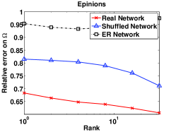
(a) Epinions

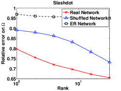
(b) Slashdot

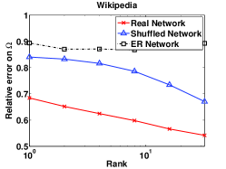
(c) Wikipedia

Figure 2: Relative error on $\Omega$, the observed entries, between adjacency matrix and completed matrix, for real-life networks versus random networks. Real-life networks achieve much smaller relative error for every $k$ as compared with random networks.

6.3 Sign Prediction

We now compare the performance of our proposed methods for sign prediction. As introduced in Sections 3 and 4, there are two families of cycle-based methods: one based on measures of imbalance (MOI), and the other based on the supervised learning using higher order cycles (HOC). Both families depend on a parameter $\ell\geq 3$ that denotes the order of the cycles that the method is based on. For MOI, we consider all $\ell$ less than $10$ as well as $\infty$ (recall that in this case MOI becomes Katz measure), and for HOC we consider $\ell=3,4,5$. Note that the set of features used by HOC-$(\ell+1)$ is a strict superset of the features used by HOC-$\ell$.

We also consider two fully global approaches for low rank matrix completion – Singular Value Projection from Section 5.2 and matrix factorization from Section 5.3. The SVP approach (denoted as LR-SVP) is chosen to demostrate that perfect recovery can be achieved if the observations are uniformly distributed. For matrix factorization, we consider the ALS method that solves problem (20), as well as SGD methods that solve the general problem (21) with sigmoid loss and square-hinge loss, defined in (22). We denote these methods as LR-ALS, LR-SIG and LR-SH, respectively.

6.3.1 Synthetic Datasets

We first compare all categories of approaches on synthetic datasets. We choose LR-SVP, LR-ALS, MOI-$\infty$ and HOC-3 as representatives of the two approaches of low rank matrix completion, MOI-based, and HOC-based methods respectively. We consider the underlying network $A^{\star}$ to be a complete $5$-weakly balanced network, where the five clusters have sizes $100$, $200$, $300$, $400$ and $500$. Instead of observing all of $A^{\star}$, we assume that we only observe a partial network $A$ by sampling some entries from $A^{\star}$ using three sampling procedures: uniform sampling, uniform sampling with noise, and sampling with power-law distribution. For each algorithm, we input the observed entries as training data and calculate the sign prediction accuracy on the rest of the entries.

Uniform sampling: In this scenario, we generate several observed networks $A=A^{\star}(s,0,\mathcal{D}_{\textrm{uni}})$. We vary $s$ from $0.001$ to $0.1$ and plot the prediction accuracy in Figure 3a. Under this setting, LR-SVP and LR-ALS outperform the cycle-based methods. We observe that MOI-$\infty$ performs the worst with accuracy only 50%-70%. However, if we repeat the same experiment substituting $A^{\star}$ with $A^{\star}_{2}$, where $A^{\star}_{2}$ is a complete strongly balanced network whose two groups have size $1000$, we observe that MOI and global methods perform alike as shown in Figure 3b. This is because MOI uses cycle-based measurements to make more cycles become balanced. This prediction policy is most appropriate when $k=2$ (that is, the underlying network $A^{\star}$ has strong balance), but performs poorly when the underlying network is weakly balanced (i.e. more than two groups). HOC-3 works much better than MOI-$\infty$ since it learns a classifier from cycle-based features rather than simply making cycles balanced, but its accuracy drops dramatically when $s$ is less than $0.05$. On the other hand, both LR-SVP and LR-ALS show high accuracy for all $s\geq 0.01$. In particular, LR-SVP can achieve 100% accuracy when $s>0.07$, which reconfirms the theoretical recovery guarantee stated in Theorem 18. Moreover, although LR-ALS has no theoretical guarantee, it can still recover the ground truth, an observation that is consistent with previous results.

Uniform sampling with noise: To make the synthetic data more similar to real data, we further add noise into observations. We generate observed networks $A=A^{\star}(0.1,\epsilon,\mathcal{D}_{\textrm{uni}})$, where $\epsilon$ varies from $0.01$ to $0.25$. The result is shown in Figure 3c. We can see that global methods are still clearly better than cycle-based methods when noise level becomes higher. Moreover, LR-SVP perfectly recovers $A^{\star}$ when the noise level $\epsilon<0.05$, and LR-ALS also achieves perfect recovery with a smaller $\epsilon$.

Sampling with power-law distribution: As Sections 5.1 and 5.2 stated, the exact recovery guarantees of convex relaxation and SVP for matrix completion crucially rely on the assumption that observed entries are uniformly sampled. However, in most real networks (for example, Slashdot in Kunegis et al. (2009)), the degree distribution of observed entries follows a power law. Therefore, we examine how the approaches perform on power-law distributed networks. The power-law distributed networks are generated using the Chung-Lu-Vu (CLV) model proposed by Chung et al. (2004), which allows one to generate random graphs with arbitrary expected degree sequence. Similar to the uniform sampling case, we perform the sign prediction task on $A=A^{\star}(s,0,\mathcal{D}_{\textrm{pow}})$ varying $s$ from $0.001$ to $0.1$, and plot the prediction accuracy in Figure 3d. We can see that MOI-$\infty$ still has poor performance for weakly balanced graphs. However, unlike the uniform sampling case, LR-SVP has lower accuracy rate compared to HOC-3 when $s<0.1$. On the other hand, LR-ALS still performs better than all other methods in power-law distributed graphs.

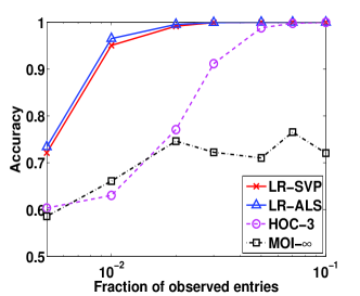
(a) Uniformly sampled without noise ($k=5$)

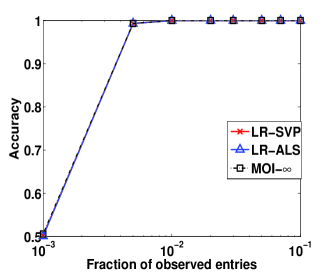
(b) Uniformly sampled without noise on balanced networks ($k=2$)

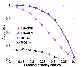
(c) Uniformly sampled with noise ($k=5$)

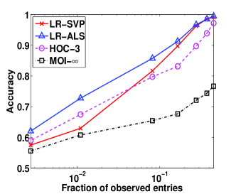
(d) Power-law distributed networks ($k=5$)

Figure 3: Sign prediction accuracy of local and global methods on synthetic datasets. On (strongly) balanced networks (3b), MOI-$\infty$ is seen to perform as well as LR-SVP and LR-ALS. However, in general weakly balanced networks, global methods LR-SVP and LR-ALS outperform cycle-based methods such as MOI-$\infty$ and HOC-3. In addition, LR-ALS is more robust than LR-SVP when the observations are sampled from a power-law distribution.

From results on synthetic data shown in Figure 3, we can conclude that global methods generally do better than local methods on synthetic setting, and the low rank model with matrix factorization (LR-ALS) performs the best in most cases, even when observed entries are not uniformly distributed.

6.3.2 Real-life Datasets

Now we further evaluate our sign prediction methods on three real-life networks. To begin with, we evaluate and compare MOI methods using a leave-one-out type methodology: each edge in the network is successively removed and the method tries to predict the sign of that edge using the rest of the network. Figure 4 shows the accuracy of MOI based methods. Note that the accuracy is shown for edges with embeddedness under a certain threshold. First, we see that the accuracy is a non-decreasing function of the embeddedness threshold. Next, it is clear that higher-order methods perform significantly better than MOI-$3$ (triangles) method. Finally, the performance boost is larger for edges with low embeddedness. This is expected as edges of low embeddedness by definition do not have many common neighbors for their end-points, and higher-order cycles have relatively better information for such edges than others. We also observe from our experiments that beyond $\ell=5$, the performance gain is not very significant.

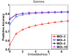
(a) Epinions

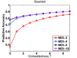
(b) Slashdot

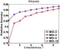
(c) Wikipedia

Figure 4: Accuracy of Measures of Imbalance (MOI) Based Methods for $\ell=3,4,5,10.$ These plots show the accuracy of MOI-$\ell$ methods for edges with embeddedness at least $T$ for various thresholds $T$. We see that the difference in the performance of MOI-$3$ and higher order methods is larger when edges with lower embeddedness are considered. We also see that the improvement obtained by going beyond order $5$ is not very significant.

Next, we compare HOC methods. We resort to $10$-fold cross-validation. To be more concrete, we (randomly) created $10$ disjoint test folds each consisting of $10\%$ of the total number of edges in the network. For each test fold, the remaining $90\%$ of the edges serve as the training set. For a given test fold, the feature extraction and logistic model training happen on a graph with the test edges removed. To evaluate HOC methods, we consider not only prediction accuracies but also false-positive rates. We report both accuracies and false-positive rates by averaging them over the $10$ folds. As shown in Table 6, in all the datasets, there is a small improvement in accuracy by using higher order cycles (HOC-$5$). The false positive rate, however, reveals a more interesting phenomenon in Figure 5. Indeed, higher order methods (such as HOC-$5$) significantly reduce the false positive rate as compared to that of HOC-$3$. However Figure 5 shows that, unlike MOI based methods, edge embeddedness does not seem to affect the decrease in false positive rate for HOC methods. We see this trend across all the datasets.

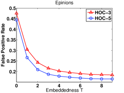
(a) Epinions

(b) Slashdot

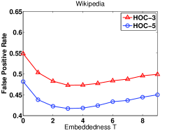
(c) Wikipedia

Figure 5: False Positive Rates of Higher Order Cycle (HOC) Methods for $\ell=3,5.$ These plots show the false positive rate of HOC-$\ell$ methods for edges with embeddedness at least $T$ for various thresholds $T$. We see that considering higher order cycles has the benefit of significantly reducing false-positives while simultaneously achieving slightly better overall accuracy (refer to Table 6). However, unlike what we see for MOI methods, here the improvement does not seem to depend strongly on edge embeddedness. The false positive rates for HOC-$4$ are very similar to that of HOC-$5$ and hence are not shown for clarity.

At this point, we see that for cycle-based methods, considering higher order cycles benefits the accuracy of sign prediction and lowers the false positive rate. Furthermore, the results are consistent across the three diverse networks. These results confirm the intuition that getting more global information improves quality of prediction, and motivate us to consider the fully global structure of networks.

Now we turn our attention to low rank modeling approaches. We have seen that LR-SVP fails to perform well under power-law distributions of observed relationships in synthetic networks (see Figure 3d), so we consider the more robust matrix factorization approach for solving the matrix completion problem, including LR-ALS, LR-SIG and LR-SH, for experiments on real datasets. Again, we use $10$-fold cross validation setting, and report the average prediction accuracy for each dataset in Table 6. From the table, we observe that global methods clearly outperform cycle-based methods. In particular, we observe that HOC-5 only improves HOC-3 by less than 1.5%, while global methods consistently improve the accuracy of HOC-5 by more than 2% over all datasets. In addition, LR-SIG and LR-SH further improve the accuracy of LR-ALS. This shows that the sigmoid and square-hinge loss are more suitable for sign prediction, which supports the discussion in Section 5.3.

Table 6: The sign prediction accuracy for low rank modeling methods and cycle-based methods. We can see that the low rank modeling approaches are better than cycle-based methods.

	MOI-3	MOI-10	HOC-3	HOC-5	LR-ALS	LR-SIG	LR-SH
Epinions	0.5539	0.8497	0.9014	0.9080	0.9374	0.9465	0.9437
Slashdot	0.3697	0.7850	0.8303	0.8469	0.8774	0.8789	0.8835
Wikipedia	0.7456	0.8220	0.8424	0.8605	0.8814	0.8830	0.8810

In Figure 6, we further select a representative of each category, MOI-10, HOC-5 and LR-ALS, and show their performance with different levels of edge embeddedness (LR-SIG and LR-SH perform similar to LR-ALS among all datasets). One might expect that cycle-based approaches should perform better on edges with higher embeddedness because more cycle information is available. However, surprisingly LR-ALS achieves higher prediction accuracy regardless of the embeddedness. All above results show that global methods are more effective than local methods.

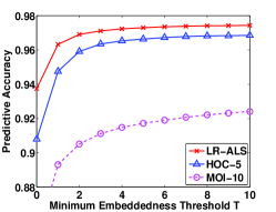
(a) Epinions

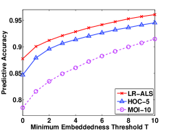
(b) Slashdot

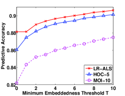
(c) Wikipedia

Figure 6: Sign prediction accuracy of local and global methods with different levels of embeddedness. These plots show the accuracy for edges with embeddedness at least $T$. We can see that LR-ALS consistently achieves the highest accuracy for all thresholds $T$.

6.3.3 Running Time Comparison

In addition to prediction accuracy, we now compare the running time required by the different methods. As discussed in Section 5.3, low rank modeling with matrix factorization is more efficient than cycle-based algorithms in terms of time complexity. Here, we further show that matrix factorization methods are empirically much faster than cycle-based algorithms. The running times are summarized in Table 7. To conduct timing tests on a large signed network, in addition to the three real datasets as described in Table 4, we construct a large-scale synthetic dataset called Cluster10 where the number of edges is 100 times more than Epinions. Cluster10 is generated from a $10$-weakly balanced network, in which clusters have sizes 20000, 40000, …, 200000. There are totally 1.1 million nodes and 120 million edges uniformly sampled from the complete graph. We construct this synthetic data to show that our matrix factorization approach can easily scale up to massive graphs compared to HOC methods. For matrix factorization approach, we report the time needed to solve the model by SGD (with sigmoid and square-hinge) and ALS (with square loss). For HOC methods which build classifiers from cycle-based features, since the time for training phase depends on the classifier, we only report the time for computation of features. Thus the reported time for HOC is an underestimate of the time required to construct the HOC model; even then we can see that the time required by LR-ALS, LR-SIG and LR-SH is much lower than HOC methods.

In conclusion, for the sign prediction problem, we see that considering fully global structure of networks gives us the best results. In particular, the low rank model with matrix factorization is clearly the most competitive method in terms of accuracy and scalability.

Table 7: Running time (in seconds) for low rank model with matrix factorization and HOC on real datasets and a 1.1 million node synthetic data Cluster10. The time of LR-SGD is the average time of LR-SIG and LR-SH. For HOC methods, we only consider the time for feature computation before the model training, while for LR methods we report the total time for constructing the model. We can see that LR methods with matrix factorization are clearly more efficient than cycle-based algorithms.

	HOC-3	HOC-4	HOC-5	LR-ALS	LR-SGD
Wikipedia	18.08	74.52	462.92	2.26	2.41
Slashdot	133.4	1,936.0	$>10,000$	17.4	24.7
Epinions	560.64	6,156.8	$>10,000$	28.67	37.2
Cluster10	$>10,000$	$>10,000$	$>10,000$	455.1	1,152

6.4 Clustering

In this subsection, we show that our clustering approach, which completes the low-rank structure of signed networks before performing clustering, outperforms spectral clustering based on the signed Laplacian (Kunegis et al., 2010). We conduct experiments on synthetic data generated from weakly balanced networks (note that we do not have ground truth for clustering in the real-life datasets). We consider a $10$-weakly balanced network $A^{\star}$ where size of each group is $100$, and observe entries from $A^{\star}$ with two sampling procedures: uniform sampling and uniform sampling with noise.

To measure the performance of clustering, we calculate the number of edges that satisfy the ground-truth clustering, which is defined by

$$\sum_{i,j:s_{i}=s_{j}}I(\bar{s_{i}}=\bar{s_{j}})+\sum_{i,j:s_{i}\neq s_{j}}I(\bar{s_{i}}\neq\bar{s_{j}}).$$ (25)

where $s_{1},\dots,s_{n}$ denote the ground-truth clustering assignment for each node, and $\bar{s}_{1},\dots,\bar{s}_{n}$ are the clustering results given by the clustering algorithm.

Following the procedure outlined in the previous subsection, in the uniform sampling case, we consider the networks $A=A^{\star}(s,0,\mathcal{D}_{\textrm{uni}})$ with $s\in[0.01,0.06]$, while in sampling with noise case we consider networks $A=A^{\star}(0.1,\epsilon,\mathcal{D}_{\textrm{uni}})$ with $\epsilon\in[0.01,0.06]$. For each observed network, we apply Algorithm 2 (See Section 5.5) and clustering via the signed Laplacian, and evaluate clustering results using (25). The results of these two scenarios are shown in Figure 7. In both the scenarios, our proposed clustering approach is significantly better than clustering based on the signed Laplacian. This shows that recovering the low-rank structure of signed networks leads to improved clustering results.

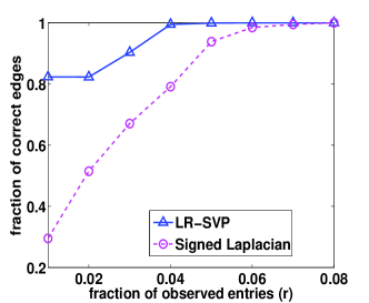
(a) Data without noise

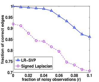
(b) Data with noise

Figure 7: Clustering partially observed synthetic data. Figure 7a is the result without noise and Figure 7b is the result with noise. In both cases, clustering with LR-SVP performs significantly better than clustering with signed Laplacian.

7 Related Work

Signed networks have been studied since the early 1950s. Harary and Cartwright were the first to mathematically study structural balance. They defined balanced triads and proved the global structure of balanced signed networks (Harary, 1953; Cartwright and Harary, 1956). Davis (1967) further generalized the balance notion to weak balance by allowing triads with all negative edges, and showed that weakly balanced graphs have mutual antagonistic groups as global structure.

Though theoretical studies of signed networks have been conducted for a long time, it was not until this decade that analysis of real signed networks could be done at a large scale as large real networks have become more accessible recently. For example, Kunegis et al. (2009) performed several analysis tasks on Slashdot, and Leskovec et al. (2010a, b) studied the local and global structure of three real signed networks. They designed several computational experiments to justify that the structure of these signed networks match some widely believed social theories.

In this paper, we focused on problems in signed networks. However, these problems have their counterparts in unsigned networks. For instance, structural link prediction in unsigned networks corresponds to the sign prediction problem. Structural link prediction has been well explored, and it is usually solved by computing a similarity measure between nodes (Liben-Nowell and Kleinberg, 2007), such as those proposed by Katz (1953) and Adamic and Adar (2003). The sign prediction problem, however, was not formally considered until the work by Guha et al. (2004), in which they develop a trust propagation framework to predict trust or distrust between entities. More recently, Kunegis et al. (2009, 2010) reconsidered this problem by using various similarity functions and kernels such as matrix exponential and signed Laplacian. Leskovec et al. (2010a) proposed a machine learning formulation of this problem, arguing that learning from only local triangular structure of edges can achieve reasonable accuracy.

Sign prediction using our global method is closely related to the low-rank matrix completion problem. In the last five years, there has been substantial research studying exact recovery conditions for this problem (Candés and Recht, 2008; Candés and Tao, 2009), and algorithms with theoretical guarantees have also been proposed, such as SVT (Cai et al., 2010) and SVP (Jain et al., 2010). Matrix factorization is another approximation technique for matrix completion. Though this approach is notoriously hard to analyze, it is very competitive in practice (Koren et al., 2009). While the matrix completion problem has been considered mostly in collaborative filtering, our low rank model arises naturally from the weak balance of signed networks.

Clustering is another fundamental problem in network analysis. For unsigned networks, there are several proposed algorithms that have been shown to be effective, such as clustering via graph Laplacian (Ng et al., 2001), modularity (Newman, 2006) and multilevel approaches (Dhillon et al., 2007). However, most of these approaches can not be directly extended to signed networks since weak balance theory does not apply to unsigned networks. As a result, researchers have tried to tailor unsigned network clustering algorithms in order to make them applicable to signed networks. For instance, Doreian and Mrvar (1996) proposed a local search strategy which is similar to the Kernighan-Lin algorithm (Kernighan and Lin, 1970). Starting with an initial clustering assignment, it tries to move nodes one by one to get a more preferable clustering. Yang et al. (2007) proposed an agent-based method which basically conducts a random walk on the graph. Kunegis et al. (2010) generalized spectral algorithms to signed networks. They proposed a spectral approach using the so-called “signed” Laplacian, and showed that partitioning signed networks into two groups using the signed Laplacian kernel is analogous to considering ratio cut on unsigned networks. Anchuri and Magdon-Ismail (2012) proposed hierarchical iterative methods that solve 2-way signed modularity objectives using spectral relaxation at each hierarchy. Chiang et al. (2012) proposed some graph kernels for signed network clustering, and showed that the multilevel framework can be extended to this problem.

Another line of research on signed graph clustering problem is correlation clustering. Correlation clustering is motivated from document classification: given a set of documents with some pairs of documents labeled similar or different, the goal is to find a partition such that documents in the same cluster are mostly similar (Bansal et al., 2004). The problem was first considered by Bansal et al. (2004), who proved that the problem is NP-hard to optimize, and proposed two approximation algorithms to maximize the “agreement” (defined as the number of edges that are correctly classified under a partition) and minimize the “disagreement” (defined vice versa) under the special case that all pairwise label information is given. The bounds for general correlation clustering setting were provided by Dmaine et al. (2006). On the other hand, some researchers have also considered the correlation clustering problem from the statistical learning theory viewpoint. For example, Joachims and Hopcroft (2005) give error bounds for the problem if only partial pairs are observed. Recently, Cesa-Bianchi et al. (2012) proposed a method for sign prediction by learning a correlation clustering index. They consider three types of learning models: batch, online and active learning, and provide theoretical bounds for prediction mistakes under each setting.

8 Conclusions and Future Work

In this paper, we studied the usefulness of social balance on signed networks, with two fundamental applications: sign prediction and clustering. Starting from a local view of social balance, we proposed two families of sign prediction methods based on local triads and cycles: prediction via measures of social imbalance (MOIs) and supervised learning based on high order cycles (HOCs). For both approaches, predictive accuracies are improved if longer cycles are taken into consideration, suggesting that a broader view of local patterns helps in sign prediction. We then considered the fully global perspective on social balance, and showed that the adjacency matrices of balanced networks are low rank. Based on this observation, we modeled the sign prediction problem as a low-rank matrix completion problem. We discussed three approaches to matrix completion: convex relaxation, singular value projection, and matrix factorization. In addition, we applied this low rank modeling technique to the clustering problem. In experiments, we observe that sign prediction via matrix factorization not only outperforms MOIs and HOCs, but requires much less running time. Clustering results are also more favorable via the matrix completion approach in comparison with the existing signed Laplacian approach. All of these results consistently demonstrate the effectiveness of the global viewpoint of social balance.

For future work, one possible direction is to explore analysis tasks on heterogeneous signed networks. Since there are different types of entities in heterogeneous networks, currently there are no clear answers to questions such as: do balance relationships exist on such networks? How do we quantitatively measure balance if balance patterns exist? How is balance at a local level related to the global structure? Furthermore, another possible direction is to examine other theories for analysis tasks on signed networks. For example, some recent work (Leskovec et al., 2010a, b) has considered status theory. While Leskovec et al. (2010a) found evidence that status theory holds in general in real signed networks, patterns conforming to status theory are quite different from those conforming to balance theory. Thus, it is natural to ask how to design algorithms by pursuing global patterns conforming to status theory. These interesting directions are worth exploring in future research.

9 Acknowledgments

We gratefully acknowledge the support of NSF under grants CCF-0916309, CCF-1117055, and of DOD Army under grant W911NF-10-1-0529. Most of the contribution of Ambuj Tewari to this work occurred while he was a postdoctoral fellow at the University of Texas at Austin.

References

- Adamic and Adar (2003) Lada A. Adamic and Eytan Adar. Friends and neighbors on the web. Social Networks, 25(3):211–230, 2003.
- Anchuri and Magdon-Ismail (2012) Pranay Anchuri and Magdon-Ismail. Communities and balance in signed networks: A spectral approach. In IEEE/ACM International Conference on Advances in Social Networks Analysis and Mining, 2012.
- Bansal et al. (2004) Nikihil Bansal, Avrim Blum, and Shuchi Chawla. Correlation clustering. Machine Learning, 56:89–113, 2004.
- Cai et al. (2010) Jian-Feng Cai, Emmanuel J. Candés, and Zuowei Shen. A singular value thresholding algorithm for matrix completion. Society for Industrial and Applied Mathematics (SIAM), 20(4):1956–1982, 2010.
- Candés and Recht (2008) Emmanuel J. Candés and Benjamin Recht. Exact matrix completion via convex optimization. Found. of Comput. Math., 9:712–772, 2008.
- Candés and Tao (2009) Emmanuel J. Candés and Terence Tao. The power of convex relaxation: Near-optimal matrix completion. IEEE Trans. Inform. Theory, 56(5):2053–2080, 2009.
- Cartwright and Harary (1956) Dorwin Cartwright and Frank Harary. Structure balance: A generalization of Heider’s theory. Psychological Review, 63(5):277–293, 1956.
- Cesa-Bianchi et al. (2012) Nicolo Cesa-Bianchi, Claudio Gentile, Fabio Vitale, , and Giovanni Zappella. A correlation clustering approach to link classification in signed networks. In COLT, 2012.
- Chiang et al. (2011) Kai-Yang Chiang, Nagarajan Natarajan, Ambuj Tewari, and Inderjit S. Dhillon. Exploiting longer cycles for link prediction in signed networks. In CIKM, 2011.
- Chiang et al. (2012) Kai-Yang Chiang, Joyce JiYoung Whang, and Inderjit S. Dhillon. Scalable clustering of signed networks using balance normalized cut. In CIKM, 2012.
- Chung et al. (2004) Fan Chung, Linyuan Lu, and Van Vu. Spectra of random graphs with given expected degrees. Internet Mathematics, 1, 2004.
- Davis (1967) James A. Davis. Clustering and structural balance in graphs. Human Relations, 20(2):181–187, 1967.
- Dhillon et al. (2007) Inderjit S. Dhillon, Yuqiang Guan, and Brian Kulis. Weighted graph cuts without eigenvectors: A multilevel approach. IEEE Trans. on Pattern Analysis and Machine Intelligence, 29(11):1944–1957, 2007.
- Dmaine et al. (2006) Erik D. Dmaine, Dotan Emanuel, Amos Fiat, and Nicole Immorlica. Correlation clustering in general weighted graphs. Theoretical Computer Science, 361(2-3):172–187, 2006.
- Doreian and Mrvar (1996) Patrick Doreian and Andrej Mrvar. A partitioning approach to structural balance. Social Networks, 18(21):149–168, 1996.
- Erdös and Rényi (1960) P. Erdös and A. Rényi. On the evolution of random graphs. In Publication of the mathematical institute of the Hungarian academy of sciences, pages 17–61, 1960.
- Fazel et al. (2001) Maryam Fazel, Haitham Hindi, and Stephen P. Boyd. A rank minimization heuristic with application to minimum order system approximation. In American Control Conference, volume 6, pages 4734–4739, 2001.
- Guha et al. (2004) R. V. Guha, Ravi Kumar, Prabhakar Raghavan, and Andrew Tomkins. Propagation of trust and distrust. In WWW, 2004.
- Harary (1953) Frank Harary. On the notion of balance of a signed graph. Michigan Mathematical Journal, 2(2):143–146, 1953.
- Hsieh et al. (2012) Cho-Jui Hsieh, Kai-Yang Chiang, and Inderjit S. Dhillon. Low rank modeling of signed networks. In KDD, 2012.
- Jain et al. (2010) Patreek Jain, Reghu Meka, and Inderjit Dhillon. Guaranteed rank minimization via singular value projection. In NIPS, pages 934–945, 2010.
- Joachims and Hopcroft (2005) Thorsten Joachims and John Hopcroft. Error bounds for correlation clustering. In Proceedings of the 22nd international conference on Machine learning, ICML ’05, New York, NY, USA, 2005. ACM.
- Karp (1972) Richard M. Karp. Reducibility among combinatorial problems. In Complexity of Computer Computations (1972), page 85=103, 1972.
- Katz (1953) Leo Katz. A new status index derived from sociometric analysis. Psychometrika, 18(1):39–43, 1953.
- Kernighan and Lin (1970) Brian W. Kernighan and Shen Lin. An efficient heuristic procedure for partitioning graphs. Bell system technical journal, 49(1):291–307, 1970.
- Koren et al. (2009) Yehuda Koren, Robert M. Bell, and Chris Volinsky. Matrix factorization techniques for recommender systems. IEEE Computer, 42:30–37, 2009.
- Kunegis et al. (2009) Jérôme Kunegis, Andreas Lommatzsch, and Christian Bauckhage. The slashdot zoo: Mining a social network with negative edges. In WWW, pages 741–750, 2009.
- Kunegis et al. (2010) Jérôme Kunegis, Stephan Schmidt, Andreas Lommatzsch, Jürgen Lerner, Ernesto W. DeLuca, and Sahin Albayrak. Spectral analysis of signed graphs for clustering, prediction and visualization. In SDM, pages 559–570, 2010.
- Leskovec et al. (2010a) Jure Leskovec, Daniel Huttenlocher, and Jon Kleinberg. Predicting positive and negative links in online social networks. In Proceedings of the 19th International Conference on World Wide Web, pages 641–650, 2010a.
- Leskovec et al. (2010b) Jure Leskovec, Daniel Huttenlocher, and Jon Kleinberg. Signed networks in social media. In CHI, 2010b.
- Liben-Nowell and Kleinberg (2007) David Liben-Nowell and Jon Kleinberg. The link-prediction problem for social networks. Journal of the American Society for Information Science and Technology, 58(7):1019–1031, 2007.
- Newman (2006) M. E. J. Newman. Modularity and community structure in networks. Proceedings of the National Academy of Sciences of USA, 103(23):8577–8582, 2006.
- Ng et al. (2001) Andrew Y. Ng, Michael I. Jordan, and Yair Weiss. On spectral clustering: analysis and an algorithm. In NIPS, pages 849–856. MIT Press, 2001.
- van de Rijt (2011) Arnout van de Rijt. The micro-macro link for the theory of structural balance. Journal of Mathematical Sociology, 35(1):94–113, 2011.
- Yang et al. (2007) Bo Yang, William Cheung, and Jiming Liu. Community mining from signed social networks. IEEE Trans. on Knowledge and Data Engineering, 19(10):1333–1348, 2007.