Rational approximations of spectral densities
based on the Alpha divergence

Abstract

We approximate a given rational spectral density by one that is consistent with prescribed second-order statistics. Such an approximation is obtained by selecting the spectral density having minimum “distance” from under the constraint corresponding to imposing the given second-order statistics. We analyze the structure of the optimal solutions as the minimized “distance” varies in the Alpha divergence family. We show that the corresponding approximation problem leads to a family of rational solutions. Secondly, such a family contains the solution which generalizes the Kullback-Leibler solution proposed by Georgiou and Lindquist in 2003. Finally, numerical simulations suggest that this family contains solutions close to the non-rational solution given by the principle of minimum discrimination information.

1 Introduction

This paper deals with the rational approximation of power spectra of stationary stochastic processes. More precisely, we consider the following situation. Let $y=\left\{y_{k};\;k\in\mathbb{Z}\right\}$ be a zero mean, $\mathbb{R}$-valued, purely non-deterministic, full-rank, stationary process with unknown spectral density $\Omega(\mathrm{e}^{j\vartheta})$ defined on the unit circle $\mathbb{T}$. A rational prior spectral density $\Psi\in\mathbb{S}_{+}(\mathbb{T})$, which represents the a priori information on $y$, is available. Here, $\mathbb{S}_{+}(\mathbb{T})$ denotes the family of bounded and coercive $\mathbb{R}$-valued spectral density functions on $\mathbb{T}$. Then, some second-order statistics of $y$ are observed. These are encoded in the output covariance, denoted by $\Sigma$, of a rational filters bank $G(z)=(zI-A)^{-1}B$ driven by $y$. The filter parameters are chosen in such a way that $A\in\mathbb{R}^{n\times n}$ is a stability matrix, $B\in\mathbb{R}^{n}$, and $(A,B)$ is a reachable pair with $n>1$. Thus the output process, denoted by $x=\{x_{k};\;k\in\mathbb{Z}\}$, is a stationary process, and $\Sigma=\mathbb{E}[x_{k}x_{k}^{T}]=\int G\Omega G^{*}$ is a positive definite matrix. Here, integration takes places on $[-\pi,\pi)$ with respect to the normalized Lebesgue measure $\mathrm{d}\vartheta/2\pi$. The rational prior $\Psi$ is typically inconsistent with $\Sigma$, i.e. $\Sigma\neq\int G\Psi G^{*}$. Hence, our task consists in finding a rational spectral density $\Phi\in\mathbb{S}_{+}(\mathbb{T})$ which is as close as possible to $\Psi$ and such that

$$\Sigma=\int G\Phi G^{*}.$$ (1)

The closeness between $\Phi$ and $\Psi$ is quantified by considering a distance measure $\mathcal{S}(\cdot\|\cdot)$ among spectral densities in $\mathbb{S}_{+}(\mathbb{T})$, i.e. $\mathcal{S}(\Phi_{1}\|\Phi_{2})\geq 0$ for each $\Phi_{1},\Phi_{2}\in\mathbb{S}_{+}(\mathbb{T})$ and equality holds if and only if $\Phi_{1}=\Phi_{2}$ but we do not require that symmetry and triangular inequality hold. In other words we reconcile the inconsistency among $\Sigma$ and $\Psi$ by approximating the spectrum $\Psi$ by a rational spectrum $\Phi$ compatible with $\Sigma$. This problem is motivated by THREE-like spectral estimation paradigms [5, 18, 20, 11, 21, 13, 9, 22] wherein $\Phi$ represents an estimate of the unknown spectral density $\Omega$ compatible with the given second-order statistics of $\Omega$ and as close as possible to the a priori information given.

The role of the filters bank $G(z)$ consists in providing the interpolation conditions for the solution to the spectrum approximation problem. More specifically, by choosing the filters bank poles appropriately, it is possible to give preference to selected frequency bands of $\Phi$ and allow more accurate reconstruction of $\Omega$ in these particular frequency bands, [5].

Concerning the distance measures in the above problem, we have many options. In [18], the Kullback-Leibler divergence among spectral densities having the same zeroth moment is considered

$$\mathcal{S}_{\mathrm{KL0}}(\Phi_{1}\|\Phi_{2}):=\int\Phi_{1}\log\left(\frac{\Phi_{1}}{\Phi_{2}}\right).$$ (2)

The found rational solution $\Phi$ is the spectral density satisfying (1) which minimizes $\mathcal{S}_{\mathrm{KL0}}(\Psi\|\Phi)$. Note that in statistics, information theory and communications, the Kullback-Leibler divergence is typically minimized with respect to the first argument, [7, 8], according to the Principle of minimum discrimination information, MinxEnt, [19]. It states that, given new information, a new distribution $\Phi$ should be chosen in such a way as to minimize $\mathcal{S}_{\mathrm{KL0}}(\Phi\|\Psi)$. In [18], the unusual choice to minimize with respect to the second argument is dictated by the fact that the optimization of $\mathcal{S}_{\mathrm{KL0}}(\Phi\|\Psi)$ leads to a non-rational “exponential-type” solution, [17]. Then, in [11] and [9], the rational solutions corresponding to the Hellinger distance and the Itakura-Saito distance, respectively, are considered. Finally, in [22] the Beta divergence family is considered. The latter smoothly connects the Kullback-Leibler divergence with the Itakura-Saito distance. Making additional assumptions on $\Psi$ besides the rationality, it is possible to prove that the Beta divergence leads to a family of rational solutions. Finally, it is worth noting that the solutions considered in [11, 9, 22] also hold for the multichannel case, i.e. $y$ is a multivariate process.

The aim of this paper is to solve the previous spectrum approximation problem by employing the Alpha divergence family which smoothly connects the Kullback-Leibler divergence

$$\mathcal{S}_{\mathrm{KL}}(\Phi_{1}\|\Phi_{2}):=\int\Phi_{1}\log\left(\frac{\Phi_{1}}{\Phi_{2}}\right)-\Phi_{1}+\Phi_{2}$$ (3)

with its reverse $\mathcal{S}_{\mathrm{KL}}(\Phi_{2}\|\Phi_{1})$, passing through the Hellinger distance. Firstly we will generalize the solution in [18] to spectral densities with different zeroth moment. Then, we will see that it is possible to characterize a family of rational solutions to the problem without making additional assumptions on $\Psi$. The limit of this family of solutions has the same “exponential-type” structure as the MinxEnt solution. Furthermore, simulations suggest that the limit above converges to the non-rational solution given by $\mathcal{S}_{\mathrm{KL}}(\Phi\|\Psi)$. Thus, the spectrum approximation problem based on the Alpha divergence family also seems to provide rational solutions, for a suitable choice of the $\alpha$ parameter, close to the MinxEnt solution.

2 Spectrum approximation problem and feasibility conditions

The spectrum approximation problem we are dealing with minimizes a suitable distance measure, denoted by $\mathcal{S}(\Phi\|\Psi)$, over the set

$$\mathcal{I}_{\Sigma}:=\left\{\Phi\in\mathbb{S}_{+}(\mathbb{T})\;|\;\int G\Phi G^{*}=\Sigma\right\}$$ (4)

where $\Psi\in\mathbb{S}_{+}(\mathbb{T})$ is rational, and $G(z)=(zI-A)^{-1}B$ has the same properties specified in the Introduction. Both $\Psi$ and $G(z)$ are given. The output covariance $\Sigma$ is estimated by a given finite-length sequence $y_{1}\ldots y_{N}$, extracted from a realization of $y$, see [12, 23]. Thus, the first problem concerns the feasibility of the spectrum approximation problem, i.e. when the set $\mathcal{I}_{\Sigma}$ is non-empty for a given $\Sigma$. To deal with this issue, we first introduce some notation: $\mathcal{Q}_{n}\subset\mathbb{R}^{n\times n}$ denotes the $n(n+1)/2$-dimensional real vector space of $n$-dimensional symmetric matrices and $\mathcal{Q}_{n,+}$ denotes the corresponding cone of positive definite matrices. We denote as $\mathcal{V}(\mathbb{S}_{+}(\mathbb{T}))$ the linear space generated by $\mathbb{S}_{+}(\mathbb{T})$. Finally, we introduce the linear operator

$$\Gamma : \mathcal{V}(\mathbb{S}_{+}(\mathbb{T}))\rightarrow\mathcal{Q}_{n}$$ (5)

$$\Phi\mapsto\int G\Phi G^{*}.$$

In [16], it was shown that a matrix $P\in\mathcal{Q}_{n}$ belongs to the range of $\Gamma$, denoted by $\mathrm{Range}\;\Gamma$, if and only if there exists $H\in\mathbb{R}^{1\times n}$ such that

$$P-APA^{T}=BH+H^{T}B^{T}.$$ (6)

It turns out that the spectrum approximation problem is feasible if and only if $\Sigma\in\mathrm{Range}\;\Gamma\cap\mathcal{Q}_{n,+}$, see [16, 11]. Once we have $\Sigma$ in such a way that the spectrum approximation problem is feasible, we can replace $G$ with $\overline{G}=\Sigma^{-\frac{1}{2}}G$ and $(A,B)$ with $(\overline{A}=\Sigma^{-\frac{1}{2}}A\Sigma^{\frac{1}{2}},\overline{B}=\Sigma^{-\frac{1}{2}}B)$. Thus, constraint (1) may be rewritten as

$$\int\bar{G}\Phi\bar{G}^{*}=I.$$ (7)

Accordingly, from now on we assume that our spectrum approximation problem is feasible and we consider the following equivalent formulation: Given a rational prior $\Psi\in\mathbb{S}_{+}(\mathbb{T})$ and $G(z)$ such that $I\in\mathrm{Range}\;\Gamma$, minimize $\mathcal{S}(\Phi\|\Psi)$ over the (non-empty) set

$$\left\{\Phi\in\mathbb{S}_{+}(\mathbb{T})\;|\;\int G\Phi G^{*}=I\right\}.$$ (8)

In the following section we will introduce the last element characterizing our problem: The distance measure $\mathcal{S}(\Phi\|\Psi)$.

3 Spectrum approximation problem with the Alpha divergence

The Alpha divergence family, [1, 6], among two spectral densities $\Phi_{1},\Phi_{2}\in\mathbb{S}_{+}(\mathbb{T})$ is defined as

$$\mathcal{S}_{\alpha}(\Phi_{1}\|\Phi_{2}):=\int\frac{1}{\alpha(\alpha-1)}\Phi_{1}^{\alpha}\Phi_{2}^{1-\alpha}-\frac{1}{\alpha-1}\Phi_{1}+\frac{1}{\alpha}\Phi_{2}$$ (9)

where $\alpha$ is a real parameter. For $\alpha=0$ and $\alpha=1$, it is defined by continuity

$$\lim_{\alpha\rightarrow 0}\mathcal{S}_{\alpha}(\Phi_{1}\|\Phi_{2})=\mathcal{S}_{\mathrm{KL}}(\Phi_{2}\|\Phi_{1}),\;\;\lim_{\alpha\rightarrow 1}\mathcal{S}_{\alpha}(\Phi_{1}\|\Phi_{2})=\mathcal{S}_{\mathrm{KL}}(\Phi_{1}\|\Phi_{2}).$$ (10)

Thus, the Alpha divergence is a continuous function of real variable $\alpha$ in the whole range including singularities and it smoothly connects $\mathcal{S}_{\mathrm{KL}}(\Phi_{1}\|\Phi_{2})$ with its reverse $\mathcal{S}_{\mathrm{KL}}(\Phi_{2}\|\Phi_{1})$. Moreover, $\mathcal{S}_{\alpha}$ is strictly convex with respect to both $\Phi_{1}$ and $\Phi_{2}$. Note that, for $\alpha=\frac{1}{2}$ we obtain, up to a constant factor, the Hellinger distance

$$\mathcal{S}_{\mathrm{H}}(\Phi_{1},\Phi_{2}):=\int(\sqrt{\Phi_{1}}-\sqrt{\Phi_{2}})^{2}$$ (11)

and for $\alpha=2$ we obtain the Pearson Chi-square distance

$$\mathcal{S}_{\mathrm{P}}(\Phi_{1}\|\Phi_{2}):=\frac{1}{2}\int\frac{(\Phi_{1}-\Phi_{2})^{2}}{\Phi_{2}}.$$ (12)

Since $\alpha\in\mathbb{R}$, we choose the parametrization $\alpha=-\frac{1}{\nu}+1$ with $\nu\in\mathbb{Z}\setminus\left\{0\right\}$ and we consider the following spectrum approximation problem.

problem 3.1

Given a rational prior $\Psi\in\mathbb{S}_{+}(\mathbb{T})$ and $G(z)=(zI-A)^{-1}B$ such that $I\in\mathrm{Range}\;\Gamma$,

$$\mathrm{minimize}\;\;\mathcal{S}_{\nu}(\Phi\|\Psi)\;\;\mathrm{over\;the\;set}$$

$$\hskip 56.9055pt\;\;\left\{\Phi\in\mathbb{S}_{+}(\mathbb{T})\;|\;\int G\Phi G^{*}=I\right\},$$ (13)

where

$$\mathcal{S}_{\nu}(\Phi\|\Psi):=\left\{\begin{array}[]{ll}\mathcal{S}_{\mathrm{KL}}(\Psi\|\Phi),&\nu=1\\ \int\frac{\nu^{2}}{1-\nu}\Phi^{\frac{\nu-1}{\nu}}\Psi^{\frac{1}{\nu}}+\nu\Phi+\frac{\nu}{\nu-1}\Psi&\nu\in\mathbb{Z}\setminus\left\{0,1\right\}\\ \mathcal{S}_{\mathrm{KL}}(\Phi\|\Psi)&\nu=\infty\end{array}\right.$$ (14)

The above problem is a constrained convex optimization problem and admits at most one solution because $\mathcal{S}_{\nu}(\cdot\|\Psi)$ is strictly convex over $\mathbb{S}_{+}(\mathbb{T})$. On the other hand the existence issue is not trivial. In fact, since the set $\left\{\Phi\in\mathbb{S}_{+}(\mathbb{T})\;|\;\int G\Phi G^{*}=I\right\}$ is open, it is possible that the minimum point of $\mathcal{S}_{\nu}$ is not attained. In the next sections we show that Problem 3.1 admits a unique solution once fixed $\nu\in\mathbb{Z}$ such that $1\leq\nu\leq\infty$. This task is accomplished by exploiting the duality theory, [4]. We not only show that the dual problem admits solution but we even prove that there exists a suitable subset of the dual functional domain which contains a unique optimal Lagrange multiplier for Problem 3.1. Accordingly, it is possible to employ the efficient Newton-type algorithm presented in [21] for computing the numerical solution of the problem. Moreover, thanks to the chosen parametrization $\nu$, the duality theory will show that the solution is rational with a prescribed maximum degree when $1\leq\nu<\infty$. Thus, Problem 3.1 with $1\leq\nu<\infty$ can be viewed as a Nevanlinna-Pick interpolation problem with bounded degree, [3, 14]. When $\nu\in\mathbb{Z}$ is such that $\nu\leq-1$, however, the existence of the optimal solution is not guaranteed, see Remark 5.1.

The analysis will be divided in the following three cases: $\nu=1$, $1<\nu<\infty$ and $\nu=\infty$.

4 Case $\nu=1$

The corresponding Lagrangian is

$$L(\Phi,\Lambda) := \mathcal{S}_{\mathrm{KL}}(\Psi\|\Phi)+\int\Psi+\left<\int G\Phi G^{*}-I,\Lambda\right>$$ (15)

$$= \int\left[-\Psi\log(\Psi^{-1}\Phi)+\Phi+G^{*}\Lambda G\Phi\right]-\mathop{\rm tr}(\Lambda)$$

where we exploited the fact that $\int\Psi$ plays no role in the optimization task. The Lagrange multiplier $\Lambda\in\mathcal{Q}_{n}$ can be uniquely decomposed as $\Lambda=\Lambda_{\Gamma}+\Lambda_{\bot}$ where $\Lambda_{\Gamma}\in\mathrm{Range}\;\Gamma$ and $\Lambda_{\bot}\in[\mathrm{Range}\;\Gamma]^{\bot}$. Since $\Lambda_{\bot}$ is such that $G^{*}(\mathrm{e}^{j\vartheta})\Lambda_{\bot}G(\mathrm{e}^{j\vartheta})\equiv 0$ and $\mathop{\rm tr}(\Lambda_{\bot})=\left<\Lambda_{\bot},I\right>=0$, see [21, Section III], it does not affect the Lagrangian, i.e. $L(\Phi,\Lambda)=L(\Phi,\Lambda_{\Gamma})$. Accordingly we can impose from now on that $\Lambda\in\mathrm{Range}\;\Gamma$.

Consider now the unconstrained minimization problem

$$\min_{\Phi}\left\{L(\Phi,\Lambda)\;|\;\Phi\in\mathbb{S}_{+}(\mathbb{T})\right\}.$$ (16)

Since $\mathcal{S}_{\mathrm{KL}}(\Psi\|\Phi)$ is strictly convex with respect to $\Phi\in\mathbb{S}_{+}(\mathbb{T})$, then $L(\cdot,\Lambda)$ is strictly convex with respect to $\Phi\in\mathbb{S}_{+}(\mathbb{T})$. Accordingly, the unique minimum point of $L(\cdot,\Lambda)$ is given by annihilating its first variation in each direction $\delta\Phi\in L_{\infty}(\mathbb{T})$:

$$\delta L(\Phi,\Lambda;\delta\Phi) = \int\left[\left(-\Psi\Phi^{-1}+1+G^{*}\Lambda G\right)\delta\Phi\right].$$ (17)

Note that, $-\Psi\Phi^{-1}+1+G^{*}\Lambda G\in L_{\infty}(\mathbb{T})$. Hence, (17) is zero $\forall\delta\Phi\in L_{\infty}(\mathbb{T})$ if and only if

$$-\Psi\Phi^{-1}+1+G^{*}\Lambda G\equiv 0.$$ (18)

Therefore, the unique minimum point of $L(\cdot,\Lambda)$ has the form

$$\Phi(\Lambda):=\frac{\Psi}{1+G^{*}\Lambda G}.$$ (19)

As $\Psi\Phi^{-1}\in\mathbb{S}_{+}(\mathbb{T})$, the set of admissible Lagrange multipliers is

$$\mathcal{L}^{\Gamma}:=\left\{\Lambda\in\mathcal{Q}_{n}\;|\;1+G^{*}\Lambda G>0\;\hbox{on}\;\mathbb{T}\right\}\cap\mathrm{Range}\;\Gamma.$$ (20)

Since $\Phi(\Lambda)$ is the unique minimum point of $L(\cdot,\Lambda)$, we get

$$L(\Phi(\Lambda),\Lambda)<L(\Phi,\Lambda),\;\;\forall\;\Phi\in\mathbb{S}_{+}(\mathbb{T})\hbox{ s.t. }\Phi\neq\Phi(\Lambda).$$ (21)

Hence, if we produce $\Lambda^{\circ}\in\mathcal{L}^{\Gamma}$ satisfying constraint in (3.1), inequality (21) implies

$$\mathcal{S}_{\mathrm{KL}}(\Psi\|\Phi(\Lambda^{\circ}))\leq\mathcal{S}_{\mathrm{KL}}(\Psi\|\Phi),\;\;\forall\Phi\in\mathbb{S}_{+}(\mathbb{T})\;\hbox{s.t.}\;\int G\Phi G^{*}=\Sigma$$ (22)

and equality holds if and only if $\Phi=\Phi(\Lambda^{\circ})$. Accordingly, such a $\Phi(\Lambda^{\circ})$ is the unique solution to Problem 3.1. Note that, $\Phi(\Lambda)$ is rational because $\Psi(z)$ is a rational function and $G(z)$ is a rational matrix function. Furthermore, it is possible to characterize an upper bound on its degree:

$$\deg[\Phi(\Lambda)]\leq\deg[\Psi]+2n.$$ (23)

The following step consists in showing the existence of such a $\Lambda^{\circ}$ by exploiting the duality theory. The dual problem consists in maximizing the functional

$$\inf_{\Phi}L(\Phi,\Lambda)=L(\Phi(\Lambda),\Lambda)=\int\Psi\log(1+G^{*}\Lambda G)+\Psi-\mathop{\rm tr}(\Lambda)$$ (24)

which is equivalent to minimize the following functional hereafter referred to as dual functional:

$$J(\Lambda)=\int-\Psi\log(1+G^{*}\Lambda G)+\mathop{\rm tr}(\Lambda).$$ (25)

Theorem 4.1

The dual functional $J$ belongs to $\mathcal{C}^{2}(\mathcal{L}^{\Gamma})$ and it is strictly convex over $\mathcal{L}^{\Gamma}$.

Proof. The first variation of $J(\Lambda)$ in direction $\delta\Lambda_{1}\in\mathcal{Q}_{n}$ is

$$\delta J(\Lambda;\delta\Lambda_{1})=-\int\Psi(1+G^{*}\Lambda G)^{-1}G^{*}\delta\Lambda_{1}G+\mathop{\rm tr}(\delta\Lambda_{1}).$$ (26)

The linear form $\nabla J_{\Lambda}(\cdot):=\delta J(\Lambda;\cdot)$ is the gradient of $J$ at $\Lambda$. In order to prove that $J(\Lambda)\in\mathcal{C}^{1}(\mathcal{L}_{\nu}^{\Gamma})$ we have to show that $\delta J(\Lambda;\delta\Lambda_{1})$, for any fixed $\delta\Lambda_{1}$, is continuous in $\Lambda$. To this aim, consider a sequence $M_{n}\in\mathrm{Range}\;\Gamma$ such that $M_{n}\rightarrow 0$ and define $Q_{N}(z)=(1+G(z)^{*}NG(z))^{-1}$ with $N\in\mathcal{Q}_{n}$. By Lemma 5.2 in [21], $Q_{\Lambda+M_{n}}$ converges uniformly to $Q_{\Lambda}$. Thus, applying the bounded convergence theorem, we obtain

$$\lim_{n\rightarrow\infty}\int G\Psi Q_{\Lambda+M_{n}}G^{*}=\int G\Psi Q_{\Lambda}G^{*}.$$ (27)

Accordingly, $\delta J(\Lambda;\delta\Lambda)$ is continuous in $\Lambda$, i.e. $J$ belongs to $\mathcal{C}^{1}(\mathcal{L}^{\Gamma})$. The second variation in direction $\delta\Lambda_{1},\delta\Lambda_{2}\in\mathcal{Q}_{n}$ is

$$\delta^{2}J(\Lambda;\delta\Lambda_{1},\delta\Lambda_{2})=\int\Psi(1+G^{*}\Lambda G)^{-2}G^{*}\delta\Lambda_{1}GG^{*}\delta\Lambda_{2}G.$$ (28)

The bilinear form $\mathcal{H}_{\Lambda}(\cdot,\cdot)=\delta^{2}J(\Lambda;\cdot,\cdot)$ is the Hessian of $J$ at $\Lambda$. The continuity of $\delta^{2}J$ can be established by using the previous argumentation. Finally, it remains to be shown that $J$ is strictly convex on the open set $\mathcal{L}^{\Gamma}$. Since $J\in\mathcal{C}^{2}(\mathcal{L}^{\Gamma})$, it is sufficient to show that $\mathcal{H}_{\Lambda}(\delta\Lambda,\delta\Lambda)\geq 0$ for each $\delta\Lambda\in\mathrm{Range}\;\Gamma$ and equality holds if and only if $\delta\Lambda=0$. Since the integrand in (28) is a nonnegative function when $\delta\Lambda_{1}=\delta\Lambda_{2}$, we have $\mathcal{H}_{\Lambda}(\delta\Lambda,\delta\Lambda)\geq 0$. If $\mathcal{H}_{\Lambda}(\delta\Lambda,\delta\Lambda)=0$, then $G^{*}\delta\Lambda G\equiv 0$ namely $\delta\Lambda\in[\mathrm{Range}\;\Gamma]^{\bot}$, see [21, Section III]. Since $\delta\Lambda\in\mathrm{Range}\;\Gamma$, it follows that $\delta\Lambda=0$. In conclusion, the Hessian is positive definite and the dual functional is strictly convex on $\mathcal{L}^{\Gamma}$.  
In view of Theorem 4.1, the dual problem $\,\underset{\Lambda}{\mathrm{min}}\,\left\{J(\Lambda)\;|\;\Lambda\in\mathcal{L}^{\Gamma}\right\}$ admits at most one solution $\Lambda^{\circ}$. Since $\mathcal{L}^{\Gamma}$ is an open set, such a $\Lambda^{\circ}$ (if it does exist) annihilates the first directional derivative (26) for each $\delta\Lambda\in\mathcal{Q}_{n}$

$$\left<I-\int[G\frac{\Psi}{(1+G^{*}\Lambda^{\circ}G)}G^{*},\delta\Lambda\right>=0,\;\;\forall\delta\Lambda\in\mathcal{Q}_{n}$$ (29)

or, equivalently,

$$I=\int G\frac{\Psi}{(1+G^{*}\Lambda^{\circ}G)}G^{*}=\int G\Phi(\Lambda^{\circ})G^{*}.$$ (30)

This means that $\Phi(\Lambda^{\circ})\in\mathbb{S}_{+}(\mathbb{T})$ satisfies constraint in (3.1) and $\Phi(\Lambda^{\circ})$ is therefore the unique solution to Problem 3.1.

Although the existence question is quite delicate, since set $\mathcal{L}^{\Gamma}$ is open and unbounded, we now show that such a $\Lambda^{\circ}$ minimizing $J$ over $\mathcal{L}^{\Gamma}$ does exist.

Theorem 4.2

The dual functional $J$ has a unique minimum point in $\mathcal{L}^{\Gamma}$.

Proof. In view of Theorem 4.1 it is sufficient to show that $J$ takes a minimum value over $\mathcal{L}^{\Gamma}$. Consider the closure of $\mathcal{L}^{\Gamma}$

$$\overline{\mathcal{L}^{\Gamma}}=\{\Lambda\in\mathrm{Range}\;\Gamma\;|\;1+G^{*}\Lambda G\geq 0\;\hbox{on}\;\mathbb{T}\}$$ (31)

and define the sequence of functions on $\overline{\mathcal{L}^{\Gamma}}$

$$J^{n}(\Lambda):=\int-\Psi\log\left(1+G^{*}\Lambda G+\frac{1}{n}\right)+\mathop{\rm tr}(\Lambda).$$ (32)

By Lemma 1, Lemma 2 and Lemma 3 in [10] we conclude that:

• the pointwise limit $J^{\infty}(\Lambda)=\lim_{n\rightarrow\infty}J^{n}(\Lambda)$ exists and is a lower semi-continuous, convex function on $\overline{\mathcal{L}^{\Gamma}}$ with values in the extended reals

• $J^{\infty}$ is bounded below on $\overline{\mathcal{L}^{\Gamma}}$

• $J^{\infty}(\Lambda)=J(\Lambda)$ on $\mathcal{L}^{\Gamma}$

• $J^{\infty}(\Lambda)$ is finite on $\mathcal{B}^{c}$ which is the complement set of $\mathcal{B}:=\{\Lambda\in\partial\mathcal{L}^{\Gamma}\;|\;1+G^{*}\Lambda G\equiv 0\}$

• $\lim_{\|\Lambda\|\rightarrow\infty}J(\Lambda)=\infty.$

Thus, $J$ is inf-compact over $\overline{\mathcal{L}^{\Gamma}}$ and it admits a minimum point in $\Lambda^{\circ}\in\overline{\mathcal{L}^{\Gamma}}$. Clearly, $J(\Lambda)=\infty$ for $\Lambda\in\mathcal{B}$. Let $\overline{\Lambda}\in\mathcal{B}^{c}$, thus $J(\overline{\Lambda})$ is finite. Since $I\in\mathcal{L}^{\Gamma}$, then $\overline{\Lambda}+\varepsilon(I-\overline{\Lambda})\in\overline{\mathcal{L}^{\Gamma}}$ with $\varepsilon\in[0,1]$. The one-side directional derivative is

$$\lim_{\varepsilon\searrow 0}\frac{J(\overline{\Lambda}+\varepsilon(I-\overline{\Lambda}))-J(\overline{\Lambda})}{\varepsilon}=\int\Psi-\int\Psi\frac{G^{*}G+1}{1+G^{*}\overline{\Lambda}G}+\mathop{\rm tr}(I-\overline{\Lambda})=-\infty.$$ (33)

Thus, $\overline{\Lambda}$ cannot be a minimum point. We conclude that $\Lambda^{\circ}\in\mathcal{L}^{\Gamma}$.  
Now, we analyze the differences among our solution with $\nu=1$ and the solution given in [18]. The latter is obtained by minimizing $\mathcal{S}_{\mathrm{KL0}}(\Psi\|\Phi)$ in (2), and the corresponding optimal form is

$$\Phi_{\mathrm{KL0}}(\Lambda)=\frac{\Psi}{G^{*}\Lambda G}.$$ (34)

As noticed in the Introduction, $\mathcal{S}_{\mathrm{KL0}}(\Psi\|\Phi)$ is a distance measure among spectral densities having the same zeroth moment. However, when the matrix $A$ is singular the zeroth moment of $\Phi$ is fixed by constraint (3.1):

$$\int\Phi=\frac{v^{*}v}{\|v^{*}B\|^{2}},$$ (35)

where $v\in\mathbb{R}^{n}$ is such that $v^{*}A=0$, see [18]. Hence,

$$\mathcal{S}_{\mathrm{KL}}(\Psi\|\Phi)=\mathcal{S}_{\mathrm{KL0}}(\Psi\|\Phi)-\int\Psi+\int\Phi=\mathcal{S}_{\mathrm{KL0}}(\Psi\|\Phi)-\int\Psi+\frac{v^{*}v}{\|v^{*}B\|^{2}}$$ (36)

and the minimization of $\mathcal{S}_{\mathrm{KL}}(\Psi\|\Phi)$ is equivalent to the minimization of $\mathcal{S}_{\mathrm{KL0}}(\Psi\|\Phi)$. We conclude that the two solutions coincide when $A$ is singular. If $A$ is instead non-singular, the two solutions are typically different. For instance, let

$$A=\left[\begin{array}[]{cc}\frac{1}{2}&0\\ -\sqrt{6}+\sqrt{\frac{8}{3}}&\frac{1}{3}\\ \end{array}\right],\;\;B=\left[\begin{array}[]{c}\frac{\sqrt{3}}{2}\\ \frac{\sqrt{2}}{3}\\ \end{array}\right],\;\;\Psi\equiv 1.$$ (37)

It is easy to see that $\int GG^{*}$ is the unique solution to the Lyapunov equation $P-APA^{T}=BB^{T}$, and in this case $P=I$. Thus $\int G\Psi G^{*}=I$, and $\Psi\in\mathbb{S}_{+}(\mathbb{T})$ is compatible with the second-order statistics. Since $\mathcal{S}_{\mathrm{KL}}(\Psi\|\Phi)$ is a distance measure among spectral densities, our solution coincides with $\Psi$ (in fact condition (30) holds for $\Lambda^{\circ}=0$). When $\Psi\equiv 1$, the solution with $\mathcal{S}_{KL0}(\Psi\|\Phi)$ can be expressed in the closed form $\Phi_{\mathrm{KL0}}=(G^{*}B(B^{*}B)^{-1}B^{*}G)^{-1}$, see [15]. Substituting the parameters (37) in $\Phi_{\mathrm{KL0}}$, we obtain

$$\Phi_{\mathrm{KL0}}(z)=\frac{42z^{2}-245z+434-245z^{-1}+42z^{-2}}{-175z+370-175z^{-1}}$$ (38)

which is different from the compatible prior. We conclude that our solution preserves the approximation-feature (i.e. the solution is as close as possible to $\Psi$) also in the case wherein $A$ is invertible.

5 Case $1<\nu<\infty$

The corresponding Lagrangian is

$$L(\Phi,\Lambda) = \mathcal{S}_{\nu}(\Phi\|\Psi)-\frac{\nu}{\nu-1}\int\Psi+\left<\int G\Phi G^{*}-I,\Lambda\right>$$ (39)

$$= \int\left[\frac{\nu^{2}}{1-\nu}\Phi^{\frac{\nu-1}{\nu}}\Psi^{\frac{1}{\nu}}+\nu\Phi+G^{*}\Lambda G\Phi\right]-\mathop{\rm tr}(\Lambda).$$

Similarly to the previous case we can impose that $\Lambda\in\mathrm{Range}\;\Gamma$. Since $\mathcal{S}_{\nu}(\Phi\|\Psi)$ is strictly convex with respect to $\Phi\in\mathbb{S}_{+}(\mathbb{T})$, then $L(\cdot,\Lambda)$ is strictly convex with respect to $\Phi\in\mathbb{S}_{+}(\mathbb{T})$. Accordingly, the corresponding unconstrained minimization problem admits a unique solution given by annihilating the first variation of $L(\cdot,\Lambda)$ in each direction $\delta\Phi\in L_{\infty}(\mathbb{T})$:

$$\delta L(\Phi,\Lambda;\delta\Phi) = \int\left[\left(-\nu\Phi^{-\frac{1}{\nu}}\Psi^{\frac{1}{\nu}}+\nu+G^{*}\Lambda G\right)\delta\Phi\right].$$ (40)

Note that, $-\nu\Phi^{-\frac{1}{\nu}}\Psi^{\frac{1}{\nu}}+\nu+G^{*}\Lambda G\in L_{\infty}(\mathbb{T})$. Hence, (40) is zero $\forall\delta\Phi\in L_{\infty}(\mathbb{T})$ if and only if

$$-\nu\Phi^{-\frac{1}{\nu}}\Psi^{\frac{1}{\nu}}+\nu+G^{*}\Lambda G\equiv 0.$$ (41)

Therefore, the unique minimum point of $L(\cdot,\Lambda)$ has the form

$$\Phi(\Lambda):=\frac{\Psi}{\left(1+\frac{1}{\nu}G^{*}\Lambda G\right)^{\nu}}.$$ (42)

Since $\Phi^{-\frac{1}{\nu}}\Psi^{\frac{1}{\nu}}\in\mathbb{S}_{+}(\mathbb{T})$, the set of admissible Lagrange multipliers is

$$\mathcal{L}^{\Gamma}:=\left\{\Lambda\in\mathcal{Q}_{n}\;|\;1+\frac{1}{\nu}G^{*}\Lambda G>0\;\hbox{on}\;\mathbb{T}\right\}\cap\mathrm{Range}\;\Gamma.$$ (43)

Also in this case $\Phi(\Lambda)$ is rational because $\Psi$ and $G$ are rational, and $\nu\in\mathbb{Z}$ is such that $\nu>1$. Moreover,

$$\deg[\Phi(\Lambda)]\leq\deg[\Psi]+2n\nu.$$ (44)

It remains to be shown that the dual functional

$$J(\Lambda):=-L(\Phi(\Lambda),\Lambda)=\frac{\nu}{\nu-1}\int\Psi\left(1+\frac{1}{\nu}G^{*}\Lambda G\right)^{1-\nu}+\mathop{\rm tr}(\Lambda)$$ (45)

admits a minimum point $\Lambda^{\circ}$ over $\mathcal{L}^{\Gamma}$. Accordingly $\Phi(\Lambda^{\circ})$ is the unique solution to Problem 3.1.

Theorem 5.1

The dual functional $J$ belongs to $\mathcal{C}^{2}(\mathcal{L}^{\Gamma})$ and it is strictly convex over $\mathcal{L}^{\Gamma}$.

Proof. The first variation of $J(\Lambda)$ in direction $\delta\Lambda_{1}\in\mathcal{Q}_{n}$ is

$$\delta J(\Lambda;\delta\Lambda_{1})=-\int\Psi\left(1+\frac{1}{\nu}G^{*}\Lambda G\right)^{-\nu}G^{*}\delta\Lambda_{1}G+\mathop{\rm tr}(\delta\Lambda_{1}).$$ (46)

In order to prove that $J(\Lambda)\in\mathcal{C}^{1}(\mathcal{L}_{\nu}^{\Gamma})$ we have to show that $\delta J(\Lambda;\delta\Lambda_{1})$, for any fixed $\delta\Lambda_{1}$, is continuous in $\Lambda$. Consider a sequence $M_{n}\in\mathrm{Range}\;\Gamma$ such that $M_{n}\rightarrow 0$ and define $Q_{N}(z)=(1+\frac{1}{\nu}G(z)^{*}NG(z))^{-1}$ with $N\in\mathcal{Q}_{n}$. We know that $Q_{\Lambda+M_{n}}$ converges uniformly to $Q_{\Lambda}$, see [21, Lemma 5.2]. Thus, applying elementwise the bounded convergence theorem, we obtain

$$\lim_{n\rightarrow\infty}\int G\Psi Q_{\Lambda+M_{n}}^{\nu}G^{*}=\int G\Psi Q_{\Lambda}^{\nu}G^{*}.$$ (47)

Accordingly, $\delta J(\Lambda;\delta\Lambda)$ is continuous, i.e. $J$ belongs to $\mathcal{C}^{1}(\mathcal{L}^{\Gamma})$. The second variation in direction $\delta\Lambda_{1},\delta\Lambda_{2}\in\mathcal{Q}_{n}$ is

$$\delta^{2}J(\Lambda;\delta\Lambda_{1},\delta\Lambda_{2})=\int\Psi\left(1+\frac{1}{\nu}G^{*}\Lambda G\right)^{-\nu-1}G^{*}\delta\Lambda_{1}GG^{*}\delta\Lambda_{2}G$$ (48)

and the continuity of $\delta^{2}J$ can be established by using the previous argumentation. Finally, it remains to be shown that $J$ is strictly convex on the open set $\mathcal{L}^{\Gamma}$, i.e. $\mathcal{H}_{\Lambda}(\delta\Lambda,\delta\Lambda):=\delta^{2}J(\Lambda;\delta\Lambda,\delta\Lambda)$ is positive definite over $\mathcal{L}^{\Gamma}$. Since the integrand in (48) is a nonnegative function when $\delta\Lambda_{1}=\delta\Lambda_{2}$, we have $\mathcal{H}_{\Lambda}(\delta\Lambda,\delta\Lambda)\geq 0$. If $\mathcal{H}_{\Lambda}(\delta\Lambda,\delta\Lambda)=0$, then $G^{*}\delta\Lambda G\equiv 0$ namely $\delta\Lambda\in[\mathrm{Range}\;\Gamma]^{\bot}$. Since $\delta\Lambda\in\mathrm{Range}\;\Gamma$, it follows that $\delta\Lambda=0$. Thus, $\mathcal{H}_{\Lambda}(\delta\Lambda,\delta\Lambda)$ is positive definite.  

Theorem 5.2

The dual functional $J$ has a unique minimum point in $\mathcal{L}^{\Gamma}$.

Proof. Since the solution of the dual problem over $\mathcal{L}^{\Gamma}$, if it does exist, is unique, we only need to show that $J$ takes a minimum value on $\mathcal{L}^{\Gamma}$. First of all, note that $J$ is continuous on $\mathcal{L}^{\Gamma}$, see Theorem 5.1. Secondly, we show that $\mathop{\rm tr}(\Lambda)$ is bounded from below on $\mathcal{L}^{\Gamma}$. Since Problem 3.1 is feasible, there exists $\Phi_{I}\in\mathbb{S}_{+}(\mathbb{T})$ such that $\int G\Phi_{I}G^{*}=I$. Thus,

$$\mathop{\rm tr}(\Lambda)=\mathop{\rm tr}\left[\int G\Phi_{I}G^{*}\Lambda\right]=\int G^{*}\Lambda G\Phi_{I}.$$ (49)

Defining $\gamma=-\nu\int\Phi_{I}$, we obtain

$$\mathop{\rm tr}(\Lambda)=\nu\int\left(1+\frac{1}{\nu}G^{*}\Lambda G\right)\Phi_{I}+\gamma.$$ (50)

Note that $\Phi_{I}$ is a coercive spectrum, namely there exists a constant $\mu>0$ such that $\Phi_{I}(\mathrm{e}^{j\vartheta})\geq\mu$, $\forall\;\mathrm{e}^{j\vartheta}\in\mathbb{T}$. Since the integral is a monotonic function, we get

$$\mathop{\rm tr}(\Lambda) \geq \nu\mu\int 1+\frac{1}{\nu}G^{*}\Lambda G+\gamma>\gamma$$ (51)

where we have used the fact that $\int 1+\frac{1}{\nu}G^{*}\Lambda G>0$ when $\Lambda\in\mathcal{L}^{\Gamma}$. Thirdly, notice that $J(0)=\frac{\nu}{\nu-1}\int\Psi$. Accordingly, we can restrict the search of a minimum point to the set $\mathcal{K}:=\left\{\Lambda\in\mathcal{L}^{\Gamma}\;|\;J(\Lambda)\leq J(0)\right\}$. Finally, the existence of the solution to the dual problem follows from the Weierstrass’ theorem, since $\mathcal{K}$ is a compact set. In order to prove that $\mathcal{K}$ is compact, it is sufficient to show that:

1. $\,\underset{\Lambda\rightarrow\partial\mathcal{L}^{\Gamma}}{\mathrm{lim}}\,J(\Lambda)=+\infty$;

2. $\,\underset{\|\Lambda\|\rightarrow\infty}{\mathrm{lim}}\,J(\Lambda)=+\infty$.

Point (1): Function $r_{\Lambda}(z):=1+\frac{1}{\nu}G(z)^{*}\Lambda G(z)$ is rational. Observe that $\partial\mathcal{L}^{\Gamma}$ is the set of $\Lambda\in\mathrm{Range}\;\Gamma$ such that $r_{\Lambda}(\mathrm{e}^{j\vartheta})\geq 0$ on $\mathbb{T}$ and there exists $\vartheta$ such that $r_{\Lambda}(\mathrm{e}^{j\vartheta})$ is equal to zero. Thus, for $\Lambda\rightarrow\partial\mathcal{L}^{\Gamma}$ $r_{\Lambda}(z)^{-1}$ has at least one pole tending to the unit circle. Since $\nu\in\mathbb{Z}$ and $\nu-1>0$, then $r_{\Lambda}(z)^{1-\nu}$ has at least one pole (of order greater than or equal to $\nu-1$) tending to $\mathbb{T}$. Since $\Psi$ is fixed and coercive, then also $\Psi(z)r_{\Lambda}(z)^{1-\nu}$ has one pole tending to the unit circle. Accordingly, $\int\Psi r_{\Lambda}^{1-\nu}\rightarrow\infty$ as $\Lambda\rightarrow\partial\mathcal{L}^{\Gamma}$. In view of (51), we conclude that $J(\Lambda)=\frac{\nu}{\nu-1}\int\Psi r_{\Lambda}^{1-\nu}+\mathop{\rm tr}(\Lambda)\rightarrow\infty$ as $\Lambda\rightarrow\partial\mathcal{L}^{\Gamma}$.
Point (2): Consider a sequence $\{\Lambda_{k}\}_{k\in\mathbb{N}}\in\mathcal{L}^{\Gamma}$, such that

$$\,\underset{k\rightarrow\infty}{\mathrm{lim}}\,\|\Lambda_{k}\|=\infty.$$ (52)

Let $\Lambda^{0}_{k}=\frac{\Lambda_{k}}{\|\Lambda_{k}\|}$. Since $\mathcal{L}^{\Gamma}$ is convex and $0\in\mathcal{L}^{\Gamma}$, if $\Lambda\in\mathcal{L}^{\Gamma}$ then $\xi\Lambda\in\mathcal{L}^{\Gamma}$   $\forall\;\xi\in[0,1]$. Therefore $\Lambda^{0}_{k}\in\mathcal{L}^{\Gamma}$ for $k$ sufficiently large. Let $\eta:=\lim\inf\mathop{\rm tr}(\Lambda_{k}^{0})$. In view of (51),

$$\mathop{\rm tr}(\Lambda_{k}^{0})=\frac{1}{\|\Lambda_{k}\|}\mathop{\rm tr}(\Lambda_{k})>\frac{1}{\|\Lambda_{k}\|}\gamma\rightarrow 0,$$ (53)

for $k\rightarrow\infty$, so $\eta\geq 0$. Thus, there exists a subsequence of $\{\Lambda_{k}^{0}\}$ such that the limit of its trace is equal to $\eta$. Moreover, this subsequence remains on the surface of the unit ball $\partial\mathcal{B}=\left\{\Lambda=\Lambda^{T}\;|\;\|\Lambda\|=1\right\}$ which is compact. Accordingly, it has a subsubsequence $\{\Lambda_{k_{i}}^{0}\}$ converging in $\partial\mathcal{B}$. Let $\Lambda_{\infty}\in\partial\mathcal{B}$ be its limit, thus $\,\underset{i\rightarrow\infty}{\mathrm{lim}}\,\mathop{\rm tr}(\Lambda_{k_{i}}^{0})=\mathop{\rm tr}(\Lambda_{\infty})=\eta$. We now prove that $\Lambda_{\infty}\in\mathcal{L}^{\Gamma}$. First of all, note that $\Lambda_{\infty}$ is the limit of a sequence in the finite dimensional linear space $\mathrm{Range}\;\Gamma$, hence $\Lambda_{\infty}\in\mathrm{Range}\;\Gamma$. It remains to be shown that $1+\frac{1}{\nu}G^{*}\Lambda_{\infty}G$ is positive definite on $\mathbb{T}$. Consider the unnormalized sequence $\{\Lambda_{k_{i}}\}\in\mathcal{L}^{\Gamma}$: We have that $1+\frac{1}{\nu}G^{*}\Lambda_{k_{i}}G>0$ on $\mathbb{T}$ so that $\frac{1}{\|\Lambda_{k_{i}}\|}+\frac{1}{\nu}G^{*}\Lambda_{k_{i}}^{0}G$ is also positive definite on $\mathbb{T}$ for each $i$. Taking the limit for $i\rightarrow\infty$, we get that $G^{*}\Lambda_{\infty}G$ is positive semidefinite on $\mathbb{T}$ so that $1+\frac{1}{\nu}G^{*}\Lambda_{\infty}G>0$ on $\mathbb{T}$. Hence, $\Lambda_{\infty}\in\mathcal{L}^{\Gamma}$. Since Problem 3.1 is feasible, there exists $\Phi_{I}\in\mathbb{S}_{+}(\mathbb{T})$ such that $I=\int G\Phi_{I}G^{*}$, accordingly

$$\eta=\mathop{\rm tr}(\Lambda_{\infty})=\mathop{\rm tr}\int G\Phi_{I}G^{*}\Lambda_{\infty}=\int\Phi_{I}G^{*}\Lambda_{\infty}G\geq\mu\int G^{*}\Lambda_{\infty}G.$$ (54)

Moreover, $G^{*}\Lambda_{\infty}G$ is not identically equal to zero. In fact, if $G^{*}\Lambda_{\infty}G\equiv 0$, then $\Lambda_{\infty}\in[\mathrm{Range}\;\Gamma]^{\bot}$ and $\Lambda_{\infty}\neq 0$ since it belongs to the surface of the unit ball. This is a contradiction because $\Lambda_{\infty}\in\mathrm{Range}\;\Gamma$. Thus, $G^{*}\Lambda_{\infty}G$ is not identically zero and $\eta>0$. Finally, we have

$$\,\underset{k\rightarrow\infty}{\mathrm{lim}}\,J(\Lambda_{k}) = \,\underset{k\rightarrow\infty}{\mathrm{lim}}\,\frac{\nu}{\nu-1}\int\Psi\left(1+\frac{1}{\nu}G^{*}\Lambda_{k}G\right)^{1-\nu}+\mathop{\rm tr}(\Lambda_{k})$$ (55)

$$\geq \,\underset{k\rightarrow\infty}{\mathrm{lim}}\,\|\Lambda_{k}\|\mathop{\rm tr}(\Lambda_{k}^{0})\geq\eta\,\underset{k\rightarrow\infty}{\mathrm{lim}}\,\|\Lambda_{k}\|=\infty.$$

 

Remark 5.1

The optimal form (42) is also valid for $\nu\in\mathbb{Z}$ such that $\nu\leq-1$. The corresponding dual problem, however, may not have solution: The minimum point for $J(\Lambda)$ may lie on $\partial\mathcal{L}^{\Gamma}$ since $J(\Lambda)$ takes finite values on the boundary of $\mathcal{L}^{\Gamma}$.

Now, it is worth comparing the related work in [22]. Here, the Beta divergence family

$$\mathcal{S}_{\beta}(\Phi\|\Psi)=\int\frac{1}{\beta-1}(\Phi^{\beta}-\Phi\Psi^{\beta-1})-\frac{1}{\beta}(\Phi^{\beta}-\Psi^{\beta}),\;\;\beta\in\mathbb{R}\setminus\{0,1\}$$ (56)

has been considered. In [6], it was shown that the Beta divergence family can be obtained, up to a factor $\beta^{-2}$, by the Alpha divergence family applying the following transformation

$$\Phi\mapsto\Phi^{\beta},\;\;\Psi\mapsto\Psi^{\beta},\;\;\alpha\mapsto\frac{1}{\beta}.$$ (57)

Conversely, the Alpha divergence family can be obtained, up to a factor $\alpha^{-2}$, by the Beta divergence family by the following transformation

$$\Phi\mapsto\Phi^{\alpha},\;\;\Psi\mapsto\Psi^{\alpha},\;\;\beta\mapsto\frac{1}{\alpha}.$$ (58)

Notice that, the above transformations are nonlinear accordingly the assumptions on $\Psi$ could be different when the Beta divergence is considered. In fact, taking the parametrization $\beta=-\frac{1}{\nu}+1$ with $\nu\in\mathbb{Z}$ such that $1<\nu<\infty$, the corresponding optimal form of the spectrum approximation problem is

$$\Phi_{\beta}(\Lambda)=\left(\Psi^{-\frac{1}{\nu}}+\frac{1}{\nu}G^{*}\Lambda G\right)^{-\nu}.$$ (59)

Clearly, the assumption that $\Psi$ is rational is not sufficient to guarantee that $\Psi^{\frac{1}{\nu}}$, and thus also $\Phi_{\beta}(\Lambda)$, is rational. Therefore, not only must $\Psi$ be rational, but even $\Psi^{\frac{1}{\nu}}$ must be rational in order that $\Phi_{\beta}(\Lambda)$ is rational. In this situation $\deg[\Phi_{\beta}(\Lambda)]\leq\nu(\deg[\Psi^{\frac{1}{\nu}}]+2n)$. We conclude that the solution given by (42) is more appealing than the one given by (59). Finally, note that the two solutions coincide when $\Psi\equiv 1$.

In [22] the Beta divergence family has been extended for the multichannel case:

$$\mathcal{S}_{\beta}(\Phi\|\Psi)=\mathop{\rm tr}\int\frac{1}{\beta-1}(\Phi^{\beta}-\Phi\Psi^{\beta-1})-\frac{1}{\beta}(\Phi^{\beta}-\Psi^{\beta})$$ (60)

where $\Phi$ and $\Psi$ are $\mathbb{R}^{m\times m}$-valued spectral density functions which are bounded and coercive. Moreover, it was shown that (59) also holds for the multichannel case. Applying transformation (58) we obtain the corresponding multivariate Alpha divergence family:

$$\mathcal{S}_{\alpha}(\Phi\|\Psi)=\mathop{\rm tr}\int\frac{1}{\alpha(\alpha-1)}\Psi^{1-\alpha}\Phi^{\alpha}-\frac{1}{\alpha-1}\Phi+\frac{1}{\alpha}\Psi,\;\;\alpha\in\mathbb{R}\setminus\{0,1\}.$$ (61)

By the Lieb’s Theorem [2, Theorem 1], we get that the map

$$(\Phi,\Psi)\mapsto\frac{1}{\alpha(\alpha-1)}\mathop{\rm tr}(\Psi^{1-\alpha}\Phi^{\alpha})$$ (62)

is convex with respect to both $\Phi$ and $\Psi$ for $0<\alpha<1$. Accordingly, $\mathcal{S}_{\alpha}(\Phi\|\Psi)$ is convex with respect to both $\Psi$ and $\Phi$ for $0<\alpha<1$. By choosing the parametrization $\alpha=-\frac{1}{\nu}+1$ with $\nu\in\mathbb{Z}\setminus\{0,1\}$, we obtain

$$\mathcal{S}_{\nu}(\Phi\|\Psi)=\mathop{\rm tr}\int\frac{\nu^{2}}{1-\nu}\Phi^{\frac{\nu-1}{\nu}}\Psi^{\frac{1}{\nu}}+\nu\Phi+\frac{\nu}{\nu-1}\Psi.$$ (63)

The corresponding Lagragian for the multivariate version of Problem 3.1 is

$$L(\Phi,\Lambda)=\mathcal{S}_{\nu}(\Phi\|\Psi)-\frac{\nu}{\nu-1}\mathop{\rm tr}\int\Psi+\left<\int G\Phi G^{*}-I,\Lambda\right>.$$ (64)

The minimum point for $L(\cdot,\Lambda)$ must annihilate its first variation (see [22, Appendix] for the differential of the map $X\mapsto X^{c}$) in each direction $\delta\Phi\in\L_{\infty}^{m\times m}(\mathbb{T})$

$$\delta L(\Phi,\Lambda;\delta\Phi)$$

$$\hskip 14.22636pt=\mathop{\rm tr}\int-\nu\Psi^{\frac{1}{\nu}}\int_{0}^{1}\int_{0}^{\infty}\left(\Phi^{\frac{\nu-1}{\nu}(1-\tau)}(\Phi+tI)^{-1}\delta\Phi(\Phi+tI)^{-1}\Phi^{\frac{\nu-1}{\nu}\tau}\right)\mathrm{d}t\mathrm{d}\tau$$

$$\hskip 22.76228pt+\nu\delta\Phi+G^{*}\Lambda G\delta\Phi$$ (65)

which implies the following condition

$$\int_{0}^{1}\int_{0}^{\infty}(\Phi+tI)^{-1}\Phi^{\frac{\nu-1}{\nu}\tau}\Psi^{\frac{1}{\nu}}\Phi^{\frac{\nu-1}{\nu}(1-\tau)}(\Phi+tI)^{-1}\mathrm{d}t\mathrm{d}\tau=I+\frac{1}{\nu}G^{*}\Lambda G.$$ (66)

Hence, it is not possible to derive an optimal form for the multichannel case and (42) is only valid for the scalar case. We conclude that the Beta divergence family is more appealing than the Alpha divergence family when multivariate processes are considered.

6 Case $\nu=\infty$

In this case we minimize the Kullback-Leibler divergence with respect to the first argument. Thus, the corresponding solution follows the principle of minimum discrimination information. Its Lagrangian is

$$L(\Phi,\Lambda) := \mathcal{S}_{\mathrm{KL}}(\Phi\|\Psi)-\int\Psi+\left<\int G\Phi G^{*}-I,\Lambda\right>$$

$$= \int\Phi(\log(\Phi)-\log(\Psi))-\Phi+G^{*}\Lambda G\Phi-\mathop{\rm tr}(\Lambda)$$

where $\Lambda\in\mathrm{Range}\;\Gamma$ as in the previous cases. Since $L(\cdot,\Lambda)$ is strictly convex over $\mathbb{S}_{+}(\mathbb{T})$, its unique minimum point is given by annihilating its first directional derivative for each $\delta\Phi\in\mathrm{L}_{\infty}(\mathbb{T})$:

$$\delta L(\Phi,\Lambda;\delta\Phi)=\int[\log(\Phi)-\log(\Psi)+G^{*}\Lambda G]\delta\Phi.$$ (67)

Since $\log(\Phi)-\log(\Psi)+G^{*}\Lambda G\in L_{\infty}(\mathbb{T})$, the minimum point for $L(\cdot,\Lambda)$ is

$$\Phi(\Lambda):=\mathrm{e}^{\log(\Psi)-G^{*}\Lambda G}$$ (68)

and the set of admissible Lagrange multipliers is $\mathrm{Range}\;\Gamma$. Note that (68) is an exponential solution. Thus, it is not rational though $\Psi$ is rational. Finally, we show that the dual functional

$$J(\Lambda)=-L(\Phi(\Lambda),\Lambda)=\int\Psi\mathrm{e}^{-G^{*}\Lambda G}+\mathop{\rm tr}(\Lambda)$$ (69)

admits a minimum point $\Lambda^{\circ}$ over $\mathrm{Range}\;\Gamma$. Hence, $\Phi(\Lambda^{\circ})$ is the unique solution to Problem 3.1.

Theorem 6.1

The dual functional $J$ belongs to $\mathcal{C}^{2}(\mathrm{Range}\;\Gamma)$ and it is strictly convex over $\mathrm{Range}\;\Gamma$.

Proof. The first and the second variation of $J(\Lambda)$ in direction $\delta\Lambda\in\mathcal{Q}_{n}$ are

$$\delta J(\Lambda;\delta\Lambda) = -\int\Psi\mathrm{e}^{-G^{*}\Lambda G}G^{*}\delta\Lambda G+\mathop{\rm tr}(\delta\Lambda)$$

$$\delta^{2}J(\Lambda;\delta\Lambda,\delta\Lambda) = \int\Psi\mathrm{e}^{-G^{*}\Lambda G}(G^{*}\delta\Lambda G)^{2},$$ (70)

respectively. Similarly to the previous cases, in order to prove that $J(\Lambda)\in\mathcal{C}^{1}(\mathrm{Range}\;\Gamma)$ we consider a sequence $M_{n}\in\mathrm{Range}\;\Gamma$ such that $M_{n}\rightarrow 0$ and define $Q_{N}(z)=\mathrm{e}^{-G(z)^{*}NG(z)}$ with $N\in\mathcal{Q}_{n}$. By using similar argumentations in the proof of Lemma 5.2 in [21], it is possible to prove that $Q_{\Lambda+M_{n}}$ converges uniformly to $Q_{\Lambda}$. Thus, applying the bounded convergence theorem, we obtain

$$\lim_{n\rightarrow\infty}\int G\Psi Q_{\Lambda+M_{n}}G^{*}=\int G\Psi Q_{\Lambda}G^{*}.$$ (71)

Accordingly $\delta J(\Lambda;\delta\Lambda)$, once fixed $\delta\Lambda$, is continuous in $\Lambda$, i.e. $J$ belongs to $\mathcal{C}^{1}(\mathrm{Range}\;\Gamma)$. In similar way we can establish the continuity of $\delta^{2}J(\Lambda;\delta\Lambda,\delta\Lambda)$. Finally, note that $\mathcal{H}_{\Lambda}(\delta\Lambda,\delta\Lambda):=\delta^{2}J(\Lambda;\delta\Lambda,\delta\Lambda)\geq 0$ and $\Psi\mathrm{e}^{-G^{*}\Lambda G}\in\mathbb{S}_{+}(\mathbb{T})$. Thus, $\delta^{2}J(\Lambda;\delta\Lambda,\delta\Lambda)=0$ implies that $G^{*}\delta\Lambda G\equiv 0$, i.e. $\delta\Lambda\in[\mathrm{Range}\;\Gamma]^{\bot}$. Since $\delta\Lambda\in\mathrm{Range}\;\Gamma$, we get $\delta\Lambda=0$. We conclude that the Hessian of $J$ is positive definite, and thus $J$ is strictly convex over $\mathrm{Range}\;\Gamma$.  

Theorem 6.2

$J$ admits a unique minimum point over $\mathrm{Range}\;\Gamma$.

Proof. Also in this case it is sufficient to show that $J$ takes a minimum value on $\mathrm{Range}\;\Gamma$. Firstly, note that $J(0)=\int\Psi$. Hence, the search of the minimum point over $\mathrm{Range}\;\Gamma$ is equivalent to minimize $J$ over the closed set $\mathcal{K}:=\{\Lambda\in\mathrm{Range}\;\Gamma\;|\;J(\Lambda)\leq J(0)\}$. We want to show that $\mathcal{K}$ is bounded and accordingly compact. Then, by Weierstrass’ theorem we conclude that $J$ admits a minimum point over $\mathcal{K}$. To show that $\mathcal{K}$ is bounded, we prove that

$$\lim_{\|\Lambda\|\rightarrow\infty}J(\Lambda)=\infty.$$ (72)

To this aim, note that Problem 3.1 is feasible. Thus, there exists $\Phi_{I}\in\mathbb{S}_{+}(\mathbb{T})$ such that $\int G\Phi_{I}G^{*}=I$. Accordingly,

$$\mathop{\rm tr}(\Lambda)=\int\Phi_{I}G^{*}\Lambda G.$$ (73)

Let us consider a sequence $\{\Lambda_{k}\}_{k\in\mathbb{N}}$, $\Lambda_{k}\in\mathrm{Range}\;\Gamma$ such that $\|\Lambda_{k}\|\rightarrow\infty$. Consider the sequence $\Lambda^{0}_{k}=\frac{\Lambda_{k}}{\|\Lambda_{k}\|}$ which is contained in the closed ball $\{\Lambda=\Lambda^{T}\;|\;\|\Lambda\|=1\}$. Let $\eta=\lim\inf\mathop{\rm tr}(\Lambda_{k}^{0})$. Note that $|\eta|<\infty$. Consider a subsequence of $\{\Lambda_{k}^{0}\}$ such that the limit of its trace is equal to $\eta$. Since this subsequence is contained in a compact set, there exists a subsubsequence $\{\Lambda^{0}_{k_{i}}\}$ having limit $\Lambda_{\infty}\in\mathrm{Range}\;\Gamma$ with $\|\Lambda_{\infty}\|=1$. Clearly, $\mathop{\rm tr}(\Lambda_{\infty})=\eta$. Note that $\Lambda_{\infty}$ is not equal to the null matrix because $\|\Lambda_{\infty}\|=1$. Moreover $G^{*}\Lambda_{\infty}G\neq 0$ because $\Lambda_{\infty}\in\mathrm{Range}\;\Gamma$. If $G^{*}\Lambda_{\infty}G\geq 0$, then

$$\eta=\mathop{\rm tr}(\Lambda_{\infty})=\int\Phi_{I}G^{*}\Lambda_{\infty}G\geq\mu\int G^{*}\Lambda_{\infty}G>0,$$ (74)

where we have exploited the fact that $\Phi_{I}\in\mathbb{S}_{+}(\mathbb{T})$, i.e. there exists $\mu>0$ such that $\Phi_{I}(\mathrm{e}^{j\vartheta})\geq\mu$ $\forall\;\mathrm{e}^{j\vartheta}\in\mathbb{T}$. Accordingly,

$$\lim_{k\rightarrow\infty}J(\Lambda_{k})\geq\lim_{k\rightarrow\infty}\|\Lambda_{k}\|\int\Phi_{I}G^{*}\Lambda_{k}^{0}G\geq\eta\lim_{k\rightarrow\infty}\|\Lambda_{k}\|=\infty.$$ (75)

In the remaining possible case, there exists $\bar{\vartheta}$ such that $G^{*}(\bar{\vartheta})\Lambda_{\infty}G(\bar{\vartheta})<0$. Thus, $G^{*}(\bar{\vartheta})\Lambda_{k}G(\bar{\vartheta})\rightarrow-\infty$, and accordingly $\int\Psi\mathrm{e}^{-G^{*}\Lambda_{k}G}\rightarrow\infty$, as $k\rightarrow\infty$. Moreover the latter dominates the term $\mathop{\rm tr}(\Lambda_{k})=\int\Phi_{I}G^{*}\Lambda_{k}G$. Accordingly, we conclude that $J(\Lambda_{k})\rightarrow\infty$ as $k\rightarrow\infty$.  
Note that Theorem 6.2 can also be proven by using homotopy-like methods as in [17].

7 Features of the family of solutions

Let $\Phi_{\nu}(\Lambda)$ denote the optimal form (42) and $\Phi_{\infty}(\Lambda)$ denote the optimal form (68). In this Section, we want to show $\Phi_{\nu}(\Lambda)\rightarrow\Phi_{\infty}(\Lambda)$ uniformly on $\mathbb{T}$ as $\nu\rightarrow\infty$. By exploiting the limit $\,\underset{\nu\rightarrow\infty}{\mathrm{lim}}\,(1+\frac{1}{\nu}x)^{\nu}=\mathrm{e}^{x}$, we obtain the following pointwise limit

$$\,\underset{\nu\rightarrow\infty}{\mathrm{lim}}\,\Phi_{\nu}(\Lambda)=\,\underset{\nu\rightarrow\infty}{\mathrm{lim}}\,\frac{\Psi}{(1+\frac{1}{\nu}G^{*}\Lambda G)^{\nu}}=\Psi\mathrm{e}^{-G^{*}\Lambda G}=\Phi_{\infty}(\Lambda).$$ (76)

Proposition 7.1

Assume that $\|\Lambda\|<\infty$, then $\Phi_{\nu}(\Lambda)$ converges uniformly to $\Phi_{\infty}(\Lambda)$ on $\mathbb{T}$ as $\nu\rightarrow\infty$.

Proof. Since $\Psi\in\mathbb{S}_{+}(\mathbb{T})$, there exists a constant $C_{\Psi}$ such that $\Psi(\mathrm{e}^{i\vartheta})\leq C_{\Psi}$ on $\mathbb{T}$. Let $\nu>\max\{1,M_{G}\}$ and $M_{G}:=\max_{\theta}\|G^{*}(\mathrm{e}^{i\vartheta})\|\|\Lambda\|\|G(\mathrm{e}^{i\vartheta})\|$. Then

$$\sup_{\vartheta}\left|\Phi_{\nu}(\Lambda)-\Phi_{\infty}(\Lambda)\right| = \sup_{\vartheta}|\Psi|\left|(1+\frac{1}{\nu}G^{*}\Lambda G)^{-\nu}-\mathrm{e}^{-G^{*}\Lambda G}\right|$$ (77)

$$\leq C_{\Psi}\sup_{\vartheta}\left|(1+\frac{1}{\nu}G^{*}\Lambda G)^{-\nu}-\mathrm{e}^{-G^{*}\Lambda G}\right|.$$

Let us consider a first order Taylor expansion of $(1+\frac{1}{\nu}G^{*}\Lambda G)^{-\nu}$:

$$(1+\frac{1}{\nu}G^{*}\Lambda G)^{-\nu}=\mathrm{e}^{-G^{*}\Lambda G}+f(\xi,\vartheta)\frac{1}{\nu}$$ (78)

for a certain $0\leq\xi\leq\frac{1}{\nu}$. Here,

$$f(\xi,\vartheta) := \frac{\partial}{\partial\xi}(1+\xi G^{*}\Lambda G)^{-\frac{1}{\xi}}$$ (79)

$$= (1+\xi G^{*}\Lambda G)^{-\frac{1}{\xi}}\left(-\frac{G^{*}\Lambda G}{\xi(1+\xi G^{*}\Lambda G)}+\frac{\log(1+\xi G^{*}\Lambda G)}{\xi^{2}}\right)$$

when $0<\xi\leq\frac{1}{\nu}$ and we extend it by continuity in $\xi=0$

$$f(0,\vartheta):=\lim_{\xi\rightarrow 0}f(\xi,\vartheta)=\mathrm{e}^{-G^{*}\Lambda G}(G^{*}\Lambda G)^{2}.$$ (80)

Accordingly,

$$\sup_{\vartheta}\left|\Phi_{\nu}(\Lambda)-\Phi_{\infty}(\Lambda)\right| \leq \frac{C_{\Psi}}{\nu}\sup_{\vartheta}|f(\xi,\vartheta)|.$$ (81)

Since $\xi\leq\frac{1}{\nu}<\frac{1}{M_{G}}$, $1+\xi G^{*}(\mathrm{e}^{i\vartheta})\Lambda G(\mathrm{e}^{i\vartheta})>0$ on $\mathbb{T}$. Accordingly, $f(\xi,\vartheta)$ is continuous over the compact set $[0,\frac{1}{\nu}]\times[0,2\pi]$, and by Weierstrass’ theorem it admits minimum and maximum over such a set:

$$K_{1}(\nu) = \max_{\xi\in[0,\frac{1}{\nu}],\vartheta\in[0,2\pi]}f(\xi,\vartheta)$$

$$K_{2}(\nu) = \min_{\xi\in[0,\frac{1}{\nu}],\vartheta\in[0,2\pi]}f(\xi,\vartheta).$$ (82)

Hence,

$$\sup_{\vartheta}\left|\Phi_{\nu}(\Lambda)-\Phi_{\infty}(\Lambda)\right|\leq\frac{C_{\Psi}}{\nu}K$$ (83)

where $K:=\max\{|K_{1}|,|K_{2}|\}$. We conclude that $\Phi_{\nu}(\Lambda)\rightarrow\Phi_{\infty}(\Lambda)$ uniformly on $\mathbb{T}$.  

Note that the optimal solution to the dual problem changes by changing $\nu$. Let $\Lambda^{\circ}_{\nu}$ and $\Lambda^{\circ}_{\infty}$ be the optimal Lagrange multipliers of (45) and (69), respectively. By Proposition 7.1 we cannot conclude that $\Phi_{\nu}(\Lambda_{\nu}^{\circ})\rightarrow\Phi_{\infty}(\Lambda_{\infty}^{\circ})$ uniformly on $\mathbb{T}$ as $\nu\rightarrow\infty$. However, simulations suggest this conjecture is true. To illustrate this fact, we analyze the case of the ARMA process considered in [21, Section VIIB] with spectral density

$$\Omega(z)=\frac{z^{5}+1.1z^{4}+0.08z^{3}-0.15z^{4}}{z^{5}-0.5z^{4}+0.42z^{3}-0.602z^{2}+0.0425z-0.1192}.$$ (84)

We choose as filters bank

$$G(z)=\left[\begin{array}[]{ccc}z^{-6}&\ldots&z^{-1}\\ \end{array}\right]^{T}$$ (85)

and the corresponding output covariance is

$$\Sigma=\int G\Omega G^{*}\simeq\left[\begin{array}[]{cccccc}5.58&\;\;3.74&\;\;1.85&\;\;2.63&\;\;3&\;\;2.01\\ 3.74&5.58&3.74&1.85&2.63&3\\ 1.85&3.74&5.58&3.74&1.85&2.63\\ 2.63&1.85&3.74&5.58&3.74&1.85\\ 3&2.63&1.85&3.74&5.58&3.74\\ 2.01&3&2.63&1.85&3.74&5.58\\ \end{array}\right].$$ (86)

The a priori information on the ARMA process is given by the prior

$$\Psi(z)=\frac{z}{z-0.82}.$$ (87)

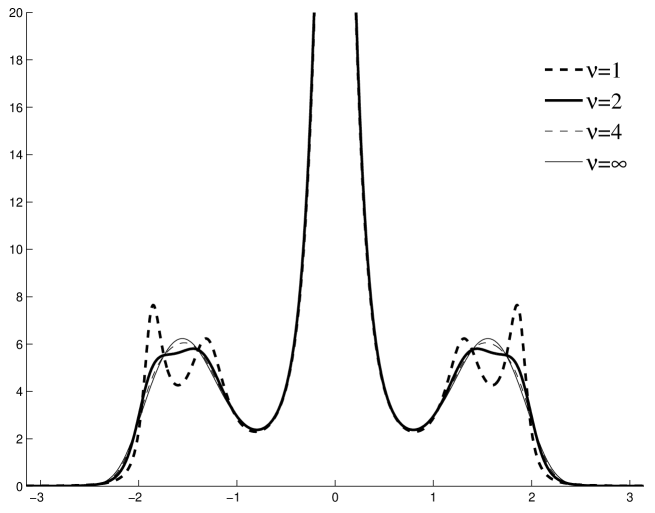
Figure 1: Approximations of $\Psi$ with different values of $\nu$.

In Figure 1 the approximations of $\Psi$ compatible with $\Sigma$ for $\nu=1$, $\nu=2$, $\nu=4$ and $\nu=\infty$ are depicted. It is clear that increasing $\nu$ the corresponding solution approaches the MinxEnt solution ($\nu=\infty$), and for $\nu=4$ it is pretty similar to the MinxEnt one. We have conducted other numerical experiments and we observed the same behaviour as $\nu$ increases.

8 Conclusion

We analyzed a spectrum approximation problem based on a suitable parametrization of the Alpha divergence family. Here, we make the mild assumption that the prior $\Psi$ is rational. When the parameter $\nu\in\mathbb{Z}$ is such that $1\leq\nu<\infty$, the corresponding family of solutions is rational with an upper bound on the degree equal to $\deg[\Psi]+2n\nu$. Moreover, the solution having the smallest upper bound is given by minimizing the Kullback-Leibler divergence with respect to the second argument (case $\nu=1$). Such solution also generalizes the approximation presented in [18] which only holds when the matrix $A$ is singular. When $\nu$ tends to infinity the solution of this family uniformly converges on $\mathbb{T}$ to an “exponential-type” solution having the same structure as the minimum discrimination information solution (MinxEnt) obtained with $\nu=\infty$. Moreover, numerical experiments show that solutions with $\nu$ large are almost equal to the MinxEnt solution. Hence, the family of solutions based on the Alpha divergence yields a concrete way to approximate the MinxEnt solution with a rational solution.