Recovery of fluctuation spectrum evolution from tomographic shear spectra

Abstract:

Forthcoming large angle surveys are planned to obtain high precision tomographic shear data. In principle, they will allow us to recover the spectra of matter density fluctuation, at various redshift, through the inversion of the expressions yielding shear from fluctuation spectra. This was discussed in previous work, where $SVD$ techniques for matrix inversion were also shown to be the optimal tool to this aim. Here we show the significant improvements obtainable by using a 7 bin tomography, as allowed by future Euclid data, and discuss error propagation from shear to fluctuation spectra. We find that the technique is a promising tool, namely for the analysis of baryon physics through high–$\ell$ shear spectra and to test the consistency between expansion rate and fluctuation growth.

1 Introduction

Dark Energy (DE) is one of the main discoveries – and puzzles – in contemporary physics. Cosmic Microwave Background spectra or Baryonic Acoustic Oscillations directly constrain its contribution to the cosmic budget, but only simultaneous low–$z$ measures of cosmic expansion rate and fluctuation growth can provide us real clues on DE nature [1]. In fact, besides of its state equation $w(z)$, we aim at knowing whether DE is a further physical dark component, or its observations are a signal of new physics, as GR violations [2], interactions between the dark components, possibly suggesting a unified picture for them [3, 4], or even more exotic scenarios [5, 6]. It is then worth outlining that, while SNIa data constrain the expansion rate, tomographic shear data enable us to follow the growth of density inhomegeneities. Being directly sensitive to the whole mass distribution, they also allow us to forget any problem related to light–mass conversion.

In order to exploit this kind of data, it has become customary to follow a Bayesian approach. We then consider a set of parameters spanning a wide set of models, for each of whom a number of observables can be predicted; predictions are then compared with observational data and relative errorbars, so obtaining likelihood hyper-elipsoïds in the parameter space. Similarly, when cosmic shear data will be available, one shall predict the tomographic shear spectra $C_{ij}(\ell)$ (the indeces $i,j$ run on the tomographic bins) and enrich the fit to data by comparing them with tomographic shear data.

In a previous paper ([7], Paper I herebelow) we considered a different option: directly deriving the spectra $P(k,z)$ at various redshift $z$ from $C_{ij}(\ell)$. A prediction of shear spectra is then no longer required, and shear data can soon be compared with other data on fluctuation growth, to be possibly used in parallel with them. To do so, we need to invert the integral relation yielding $C_{ij}(\ell)$ from $P(k,z)$. As we shall see, this option makes sense, in particular, if we wish to inspect background geometry and fluctuation dynamics separately.

In Paper I, our analysis was restricted to 5 tomographic bins. On the contrary, Euclid data, obtained from a celestial area of 15,000 square degrees with a median redshift $z_{m}=0.9$, will allow N–bin tomography, with N$\gg 5$ and up to 10 [8].

In this paper, we consider a 7 bin tomography and find that the improvements allowed by this N increase, when aiming to recover $P(k,z)$, are substantial. We shall also briefly comment on the reasons why attempting spectral recovery with $N>7$ leads to problems. The recovery still uses the singular value decomposition (SVD) technique for matrix inversion, an approach already followed by different authors in various physical contexts [9, 10]. Specific options of this technique, suitable to treat quasi–singular matrices, will be however used here for the first time in this context. Furthermore, we shall treat the question of noise propagation from shear to fluctuation spectra. Matrix theory allows us to predict upper limits to error magnification in such transition. Lukily enough, in this specific case, such limits are only marginally approached, while a simple filter allows us further noise reduction.

Let us also notice that, besides of verifying the coherence between expansion and fluctuation growths, this inversion technique could also facilitate the discrimination between different options on baryon physics, shaping $P(k,z)$ at high–$k$.

In order to test the inversion algorithm we need to input fluctuation spectra for a given model. We use them to build fluctuation spectra $P(k,z)$ at various redshifts and, from them, the shear spectra $C_{ij}(\ell)$. Successively, starting from $C_{ij}(\ell),$ we test how efficiently $P(k,z)$ is recovered. Being also interested in baryon physics and, therefore, having to explore the high–$\ell$ region, recent hydrodynamical simulations are used and briefly discussed. Let us however remind that the lensing spectra can be roughly shared in 3 $\ell$–ranges (see Figure 2, here below): The $C_{ij}(\ell)$ for $\ell<\sim 500$ essentially feel just the linear dynamics, even for $i,j=1$. For $500<\ell<1500$ the contribution coming from non–linear $k$’s becomes relevant. At $\ell>2000$, shear data start to exhibit a dependence on baryon physics.

The plan of the paper is as follows: In the next Section we shall review the procedure allowing to pass from data on galaxy ellipticity to shear spectra. In particular, we shall obtain the window functions in the 7–bin case, taking into account that, for most lensed galaxies, only photometric redshift will be avaiable.

In Section 3 fluctuation and shear spectra are defined and their relation set in an operational form. Section 4 debates the procedure of Gauss–Laguerre integration to obtain shear spectra from fluctuation spectra. Section 5 introduces the formal procedure to invert the equation yielding $C_{ij}(\ell)$ from $P(k,z)$, also based on Gauss–Laguerre integration. Section 6 then introduces the SVD technique and uses it for the study of the singularity level, as well to recover $P(k,z)$ from $C_{ij}(\ell)$, in 3 cases: (i) When $C_{ij}(\ell)$ is formally obtained with a GL integration technique. (ii) When $C_{ij}(\ell)$ is “exact”. (iii) When noise is added to it. Results are summarized and discussed in Section 7 and conclusions are drawn in Section 8, where we also outline possible options to improve the present approach.

2 Evaluation of shear–shear correlation functions

Using measured galaxy ellipticities [11, 12, 13] to gauge gravitational shear is a non–trivial task. Uncorrelated random ellipticities scarsely matter, the problem being intrinsic shear, due to nearby galaxy alignemnt. Assuming that data can reliably cleansed from it may be premature, but here we let apart this problem and proceed as though ellipticities due to gravitational shear only are measured (see however [14, 15, 16], and references therein).

We shall also assume (spatially flat) models whose background metric reads

$$ds^{2}=a^{2}(\tau)[d\tau-d\lambda^{2}]~{},$$ (1)

so that $\tau$ is the conformal time, $d\lambda$ being the comoving distance element, and $a(\tau)\equiv(1+z)^{-1}$ the scale factor. If $\tau_{0}$ is the present time,

$$u(z)=\tau_{0}-\tau(z)$$ (2)

is the conformal time distance –as well as the comoving distance– from $z$.

Let us also assume that galaxies observed in unit solid angle have a redshift distribution

$$n(z)={d^{2}N\over d\Omega\,dz}={\cal C}~{}\bigg{(}{z\over z_{0}}\bigg{)}^{A}\exp\bigg{[}-\left(z\over z_{0}\right)^{B}\bigg{]}$$ (3)

with $A=2$, $B=1.5$ so that

$${\cal C}={B/\left[z_{0}\Gamma\left(A+1\over B\right)\right]}={1.5/z_{0}}$$ (4)

(here $z_{0}=z_{m}/1.412$ while the median redshift $z_{m}=0.9~{}$, in agreement with Euclid specifications [8]). These phaenomenological values can be suitably modified, if needed.

To appreciate the effects of fluctuation evolution, galaxies are then shared into $N$ redshift bins, with limits $z_{r}$ selected so that they contain equal numbers of galaxies. For large galaxy sets, photometric redshifts only will be available and, to evaluate the expected distribution on redshift for the $r$–th bin galaxies, we can apply the filter

$$\Pi_{r}(z)=\int_{z_{r}}^{z_{r+1}}dz^{\prime}~{}{e^{-{(z-z^{\prime})^{2}\over 2\sigma^{2}(z)}}\over\sqrt{2\pi}~{}\sigma(z)}~{}=~{}{1\over 2}\left[{\rm Erf}\left(z_{r+1}-z\over\sqrt{2}\sigma(z)\right)-{\rm Erf}\left[z_{r}-z\over\sqrt{2}\sigma(z)\right]\right]$$ (5)

to $n(z)$, as suggested, e.g., in [17]. In this way we obtain the distribution

$$D_{r}(z)=n(z)\Pi_{r}(z)$$ (6)

whose integrals are $\simeq 1/N$, their sum being (exactly) $n(z)$. In this work we shall take $\sigma(z)=0.05~{}(1+z)$, coherently with Euclid expectations [8] (see also [18]).

Figure 1: l.h.s.: Total galaxy distribution $n(z)$ (red curve) and distributions $D_{r}(z)$ of the galaxies in $N=7$ bins as obtainable though photometric redshift values. Their sum (black dots) overlaps $n(z)$. r.h.s.: Window functions for the same 7 bin case.

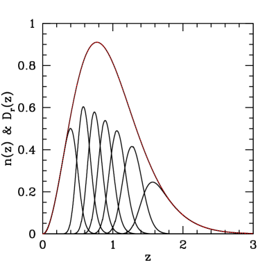
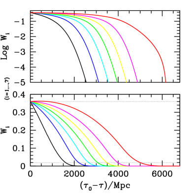
The images of galaxies belonging to a bin are lensed by the gravity of matter laying at lower $z$. This is taken into account by defining the window functions

$$W_{r}(z)={3\over 2}\Omega_{m}(1+z)\int_{\Delta z_{r}}dz^{\prime}~{}\delta_{r}(z^{\prime})~{}{\cal P}\left[u(z^{\prime})-u(z)\over u(z^{\prime})\right]~{};$$ (7)

here integration is restricted to the intervals $\Delta z_{r}$, where $D_{r}$ is non–zero, while

$$\delta_{r}(z)={D_{r}(z)/\int_{0}^{\infty}D_{r}(z^{\prime})dz^{\prime}}$$ (8)

and $\cal P$$(x)=x$ or 0 if $x>0$ or $<0$: only systems closer than a galaxy can distort its image. In Figure 1 we show $n(z)$ and $D(z)$ (l.h.s.), as well as $W_{r}(u)$ (r.h.s.), for the 7–bin case.

The cosmology used in this paper is the same of Paper I: a $\Lambda$CDM model with density parameters for matter and baryons, Hubble parameter, primordial spectral index and m.s. amplitude of density fluctuations, at $z=0$, on the scale of 8$\,h^{-1}$Mpc, shown herebelow

Table I

—————————————————————–

$$\matrix{\Omega_{m}&\Omega_{b}&h&n_{s}&\sigma_{8}\cr 0.24&4.13\times 10^{-2}&0.73&0.96&0.8}$$

—————————————————————–

To build the functions $W_{r}(z)$ we need to know $u(z)$. However, (i) no baryon physics is needed, not even the $\Omega_{b}$ value; (ii) fluctuation parameters, as $\sigma_{8}$ or $n_{s}$, are also not needed. This is to be borne in mind in view of the final discussion.

3 Density fluctuation and shear spectra

Figure 2: Integration patterns: red lines show $k$ values contributing to $C_{ij}(\ell)$ at given $\ell$ (aside them). At the r.h.s. of the cyan band, baryon physics yield significant contributions to spectra. Its slight (model dependent) decrease with $z$ is neglected here.

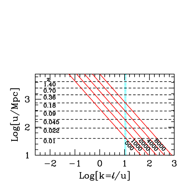
The shear–shear correlation functions $\xi_{+/-}^{ij}(\theta)$, derived from the distributions of the ellipticities of galaxies in the $i,j$–th bands, can be expanded in spherical harmonics yielding

$$\xi_{+/-}^{ij}(\theta)=(2\pi)^{-1}\int_{0}^{\infty}d\ell\,\ell\,J_{0/4}(\ell\theta)\,C_{ij}(\ell)$$ (9)

$J_{n}$ being first kind Bessel functions of order $n$. In turn, the shear spectra

$$C_{ij}(\ell)=H_{0}^{~{}4}\int_{0}^{\tau_{0}}du~{}W_{i}(u)W_{j}(u)~{}P[\ell/u,u]~{};$$ (10)

are related to the power spectrum $P(k,z)=\langle|\delta(k,z)|^{2}\rangle$; here $\delta(k,z)$ is the Fourier trasform of the density fluctuation field at redshift $z$. The functions $W_{i}(u)$ weight the contributions to shear correlations on the angular scale $\theta(\sim 2\pi/\ell)$, from density fluctuations over linear scales $\lambda(\sim 2\pi/k=2\pi u/\ell)$, increasing with $z$. Accordingly, shear correlations at a given $\ell$ receive contributions from decreasing $k$ values as $u$ increases. In turn, for $u\to 0$, $P(k,u)$ should be evaluated at $k\to\infty$ where, however, it vanishes. Figure 2 shows typical integration patterns on the $\log k$–$\log u$ plane, amounting to tilted straight lines.

4 Gauss–Laguerre integration procedure

Our aim now amounts to finding a technique to invert eq. (10) and to testing such technique; accordingly, eq. (10) is used first to work out the spectra $C_{ij}(\ell)$ for the given model. Then we test the algorithm –that we shall build– to reobtain $P(k,z)$ from $C_{ij}(\ell)$.

Fluctuation spectra at $k>\sim 10\,h$Mpc^-1 depend significantly on baryon physics. As substantial contributions to the integral (10) arise for $z>\sim 0.01$, Figure 2 shows that only $\ell\sim 500$ is (almost) free of baryon physics while, at $\ell>\sim 1500$, it becomes critical. Accordingly, to work out sensible $C_{ij}(\ell)$ spectra for $\ell>1500$, we need $P(k,z)$ obtained from hydro simulations. Analytical approximated expressions as Halofit are useful just for tests. In Appendix B we discuss the simulation used (the same as in Paper I) and interpolatory techniques. Here we assume $P(k,z)$ to be available at any $k$ and $z$ value.

Besides of performing the integral (10) with an “exact” adaptive Riemann integration, we need to consider a Gaussian integration procedure as well. It amounts to projecting each integrand function $f(u)=W_{i}(u)W_{j}(u)P(l/u,u)$ onto polynomials $\pi_{\alpha}(u)$, orthogonal with an assigned weight function $R$$(u)$, finding its components $f_{\alpha}$. As the integrals $\Pi_{\alpha}$ of each polynomial are known, $f(u)$ integral reads $\sum_{\alpha=1}^{\nu}f_{\alpha}\Pi_{\alpha}$. This is a reliable value if $\nu$ is large enough. This technique can be translated into a simple procedure, i.e. to a weighted sum of values taken by the integrand function $f(u)$ in a suitable set of points $u_{\alpha}$.

More in detail, by using monic polynomials (obtained from a recurrence relation assuming that the coefficient of the leading term, for each $\alpha$, is unity) we have that

$$\int_{0}^{\infty}dx\,\,R(x)\,\pi_{\alpha}(x)\pi_{\beta}(x)={\cal N}\delta_{\alpha\beta}\,\,,$$ (11)

with a known normalization $\cal N$. The $\nu$ zero’s of $\pi_{\nu}(x)$ are the points $x_{\alpha}$, while

$$w_{\alpha}={\int_{0}^{\infty}dx\,\,R(x)\pi_{\nu-1}^{2}(x)\over\pi_{\nu-1}(x_{\alpha})\pi^{\prime}_{\nu}(x_{\alpha})}\,\,\,,$$ (12)

are the corresponding weights ($\pi^{\prime}(x)$ being the ordinary derivative of $\pi(x)$). Accordingly

$$\int_{0}^{\infty}du\,f(u)=\int_{0}^{\infty}dx\,F(x)\,R(x)=\sum_{\alpha}w_{\alpha}F(x_{\alpha})~{}~{}~{}~{}{\rm with}~{}~{}~{}~{}F(x)={f[u(x)]\over R(x)}{du\over dx}~{}.$$ (13)

For $R(x)\propto e^{-x}$, the technique is dubbed Gauss–Laguerre (GL) integration, as $\pi_{\alpha}(x)=L_{\alpha}(x)$, the Laguerre polynomials. The integral (10) is cut off by the decay of the $W_{i}$ functions and GL integration can be applied by taking $x=(u/\bar{u})^{\beta}$, suitably selecting $\bar{u}$ and $\beta$.

Let us then rewrite eq. (10) as follows:

$$c_{A}(\ell)=\sum_{r=1}^{\nu}w_{r}S_{Ax_{r}}p_{x_{r}}(\ell)\equiv\sum_{r=1}^{\nu}{\cal M}_{Ar}p_{r}(\ell)\,\,\,~{}~{}{\rm being}~{}~{}c_{A}=C_{ij}/H_{0}^{4}~{},~{}~{}A\equiv ij$$ (14)

with

$$S_{Ax_{r}}=W_{i}(x_{r})W_{j}(x_{r})u_{r}/[\beta x_{r}R(x_{r})]\,,$$ (15)

$$p_{r}(\ell)\equiv p_{x_{r}}(\ell)=P_{\ell}(u_{r})=P(\ell/u_{r},u_{r})\,,$$ (16)

being $u_{r}=u(x_{r})$, and the correspondence law

$$\matrix{i,j&1,1&...&1,7&2,2&...&2,7&3,3&...&...&7,7\cr A&1&...&7&8&...&13&14&...&...&28}$$

5 Formal inversion

If, in eq. (14), we take $\nu=28$, ${\cal M}_{Ar}$ is a square matrix and, provided that it is non–singular, the inverse equation

$$p_{x_{r}}(\ell)=\sum_{A}({\cal M})^{-1}_{rA}c_{A}(\ell)$$ (17)

also holds. In principle, we should then be able to work out the spectrum $P(k,z)$ for any $k=\ell/u_{r}$, at the redshift values $z_{r}=z(u_{r})$. The inversion procedure acts on each $\ell$ value separately and we could even perform a different choice of $\bar{u}$ and $\beta$ for each $\ell$.

In Paper I, $\nu$ could reach atmost 15. This led to 2 difficulties: (i) 15 gaussian points could not allow us a nearly–exact integration; (ii) the determinant of the $15\times 15$ $\cal M$ matrix was close to singular. An inversion could however be achieved by passing from 15 to 12 integration point. Although worsening the (i) point, this allowed us a redundant system of equations, which could be treated through the SVD technique. A suitable choice of $\bar{x}$ and $\beta$ then allowed us to overcome the (ii) point and to approach an exact inversion of the $C_{ij}(\ell)$ spectra formally obtained through Gaussian integration.

However, even this was not enough when trying to invert the results of exact Riemann integration: the recovered $P(k,z)$ were systematically ill–normalized. Besides of the cosmological parameters needed to build the $W_{r}(u)$, we then needed to add $\Omega_{b}$ and $\sigma_{8}$ to predict the normalization (the dependence on $n_{s}$ is negligible). In this way we obtained all $P(k)$ details of at high–$k$ from $C_{ij}(\ell)$, but the linear $P(k,z)$ was assumed to be known.

Here we aim at testing whether 28 indipendent equations can do better. In particular, we aim at avoiding any input concerning baryonic and/or fluctuation parameters.

6 The SVD technique

The risk of singularity for the matrix

$${\cal M}_{Ar}=w_{r}W_{i(A)}(x_{r})W_{j(A)}(x_{r})u_{r}/[\beta x_{r}R(x_{r})]\$$ (18)

arises from the vanishing of low–$i$ window functions $W_{i}$, at distances $u_{r}$ (and thence at the corresponding $x_{r}$ values) where high–$i$ window functions are still significant.

The SVD technique, often used in science to handle complex datasets [9], here is used to evaluate, first of all, the degree of singularity of ${\cal M}_{Ar}$. The technique is based on a powerful theorem of linear algebra, stating that any real $N_{r}\otimes N_{c}$ matrix $\cal M$, with $N_{r}\geq N_{c}$, can be decomposed, in a unique way apart trivial overall factors, into a rows $\times$ columns product

$${\cal M}_{N_{r},N_{c}}={\cal U}_{N_{r},N_{c}}\times\left|~{}diag(s_{i})~{}\right|_{N_{c}}\times{\cal V}_{N_{c},N_{c}}^{T}$$ (19)

Here, in each index site, we set the range allowed to the index there. Both $\cal M$ and $\cal V$ ($\cal V$^T is its transposed) are orthonormal matrices; also $\left|~{}diag(s_{i})~{}\right|_{N_{c}}$ is a (fully diagonal) matrix.

If $N_{r}=N_{c}$, the inverse of $\cal M$, in general, reads

$${\cal M}^{-1}={\cal V}\times\left|~{}diag(1/s_{i})~{}\right|\times{\cal U}^{T}~{},$$ (20)

and the technique does not only invert large matrices, but also handles them when inversion is numerically hard. Fair manuals describing the SVD technique are [22, 23].

The $s_{i}$ components tell us the singularity level. When some of them vanishes, the matrix is singular and the problem is said to be ill–conditioned. Even if it is not so, as in our cases, the ratio between maximum and minimum $s_{i}$ (condition number) can exceed $\sim 10^{6}$ ($10^{12}$), and then there is no way to invert ${\cal M}$ in single (double) precision. Aiming at a precision $\cal O$$(1:10^{5}$–$10^{6})$, the top $s_{i}/s_{j}$ ratio must be within $\sim 10^{7}$. This is a necessary condition, however, not a sufficient one and we often need to be more restrictive.

6.1 Singularity level

Our first aim should amount to inverting the full 28² matrix. Its condition number depends on the choice of $\bar{u}$ and $\beta$. Best results are obtainable, as we discuss in Appendix B, when the top $z_{r}\sim 1.40$ and the low–$z$ domain is sampled at $z>\sim 0.02$ . In Figure 3 the Gaussian weights vs. the related redshift values and the components of the diagonal matrix $s$ are shown for $\bar{u}=351$, $\beta=1.8424$.

Figure 3: L.h.s.: Gauss–Laguerre weights vs. the related redshift values. R.h.s.: The elements $s_{i}$ of the diagonal matrix, yielding the singularity level of the matrix to be inverted.

Figure 4: GL and RI integration compared. The magnified frames at the l.h.s. outline residual oscillations in GL integrals.

Each $w_{r}$ is multiplied by $e^{x_{r}}$, so that also $w_{r}\sim 10^{-40}$ are not negligible. On the contrary, the $s_{i}$ components do span $\sim 13$ o.o.m. and inverting the $\cal M$ matrix, as it is, requires unusual computational resources.

The SVD approach however tells us how to deal with such a case, keeping as much information as possible. We can do so by simply setting to zero the unwanted $s_{i}$ values. For instance, once the last 7 (8) $s_{i}$ are zeroed, the residual $s_{i}$ just span 8 (7) orders of magnitude. This reduction, as explained in the cited manuals and discussed in Appendix B, is quite different from disregarding a number of equations: power spectra are recovered at all 28 redshifts and discrepancies from input spectra are safely small for $0.1\sim z\sim 1.2$. As a matter of fact, this is the very range where shear signals are reliable, and the matrix inversion technique substantially yields a best–fit recovery of input spectra.

Data on $C_{ij}(\ell)$ spectra will however come with errors and this is a critical point to apply this approach. To study their impact, we add a random Gaussian noise to the $C_{ij}(\ell)$ spectra worked out from $P(k,z)$. Inversion bursts the noise: an upper limit to noise magnification is set by the ratio between non–zero top and bottom $s_{i}$ (see Appendix B).

For instance, if such $s_{i}$ span 8 orders of magnitude, we are likely to obtain $C_{ij}(\ell)$ completely covered by noise. We therefore need to exploit the SVD technique at its limits, by keeping just a minimum number of non–zero $s_{i}$. Lukely enough, the transfered noise is then significantly below the theoretical upper limit and can be furtherly reduced by filtering.

In the next subsections we shall provide quantitative details on these points.

6.2 Recovery in the absence of noise

Two different integration technique have been considered here: (i) an adaptive Riemannian technique (RI, hereafter) allowing any wanted precision; (ii) a Gauss–Laguerre technique (GL, hereafter), that opens the door to inversion.

Although using 28 points and coefficients, GL does not allow us a full recovery of the $C_{ij}(\ell)$ obtained through RI. Although smoothed, simulation spectra keep some irregularities even for small $k$ increments. Even a 28–th degree polinomial is unable to follow all of them.

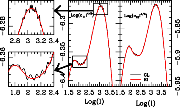
In Figure 4 we compare the results of GL and RI integration for $C_{11}(\ell)$ and $C_{22}(\ell)$ (the coefficient $H^{4}$ is omitted). The tiny differences ($\cal O$$.1\,\%$ at most) can be perceived, namely at low–$\ell$, where GL integrals exhibit tiny oscillations. When GL integration uses more usual numbers of points ($\sim 10$), these oscillations risk to be confused with BAO effects. A similar danger exhists if RI integration follows an interpolation of type (i), with not enough spectra along $z$. Spurious BAO’s are then an effect of the interpolating polinomials and disappear when we increase the number of spectra along $z~{}.$

In Figure 5 we show the results of matrix inversion if applied to GL spectra, using 20 or 21 $s_{i}$ values.

Figure 5: Recovery of $P(k,z)$ spectra, at the 5 redshifts shown in the frames, by using GL shear spectra and 21 (l.h.s.) or 20 (r.h.s.) non–zero $s_{i}$. Black (red) curves are the input (recovered) spectra. In the r.h.s. plot, recovery is so efficient that red lines mostly desappear below black ones.

Figure 6: As previous Figure, just using RI spectra and 16 (l.h.s.) or 15 (r.h.s.) non–zero $s_{i}$.

Figure 7: L.h.s.: As the previous Figure, just pushing the number of non–zero $s_{i}$ down to 6. R.h.s.: Inversion results, still with 6 non–zero $s_{i}$’s, after adding a noise $\simeq 0.8\,\%$. Mere inversion yields the cyan noisy curves. By applying a simple top–hat filter to them (average among 10 nearby $k$’s), errors are smoothed and we obtain the red curves.

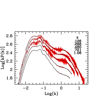
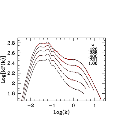
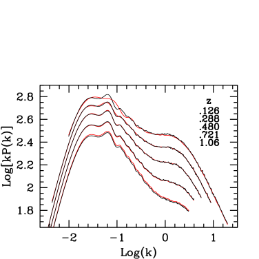
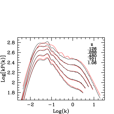
The passage from 8 to 7 o.o.m. in the $s_{i}$ selection is critical. In the 21–$s_{i}$ case, we see the low–$z$ spectra covered by the numerical noise. Notice also that the algorithm has however some difficulty to recover the BAO shape, namely at low $z$.

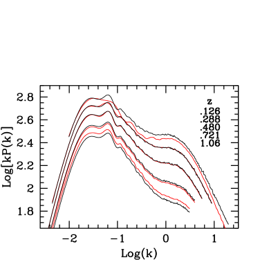
In Figure 5 and in the following ones we plot a selection of spectra, for the the same $z_{i}$ in all Figures, shown in the frame. In addition to the values plotted, there are $\sim 20$ intermediate $z_{i}$ values for which spectra are recovered with a precision similar to the best results shown.

We then apply the inversion algorithm, based on GL integration, on RI spectra. The transition from biased to fair spectra then occurs at the passage from 16 to 15 $s_{i}$ values. Unsatisfatory inversion is however appreciable here through curve confusion, rather than by curves obscured by numerical noise, as in Figure 5. The inversion is slightly less precise, typical errors being $\cal O$$(1\,\%)$, apart of the BAO range, where recovery appears more critical.

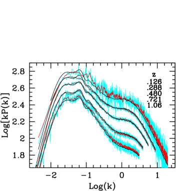
Before concluding the discussion on inversion in the absence of noise, let us consider also the option of keeping just 6 $s_{i}$ (Figure 7, l.h.s.). The efficiency of the SVD technique is so good that it still allows to recover a fair deal of spectra: in the $z$–range 0.2–1, $P(k,z)$ spectra are still recovered with errors $\cal O$$(2\,\%)$ for most of the $k$ range; BAO’s, however, tend to be badly recovered and spectra normalization are close to fair only for $0.2<z<1~{}.$

6.3 Recovery in the presence of noise

Error propagation from $C_{ij}(\ell)$ to $P(k,z)$ spectra is one of the contributions of this work. As above mentioned, in the process of matrix inversion errors expand. However, by suitably modeling available parameters, error increase can be kept under control. The cases shown here should be considered just as examples. Further improvement is still possible, e.g. by passing to a more efficient mapping from $u$ and $x$ variables. The noise in recovered $P(k,z)$ spectra is also filtered here in a simple fashion. More sophisticated filtering is possible.

We start then from RI $C_{ij}(\ell)$ spectra. By using a Gaussian random variable $G$, distributed around zero, whose variance is then set to $\epsilon$, we build the “noisy” spectrum

$$C^{(N)}_{ij}(\ell)=C_{ij}(\ell)\times[1+\varepsilon\,\,G]\,\,.$$ (21)

Cyan bands in Figure 7 (r.h.s.) show inversion results, obtained by keeping 6 non–zero $s_{i}$, with $\varepsilon=0.8\,\%$. Using 6 $s_{i}$’s yields a maximum/minimum $s_{i}$ ratio $\cal O$$(\sim 300)$ and this is also the theoretical upper limit to error magnification. Results are then filtered by using a 10–point top–hat filter (red curves). In the central $z$–range, after filtering errors are $\sim 5\,\%$, therefore keeping error magnification well within a factor $\sim 10\,.$

The point here is that reducing the maximum/minimum $s_{i}$ ratio has a twofold effect: it cuts off errors, but also kills the information in the $\cal M$ matrix. It may then be useful to consider the results shown in the Figures 8 in detail. The upper plots show the ratios between recovered and input $P(k,z)$ for 12 equispaced $z$ values, when SVD inversion is performed by using 7, 6 (and 5) non–zero $s_{i}$ and 10–point top–hat smoothing is performed. In each frame, the 3 colors yield 3 redshift values (shown aside). Each curve can be associated to its redshift by reminding that a $z$ increase shifts the $k$–range to the left.

We are also confident that more sophisticated filters could reduce errors by an extra factor $\sim 1/2$. If so, the expected error magnification factor $\sim 300$ could be curbed down to $\sim 3$.

Figure 8: Ratio between recovered and input power spectra at different redshifts (at the r.h.s. of top Figures), when the shear spectra is added a Gaussian noise $\sim 0.8\,\%$. The recovered spectra where filtered through a 10-point top–hat smoothing. These plots are obtained when 7 or 6 non–zero $s_{i}$ are kept. Reducing the number of non–zero $s_{i}$ reduces error magnification, but biases the inversion process. In the bottom Figure average displacements from unity of the ratios between input and recovered spectra are shown; errorbars yield m.s. oscillation amplitudes around average. Best results seem obtainable with 6 non–zero $s_{i}$.

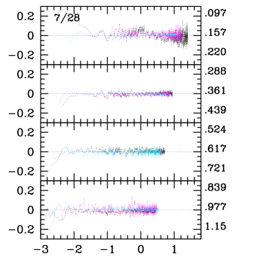
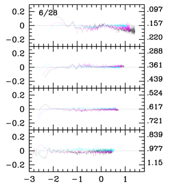
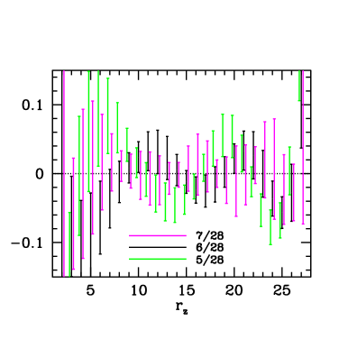
The bottom frame however shown that reducing the number of non–zero $s_{i}$’s yields a sort of oscillatory residuals, reminiscent of the use of a finite number of orthogonal polynomials. Reducing to 5 the number of non–zero $s_{i}$’s risks then to seriously bias the calibration of fluctuation growth through redshifts. Probably, to keep on the safe side, using 7 non–zero $s_{i}$ could be a fair choice. Testing advanced error filters with realistic error distributions, for the 7–$s_{i}$ case, could tell us a decisive word on the precision achievable.

7 Discussion

In this paper we discuss the invertion of the integral expression yielding tomographic shear spectra $C_{ij}(\ell)$ from density fluctuation spectra $P(k,z)$. In Paper I, the question had been discussed with (N=)5 bin tomography, yielding N(N+1)/2=15 independent shear spectra. We however expect future data (Euclid) to cover a larger sky portion, so allowing up to 10 bin tomography. Here, however, we considered just N=7, yielding N(N+1)/2=28 independent shear spectra, however allowing us great improvements in respect to N=5. Another contribution of this work is the study of noise propagation from tomographic shear data to fluctuation spectra.

We have started from the equation yielding shear from fluctuation spectra in the form

$$c_{A}={\cal M}_{A,r}p_{r}\,\,.$$ (22)

Here $C_{ij}(\ell)\equiv H^{4}c_{A}(\ell)$ and $p_{r}(\ell)=P(\ell/u_{r},u_{r})$, $u$ being the comoving distance of the redshift $z$. Eq.  (22) deals with each $\ell$ separately; summation replaces there integration and is performed by using a Gauss–Laguerre (GL) technique, by replacing the comoving distance $u$ by $x=(u/\bar{u})^{\beta}$ and assuming a large–$u$ behavior $\propto\exp(-x)$.

As $A$ takes 28 values, we are allowed a 28–point GL integration; the sum (22) then approaches the exact integral, even better. To obtain the matrix $\cal M$ we need information on the space geometry, as well as on the expected galaxy distribution on $z$ and the statistical relation between photometric and spectroscopic $z$’s.

Recovering $P(\ell/u_{r},u_{r})$ from $C_{ij}(\ell)$ then requires inverting the matrix $\cal M$. Unfortunately, as different bins refer to different depths, $\cal M$ approaches a singular behavior.

The recovery of $P(k,z)$ is therefore based on the singular value decomposition (SVD) technique, soon telling us the degree of singularity through the elements of a 28$\otimes$28 diagonal matrix $s$ derived from $\cal M$. The singularity however depends on the choice of $\bar{u}$ and $\beta$ and, in this work, we provide criteria for their selection. In spite of optimization, however, the $SVD$ approach tells us soon that the $s_{i}$ components span $\sim 13$ o.o.m.  (with the values adopted here, the maximum/minimum ratio is $\sim 1.22\times 10^{13}$). Let us also outline that passing to $N>7$ gives $\cal M$ matrices yielding $s_{i}$’s spanning even more o.o.m.’s.; e.g., for $N=8$ the $s_{i}$ elements span 18 o.o.m., at least.

The SVD technique however allows us to reduce the effective divergence level, by setting to zero a number of $s_{i}$. This is similar – but not equivalent and, indeed, not so drastic – to suppressing a number of equations. Our analysis exploits this option, also because error propagation depends on the ratio between minimum and maximum non–zero $s_{i}$.

The simplest task that the inversion procedure can accomplish is the recovery of $P(k,z)$ from $C_{ij}(\ell)$ obtainable via GL integration. The only limitation that we meet, in this case, is the divergence degree outlined by the diagonal $s$ matrix components. Out of 28 $s_{i}$ components, we find that best results are obtainable when keeping 20 non–zero $s_{i}$. Already with 21 components, numerical noise affects the low–$z$ recovered spectral components.

We then tested the inversion of the results of exact integration. Although being closer to realistic, this works as though adding a noise to the $c_{A}(\ell)$ components. As a matter of fact, to obtain fair results, we must then furtherly reduce the number of non–zero $s_{i}$. Best results are obtained with 15 $s_{i}$ components. Typical discrepancies between input and output fluctuation spectra are then $\cal O$$(2\,\%)$, apart of some wider discrepancy arising in the low–$k$ BAO range, namely for low redshift. Incidentally, this is a great improvement in respect to 5 bins. Then, the very normalization of recovered spectra was at risk and fair results could be obtained only through renormalization in the low–$k$ range.

We then tested error propagation by superimposing a Gaussian noise (m.s.a. $\sim 0.8\,\%$) onto the $C_{ij}(\ell)$ spectra obtained from the integration of simulation spectra. Noise is magnified by matrix inversion. A theoretical upper limit on noise magnification is set by the ratio between the top and bottom $s_{i}$ kept (see Appendix B). This calls for pushing further down the number of non–zero $s_{i}$. As a matter of fact, best results are obtained when keeping 6 or 7 non–zero $s_{i}$ (over 28!).

The noise in direct inversion results was then tentatively filtered by using a 10–point top–hat smoothing. After using this admittedly rough smoothing technique, we find that the overall noise magnification is less than a factor 10, in respect of a theoretical upper limit $\sim 300\,.$ Let us also outline that spectral values on nearby $k$ values derive from independent $\ell$ inputs, so that filtering acts in an “orthogonal” direction, in respect to matrix inversion.

The $k$–region most penalized by the suppression of a large number of $s_{i}$ is the BAO range. The first victim of the cut of $s_{i}$ is the possibility to recover the BAO structure.

Finally, let us briefly outline the problems arising with $N>7$, because of the greater range of o.o.m.’s spanned by the $s_{i}$ elements. With $N=7$ bands and in the most favorable case we have to suppress the matrix information related to 8 $s_{i}$, i.e. $\sim 30\,\%$ of it. Residual $s_{i}$ are within $\sim 7$ o.o.m.’s, allowing numerical routines $\sim 5$–6 o.o.m.’s, to work out reliable results.

In the same case, if $N=8$, to keep non–zero $s_{i}$ within 7 o.o.m.’s, one must give up almost half of them. Spectral recovery still works, but errors are wider. The problem is clearly in numerical precision. Using quadruple precision in not trivial, but possible, and would allow us to exploit $N>7$ bands.

8 Conclusions

Shear data are expected to be a new and effective resource to discriminate among cosmological models. They are most sensitive to the rate of expansion and fluctuation growth at low–$z$, when the contribution of Dark Energy is determinant. Accordingly, they are expected to be an outstanding probe on the DE equation of state $w(z)$ and on possible deviation from GR, or to couplings between the dark cosmic components.

From data we expect tomographic shear spectra to be derived. A basic difficulty amounts to cleansing rough data from intrinsic ellipticities. Here we assume that this aim has been achieved and that we can use any number of bins up to 10.

An analysis of spectral data can be performed in accordance with a Bayesian paradigm: $C_{ij}(\ell)$ model predictions are then made and compared with $C_{ij}(\ell)$ data and their errorbars.

Other datasets, also from the same Euclid experiment, will directly concern $P(k,z)$ spectra. The option to skip $C_{ij}(\ell)$ model predictions, by directly associating $P(k,z)$ spectra derived from them with other $P(k,z)$ data, is then appealing. By using double precision routines, best results are obtainable if $C_{ij}(\ell)$ come from 7 bins. A rather satisfactory test on error magnification in this derivation has also been performed here, but it is perhaps premature to state that errors are under control. This seems the main point to be further deepened in future work.

To build the $\cal M$ matrix, whose inversion allows us to work out $P(k,z)$ from $C_{ij}(\ell)$, we need to convert redshifts into distances. Model geometry must then be known, but neither $\sigma_{8}\,\,$ and $n_{s}$, nor parameters describing baryon physics (including $\Omega_{b}$) shall be input.

For the sake of example, let us then outline a possible investigation pattern: SNIa data could become so good that the distance modulus could provide $u(z)$ with negligible errors. From such $u(z)$ the parameters of background cosmology can be derived. However, independently from such derivation, we can use $u(z)$ to build the window functions $W_{r}(u)$ and derive from them the inverted matrix ${\cal M}^{-1}$, so obtaining $P(k,z)$ – apart of a constant factor $(\Omega_{m}H_{0}^{2})^{2}\,$– and the growth law $G(a)$. In parallel with fitting $u(z)$ to models, we then also fit $G(a)$ to them, so performing two independent model tests, based on geometry and dynamics, respectively. The two tests could provide a direct confirm/falsification of models where DE and DM are two real and independent cosmic components.

More in general, this technique allows us to measure the fluctuation growth in an unbiased way, over any $k$–range, namely those where different hypotheses on stellar formation, SN explosion, AGN energy release, etc., are critical. Accordingly, the inversion technique might become an important tool to discriminate among different hypotheses on baryon physics, possibly testing parameters beyond those spanning the bayesian parameter space.

Let us then outline that there is still room for further improvements of the technique providing $P(k,z)$ from shear spectra. In particular, let us stress the following points: (i) A great improvement was achieved when passing from N=5 to N=7; further improvements may be at hand if using 8, 9, or 10 bins. This just requires going beyond double precision. (ii) Noise propagation was considered here to test error propagation. Propagated noise was then filtered, with an effective but rought procedure. Better filtering techniques are surely available, but selecting among them depends on the nature of the “noise” used to describe errors. (iii) A technical issue concerns the passage from the coordinate $u$ to the integration variable $x$. The choise of $\bar{u}$ and $\beta$ in the conversion expression $x=(u/\bar{u})^{\beta}$ was found to be critical. No $u$–$x$ mapping more evolute than a simple power low was however considered; their use in the low–$x$ range could allow us further improvements.

Since a few decades, various authors devoted their efforts to invert the Limber equation [25], aiming at obtaining the spatial correlation function from the angular one, without making an ansatz on its shape. Nice algorithms were built, also taking into account relativistic effects [26, 27, 10]. Unfortunately, none such algorithm really found a practical application to data analysis.

Also the equations inverted here are a sort of Limber equation, but one should avoid to infer, from past failures, that this approach will face unsurmontable practical difficulties, as well. Of course, lensing angular spectra, instead of angular positions, are used here and, in a sense, this makes the problem harder. However, tomographic data are used here: a third coordinate is therefore input and the whole technique makes an extensive use of it.

ACKNOWLEDGMENTS. SAB acknowledges the support of CIFS. We are grateful to Stefano Borgani for making available to us his large hydrodynamical simulations and to Volker Springel for the non-public GADGET-3 code used to run them. Giuseppe La Vacca is also gratefully thanked for a number of useful discussions. H. Hoekstra, T. Kitching, L. Guzzo and W. Percival are also to be thanked for comments.

Appendix A

1. A brief description of the simulation used

The simulation box side $L=410\,h^{-1}$Mpc ($k_{L}=2\pi/L\sim 1.5\times 10^{-2}\,h\,$Mpc^-1); $(2\times)1024^{3}$ particles are used, with a force resolution $\epsilon=7.5\,h^{-1}$ kpc ($k_{\epsilon}=2\pi/\epsilon\sim 8.4\times 10^{2}\,h$Mpc^-1). Spectra can be used up to $k\simeq N(2\pi/L)$ with $N\simeq 2^{15}=32768$, however keeping $k~{}(\simeq 5.0\times 10^{2}\,h$Mpc${}^{-1})<k_{\epsilon}$, provided that they are not covered by shot noise (see [19]).

According to Table I of Section 2, CDM and baryon particle masses are $m_{c}\simeq 1.89\times 10^{9}\,h^{-1}M_{\odot}$ and $m_{b}\simeq 3.93\times 10^{8}\,h^{-1}M_{\odot}$, respectively. Baryon dynamics includes cooling and star formation. Metal production from chemical enrichment contributed by SN-II, SN-Ia and AGB stars, as described in [20], is also included. Stars, distributed according to a Salpeter IMF, release metals over the time-scale determined by the corresponding mass-dependent life-times. Kinetic feedback is also implemented by mimicking galactic ejecta powered by SN explosions. AGN feedback is not included, at variance from [21], who however used smaller boxes. The simulation start at $z=41$ and spectra are obtained at

$$1+z_{r}=10^{r/20}\,\,\,\,\,\,\,(r=1,\,....\,,19)\,\,.$$ (23)

8 of them, up to $z\simeq 1.24$ are between 0 and 1.4; 7 more are within $z=4.02$. For more details see [19]. These 15 spectra are used for interpolation.

2. Spectra interpolation

There are at least 3 different patterns to interpolate, schematically shown in Figure 9.

Figure 9: Interpolation patterns. In the Figure we assume “data” to be available at the crossings between horizontal and vertical dotted lines. The tilted lines are at constant $\ell$. Along one of them, we indicate a typical set of points where we may need to know $P(l/u,u)$, to perform the numerical integration. To reach them, in any case, there are 2 interpolation steps. The direction of former (latter) is indicated by the two parallel segments (a single segment, tilted or orthogonal).

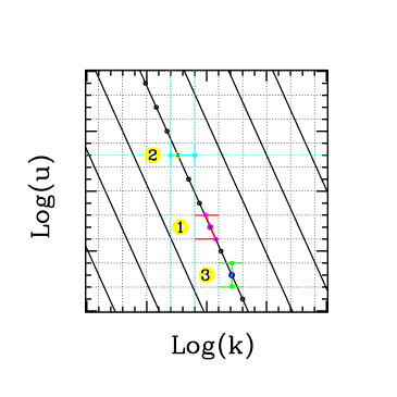
(1) We can first work out $P_{\ell}(u_{a})\equiv P(\ell/u_{\alpha},u_{\alpha})$ at fixed $\ell$, by interpolating among $k_{b}$ values. To perform the integral we need $P_{\ell}(u)$ at suitable values of $u\neq u_{a}$, and this requires a further interpolation at constant $\ell$. (2) We can first determine $P(k_{b},u)$ at the $u$ value needed; then interpolate at constant $u$ along $k$. (3) We can first determine $P(k,u_{a})$ at the $k$ value needed; then we interpolate at constant $k$ along $u$.

Interpolation involves more than the 2 closest points in each direction. Thick segments connecting 2 close points are just as an indication of the directions along which one uses a cubic spline.

By using the Halofit algorithm, yielding spectra at arbitrary $k$ and $u$ we found that the procedures (2) & (3) perform similarly. On the contrary, the procedure (1) (interpolation along tilted $\ell$–constant curves) yields consistent results only when spectra are known at $\sim 3$ times more redshift values $z_{a}$. Still using HALOFIT we tested that our simulation “data” is adequate for procedures (2) and (3), as far as $k$ and $z$ values available.

Appendix B

1. The singular value decomposition (SVD)

The SVD technique is based on a theorem of linear algebra stating that any $M\times N$ ($M>N$) matrix $\cal M$ can be decomposed, in a unique way apart of multiplicative factors, into the matrix product $U\cdot s\cdot V^{T}$ ($V^{T}$ is the transpose of a matrix $V$). More in detail:

$$\left|\matrix{{\cal M}_{11}&...&{\cal M}_{N1}\cr....&...&....\cr{\cal M}_{1M}&...&{\cal M}_{NM}}\right|=\left|\matrix{U_{11}&...&U_{N1}\cr....&...&....\cr U_{M1}&...&U_{NM}}\right|\cdot\left|\matrix{s_{1}&0&0\cr...&...&...\cr 0&0&s_{N}}\right|\cdot\left|\matrix{V^{T}_{11}&...&V^{T}_{N1}\cr....&...&....\cr V^{T}_{N1}&...&V^{T}_{NN}}\right|~{},$$

with a diagonal $s$, while $U$ and $V$ are orthogonal, i.e.,

$$\sum_{i}U_{ia}U_{ib}=\delta_{ab}~{},~{}~{}~{}\sum_{i}V_{ia}V_{ib}=\delta_{ab}~{},$$

or

$$U^{T}\cdot U={\mathbf{1}}~{},~{}~{}~{}V^{T}\cdot V={\mathbf{1}}~{}.$$

In this work we are interested just in the case when $M=N$ and all matrices are square; accordingly, it is also $U\cdot U^{T}={\mathbf{1}}$ (and $V\cdot V^{T}={\mathbf{1}})$. The condition number of the matrix $\cal M$ is then defined as the ratio $K$ between the largest and smallest (in magnitude) $s_{i}$. A matrix is said to be ill–conditioned if $K$ is too large (or singular if $K\to\infty$).

2. Norms and error magnification

Let us recall first that the (2–)norm of a vector x reads

$$|{\bf x}|=\left[\sum_{i}|x_{i}|^{2}\right]^{1/2}$$

$x_{i}$ being its components. The (2–)norm of a matrix A is then defined as follows:

$$|{\bf A}|=max\left(|{\bf A\cdot x}|\over|{\bf x}|\right)$$

i.e.: $|{\bf A}|$ is the maximum factor by which the matrix A can amplify a non–zero vector x. It can then be shown that, if we perform a SVD of A and $s_{1}$ is the top component of the diagonal matrix ${\bf s}$, in the relation ${\bf A}={\bf U}\cdot{\bf s}\cdot{\bf V}^{-1}~{},$ it is

$$|{\bf A}|=s_{1}~{}.$$

Let us then outline that, if we state $t_{i}=s_{i}^{-1}$, it is ${\bf A}^{-1}={\bf V}\cdot{\bf t}\cdot{\bf U}^{-1}~{}.$ Accordingly, $|{\bf A}^{-1}|=1/s_{n}~{},$ $s_{n}$ being the smallest component of the matrix ${\bf s}$ and

$$|{\bf A}|\cdot|{\bf A}^{-1}|=s_{1}/s_{n}~{}.$$

The matrix–vector and matrix–matrix products have then the following properties:

$$|{\bf A\cdot x}|\leq|{\bf A}|\cdot|{\bf x}|~{}~{}~{}~{}{\rm and}~{}~{}~{}~{}|{\bf A\cdot B}|\leq|{\bf A}|\cdot|{\bf B}|~{}.$$

Let us then assume that

$${\bf A}\cdot{\bf x}={\bf b}$$

and consider $\tilde{\bf x}={\bf x}+\delta{\bf x}$, as we do when we try to reobtain $P(k,z)$ from noisy $C_{ij}(\ell)$. It shall be ${\bf A}\cdot\tilde{\bf x}={\bf b}+\delta{\bf b}$ and therefore $\tilde{\bf x}-{\bf x}={\bf A}^{-1}\cdot\delta{\bf b}~{},$ so that, owing to eq. (B6), $|\delta{\bf x}|\leq|{\bf A}^{-1}|\cdot|\delta{\bf b}|~{}.$ In turn, eq. (B7) yields

$${1\over|{\bf x}|}\leq{|{\bf A}|\over|{\bf b}|}~{}~{}~{}~{}{\rm and,~{}therefore}~{}~{}~{}~{}{|\delta{\bf x}|\over|{\bf x}|}\leq|{\bf A}|\cdot|{\bf A}^{-1}|\cdot{|\delta{\bf b}|\over|{\bf b}|}~{}.$$

Owing to eq. (B5) we have then that

$${|\delta{\bf x}|\over|{\bf x}|}\leq{s_{1}\over s_{n}}\cdot{|\delta{\bf b}|\over|{\bf b}|}~{}.$$

i.e., that error magnification is surely smaller than the ratio between the maximum and minimum $s$ components considered, coinciding with the condition number $K$.

For the proofs of the theorems, besides of [22, 23], see also [24].

3. Gauss–Laguerre parameter selection

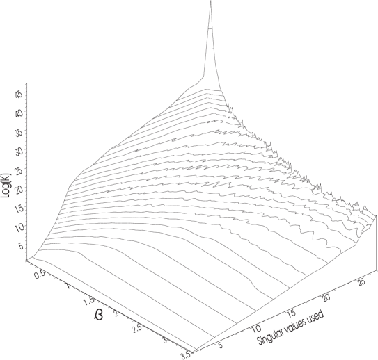
The Gauss–Laguerre sum, replacing the integration over $P(k,z)$ to obtain the shear spectra $C_{ij}(\ell)$, ought to by made with an eye to the matrix inversion which will follow. The condition number $K$ of the matrix $\cal M$, in fact, depends in a critical way on the selection of the $\bar{u}$ and $\beta$ parameters used in the change of variable $x=(u/\bar{u})^{\beta}~{}.$ A bad selection of $\bar{u}$ and $\beta$ can yield $K$ values up to $10^{20}$ or even larger. Moreover, $K$ is also directly linked to error magnification, according to eq. (B7).

To minimize $K$ we can act on 3 parameters: $\beta$, $\bar{u}$, and $N_{cut}$, the number of $s_{i}$ which (unavoidably) will be set to zero. Increasing $N_{cut}$ obviously reduces $K$, but our aim amounts to minimizing $K$ while keeping $N_{cut}$ sufficiently low, so to grant a fair and physical solutions to the a substantial part of the 28 equations forming the linear system.

Let us then keep into account that the galaxy redshift distribution $n(z)$ rapidly declines beyond $z\sim 1$ and that, therefore, the window functions $W_{r}$ and the $\cal M$ matrix element also fade. In the following we shall not directly consider contributions coming from above a maximum redshift $z_{max}=1.4$, corresponding to a maximum comoving distance $u_{max}=4194\,$Mpc, a choice yielding fair results. We shall then select the value of $\bar{u}$ so that

$$\bar{u}(\beta)={u_{max}}/{x_{M}^{1/\beta}}$$

$x_{M}$ being the largest node in the Gauss-Laguerre integration.

With this rule, we can then estimate the condition number for a wide range of $\beta$ (from $0.1$ to $3.5$) and $N_{cut}$ values. The latter parameter will be considered in the interval 0 (all singular values kept) –26 (only the two largest singular values kept, to estimate their ratio).

In Figure 10, $K$ is plotted as a function of $\beta$ and of the residual $s_{i}$ number ($28-N_{cut}$). The plot shows how dramatically $K$ blows up just by choosing unsuitable values of the free parameters. It is also evident that, reducing the number of non–zero $s_{i}$, $K$ sistematically decreases and that, for a given number of non–zero $s_{i}$, $K$ depends on $\beta$.

However, when the number of non-zero $s_{i}$ is small ($<\sim 10$) the $K$ dependence on $\beta$ weakens. This can be exploited to perform slight changes of the $\beta$ value, yielding a suitably different set of $u_{r}$ for the Gauss–Laguerre nodes $x_{r}$. In this way, we can obtain $P(k)$ at almost any $z$ value, in the $z$–range where matrix inversion is efficient (see text).

Figure 10: The condition number $K$ vs. the number of non–zero $s_{i}$ kept and $\beta$. At high $K$, there appear some graphic irregularities in the curves, due to the discreteness of the $s_{i}$ number.

References

- [1] Albrecht A. et al. 2006, “Report of the Dark Energy Task Force”, APS meeting abstract, APR, G1002; also: arXiv:astro-ph/0609591
- [2] S. Capozziello, S. Nojiri, S. D. Odintsov and A. Troisi, Phys. Lett. B 639 (2006) 135; L. Amendola, D. Polarski, and S. Tsujikawa, Are f(R) dark energy models cosmologically viable? Phys. Rev. Lett. 98 (2007), 131302; L. Amendola, R. Gannouji, D. Polarski and S. Tsujikawa, Phys. Rev. D 75 (2007) 083504; P. Creminelli, G. D’Amico, J. Norena, & F. Vernizzi, The Effective Theory of Quintessence: the Side Unveiled, J. of Cosm. & Astrop. Phys. 0902 (2009) 018; M. Park, K. M. Zurek, and S. Watson, A Unified Approach to Cosmic Acceleration, Phys. Rev. D 81 (2010) 124008; J. K. Bloomfield and E. E. Flanagan, A Class of Effective Field Theory Models of Cosmic Acceleration, J. of Cosm. & Astrop. Phys. 10 (2012) 039
- [3] T. Damour, Gibbons G. W., Gundlach C., Phys.Rev.Lett. 64 (1990) 123 ; C. Wetterich , A&A, 301 (1995) 321; Amendola L. Phys.Rev.D 62 (2000) 643511; Amendola L., Quercellini C., Phys Rev D68 (2001) 023514; Amendola L., Tocchi Valentini D. Phys. Rev. D66 (2002) 041528; Andrea V. Maccio’, Claudia Quercellini, Roberto Mainini, Luca Amendola, Silvio A. Bonometto, N-body simulations for coupled dark energy: halo mass function and density profiles, Phys.Rev.D69 (2004) 123516; Roberto Mainini, Silvio A. Bonometto, Dark Matter and Dark Energy from the solution of the strong CP problem, Phys.Rev.Lett. 93 (2004) 121301; Mainini Roberto, Silvio Bonometto, Dark Matter & Dark Energy from a single scalar field: CMB spectrum and matter transfer function, JCAP 0709 (2007) 017; L.P.L. Colombo, R. Mainini, S. A. Bonometto, Do WMAP data favor neutrino mass and a coupling between Cold Dark Matter and Dark Energy?; J. R. Kristiansen, G. La Vacca, L. P. L. Colombo, R. Mainini, S. A. Bonometto, Coupling between cold dark matter and dark energy from neutrino mass experiments, New Astron.15 (2010) 609; W. Zimdahl, D. Pavon, and L. P. Chimento, Interacting quintessence, Phys. Lett. B 521 (2001), 133; S. del Campo, R. Herrera, G. Olivares, and D. Pavon, Interacting models of soft coincidence, Phys. Rev. D 74 (2006), 023501; L. Amendola, G. C. Campos, and R. Rosenfeld, Consequences of dark matter-dark energy interaction on cosmological parameters derived from SN Ia data, Phys. Rev. D 75 (2007), 083506; Z. K. Guo, N. Ohta, and S. Tsujikawa, Probing the coupling between dark components of the universe, Phys. Rev. D 76 (2007), 023508; G. Caldera-Cabral, R. Maartens, and L. A. Urena-Lopez, Dynamics of interacting dark energy, Phys. Rev. D 79 (2009), 063518; Valeria Pettorino, Luca Amendola, Carlo Baccigalupi, Claudia Quercellini, Constraints on coupled dark energy using CMB data from WMAP and SPT, arXiv:1207.3293
- [4] M.C. Bento, O. Bertolami, Dark energy and the Rutherford-Soddy radiative decay law Phys.Lett.B675 (2009) 231; M.C. Bento, R. Gonzalez Felipe, The variation of the electromagnetic coupling and quintessence, Phys.Lett.B674 (2009) 146-151; M.C. Bento, R. Gonzalez Felipe, N.M.C. Santos Brane assisted quintessential inflation with transient acceleration , Phys.Rev. D77 (2008) 123512
- [5] K. Tomita, Distances and lensing in cosmological void models, Astrophys. J. 529 (2000), 38; M. N. Celerier, Do we really see a cosmological constant in the supernovae data?, A & A 353 (2000) 63; K. Tomita, A local void and the accelerating universe, Mon. Not. Roy. Astron. Soc. 326 (2001), 287; H. Iguchi, T. Nakamura, and K. i. Nakao, Is dark energy the only solution to the apparent acceleration of the present universe?, Prog. Theor. Phys. 108 (2002), 809; R. Jimenez, P. Talavera, & L. Verde, An effective theory of accelerated expansion, arXiv:1107.2542
- [6] T. Buchert, Dark energy from structure – A status report, Gen. Rel. Grav. 40 (2008) 467; S. Rasanen, Dark energy from backreaction JCAP 0402 (2004) 003; E. W. Kolb, S. Matarrese, A. Notari, and A. Riotto, The effect of inhomogeneities on the expansion rate of the universe, Phys. Rev. D 71 (2005) 023524; E. W. Kolb, S. Matarrese, and A. Riotto, On cosmic acceleration without dark energy, New J. Phys. 8 (2006) 322; C. M. Hirata and U. Seljak, Can superhorizon cosmological perturbations explain the acceleration of the universe?, Phys. Rev. D 72 (2005), 083501; P. Martineau and R. H. Brandenberger, The effects of gravitational back-reaction on cosmological perturbations, Phys. Rev. D 72 (2005) 023507; A. Ishibashi and R. M. Wald, Can the acceleration of our universe be explained by the effects of inhomogeneities?, Class. Quant. Grav. 23 (2006), 235; M. Kasai, H. Asada, and T. Futamase Toward a no-go theorem for accelerating universe by non-linear backreaction, Prog. Theor. Phys. 115 (2006) 827; S. Rasanen, The effect of structure formation on the expansion of the universe, Int. J. Mod. Phys. D 17 (2009) 2543; F. Piazza, Modifying gravity in the infra-red by imposing an ‘ultra-strong’ equivalence principle, arXiv:hep-th/0904.4299 (2009); F. Piazza, The IR-completion of gravity: What happens at Hubble scales?, New J. Phys. 11 (2009) 113050; V. Silveira & I. Waga, Decaying Lambda cosmologies and power spectrum, Phys. Rev. D 50 (1994) 4890
- [7] Mezzetti Marino, Bonometto Silvio A., Casarini Luciano & Murante Giuseppe, Direct recovery of fluctuation spectra from tomographic shear spectra, JCAP.06 (2012) 005 (Paper I)
- [8] Laureijs R. et al., 2012, SPIE Proceedings 8442, 32; Refregier A., Amara A., Kitching T. D., Rassat A., Scaramella R., Weller J., et al. 2010, [arXiv:1001.0061]
- [9] Donaher S., Fegam D.J. & Hagan J., 1993, Application of SVD in high–energy –ray astronomy, Astropart. P. 1, 357; Hurrel J.W., 1995, Decadal trends in the North Atlantic oscillations: Regional Temperature & Precipitation, Science 269, 676; Rucinski S., 1999, Precise Stellar Radial Velocities, IAU Colloquium 170. Eds. J.B. Hearnshaw and C.D. Scarfe. ASP Conference Series n. 185, 82 & astro–ph/9807327
- [10] Eisenstein D.J. & Zaldarriaga M., 2000, Correlations in Spatial Power Spectrum Inferred from Angular Clustering: Methods & Applications to APM, AAS Bull. 32, 684 & astro–ph/9912149
- [11] Kamionkowski M., Kosowhy B. & Stebbins A., Phys. Rev. D55 (1997) 7368
- [12] Crittenden R.G., Natarajan P., Pen U. & Theuns T. , Spin-induced Galaxy Alignments and Their Implications for Weak-Lensing Measurements, ApJ 559 (2001) 552; Huterer D., 2002, Phys. Rev. D 65, 063001; Huterer D. and Takada M., 2005, Astropart. Phys. 23, 369.
- [13] Stebbins A., Weak Lensing On the Celestial Sphere, astro-ph/9609149
- [14] Bridle S.L. & King L., Dark Energy constraints from shear power spectra: impact of intrinsic alignements on photometric redshift requirements, 2007, NJPh 9, 444
- [15] Schrabback T. et al., Evidence of accelerated expansion of the Universe from weak lensing tomography with COSMOS, A&A 516 (2010) 63
- [16] Joachimi B. & Bridle S.L., Simultaneous measurement of cosmology and intrinsic alignments using joint cosmic shear and galaxy number density correlations, 2010, A&A 523, A1
- [17] Hu, W., 1999, Astrophys. J. 522, L21; Hu W., Ma Z. and Huterer D., 2006, Astrophys. J. 636, 21; Bernstein G. and Ma Z., 2008, Astrophys. J. 682, 39; Casarini L., La Vacca G,, Amendola L., Bonometto S.A., Macciò A.V., 2011, JCAP03, 026
- [18] Amara A. & Refrégier A., 2007, MNRAS 381, 1018; Amendola L., Kunz M. & Sapone D., JCAP 0804 (2008) 013
- [19] Casarini L., Bonometto S. A., Borgani S., Dolag K., Murante G., Mezzetti M., Tornatore L., La Vacca G., Tomographic weak-lensing shear spectra from large N-body and hydrodynamical simulations, A&A 542 (2012) 126
- [20] Tornatore L., Borgani S., Dolag K. & Matteucci F., Chemical enrichment of galaxy clusters from hydrodynamical simulations, MNRAS 382 (2007) 1050
- [21] Semboloni E., Hoekstra H., Schaye J., van Daalen M.P., McCarthy I.G., 2011, arXiv:1105.1075; Quantifying the effects of baryonic physics on weak lensing tomography, MNRAS 417 (2012) 2020; see also: Semboloni E., Hoekstra H., Schaye J., arXiv:1210.7303 Effects of baryonic feedback on two and three point shear statistics: prospects for detection and improved modeling.
- [22] Press W.H., Teukolsky S.A., Vetterling W.T. & Flannery B.P., 1992, Numerical Recipes, Cambridge Univ. Press, par. 2.6 .
- [23] Golub G.H. & Van Loan C.F., 1989, Matrix Computations, J.Hopkins Univ. Press, par. 5.2.6 .
- [24] G.M. Phillips & P.J. Taylor, Theory and Applications of Numerical Analysis, Academic Press, Edition, 1996; L.N. Trefethen & D. Bau III, Numerical Linear Algebra, Society for Industrial and Applied Mathematics (SIAM), Philadelphia, 1997
- [25] Limber, D.N. 1953, ApJ, 117, 134
- [26] Groth E.J. & Peebles P.J.E., 1977, ApJ, 217, 592; Phillips S., Fong R., Ellis R.S., Fall S.M., MacGillivray H.T. 1978, MNRAS 182, 673
- [27] Bonometto S.A. & Lucchin F., 1978, Inversion of Limber’s Relativistic Formula, A&A 67, 153