Hadronic Screening in Improved Taste
Abstract
We present our results on meson and nucleon screening masses in finite temperature two flavour QCD using smeared staggered valence quarks and staggered thin-link sea quarks with different lattice spacings and quark masses. We investigate optimization of smearing by observing its effects on the infrared (IR) and ultraviolet (UV) components of gluon and quark fields. The application of smearing to screening at finite temperature also provides a transparent window into the mechanism of the interplay of smearing and chiral symmetry. The improved hadronic operators show that above the finite temperature cross over, , screening masses are consistent with weak-coupling predictions. There is also evidence for a rapid opening up of a spectral gap of the Dirac operator immediately above .
pacs:
12.38.Mh, 11.15.Ha, 12.38.GcI Introduction
Screening masses control finite volume effects at finite temperature in equilibrium. Studies of the final state of fireballs produced in heavy-ion collisions indicate that they are near equilibrium. So the study of screening masses a little below the QCD cross over temperature, near the freeze out, should improve our understanding of experimental conditions. In addition, the vector screening masses below should be of direct relevance to the study of mass spectra of dileptons and photons.
There are also interesting questions about the nature of the high temperature phase which are addressed by a study of screening masses. In QCD at temperatures, , of a few times the crossover temperature, , analysis of the weak coupling series in powers of the gauge coupling, , indicates that the physics of the magnetic scale of momentum, , is potentially non-perturbative. As a result, it may be possible to find phenomena in hot QCD, only involving harder scales, which are amenable to a suitable weak coupling analysis. For example, the fermionic part of the pressure, as well as its derivatives with respect to chemical potentials, the quark number susceptibilities (QNS), seem to admit reasonably accurate weak-coupling descriptions at temperatures of or above qcdft .
However, even among static fermionic quantities, screening masses (the inverses of screening lengths) present a confused picture. Most computations have been performed with staggered quarks, and these seem to indicate that there are strong deviations from weak coupling prediction kogut ; fftmass ; quasi ; cheng ; edwin . On the other hand, computations with Wilson quarks give results which are closer to free field theory brandt , although they deviate in detail from predictions of weak coupling theory dr ; htl . Since the same pattern is visible in the quenched theory scrnp , we can attribute the major part of the discrepancy to valence quark artifacts. Here we examine this question systematically using staggered sea quarks and improved staggered valence quarks. Indeed, we see that smeared valence quarks provide a significant improvement. Using these we find that a weak coupling expansion does work quantitatively for the description of fermionic screening masses at finite temperature. In addition, our results may constrain models of thermal effects on hadrons below and close to the QCD cross over.
A significant technical component of this work is the exploration of the cause of improvement in lattice measurements when smeared gauge fields are introduced into the staggered quark propagators APE ; HYP ; ST ; HEX . Smeared operators have been explored extensively in the literature earlier taste . Here we explore optimization of smearing parameters by direct observation of the effects on UV and IR modes separately. It also turns out that the application to finite temperature provides a transparent window into the interplay of improvement and chiral symmetry.
Discussion of technical lattice issues in this paper are confined to the next two sections. Readers who are interested only in the results for thermal physics can read the last two sections.
II Methods and Definitions
We generated configurations for the Wilson gauge action and two flavours of thin-link staggered sea quarks using the R-algorithm. For we used lattice sizes with and , 12, 16 and 24 for finite studies, and scanned a range of gauge couplings, , to find the cross-over coupling . This is completely standard, and the results are collected in Appendix A. The simulations were done using a MD time step and trajectories with number of steps, . We checked that halving the time step did not change the results. We observed that it was sufficient to discard the first three hundred trajectories for thermalization. The configurations analyzed were thermally equilibrated and spaced one autocorrelation time apart. Details of the runs and statistics are collected in Table 1. This data set is called the set N in the rest of this paper.
We also studied configurations generated earlier along a line of constant with defined by setting at the corresponding nt4 and defined by the choice at its nt6 . The data from nt4 is referred to as set O in this paper, and the data of nt6 as set P. Hadronic screening masses from the data set P have been reported earlier using thin-link staggered valence quarks quasi ; its inclusion in this study enables a clear understanding of the effects of smearing.
| , | ||||||||||||
|---|---|---|---|---|---|---|---|---|---|---|---|---|
| 5.25 | 0. | 0165 | 0.4790 (3) | 0.92 (1) | 0. | 0165 | 19 | 65 | ||||
| 5.26 | 0. | 0160 | 0.4827 (4) | 0.96 (1) | 0. | 0160 | 31 | 51 | ||||
| 5.27 | 0. | 0153 | 0.4860 (5) | 0.98 (1) | 0. | 015 | 72 | 48 | ||||
| 5.2746 | 0. | 015 | 0.4873 (4) | 1.00 | ||||||||
| 5.275 | 0. | 015 | 0.4873 (5) | 1.01 (1) | 0. | 015 | 328 | 76 | ||||
| 5.28 | 0. | 0146 | 0.4887 (6) | 1.02 (1) | 0. | 015 | 65 | 62 | ||||
| 5.29 | 1.06 (1) | 0. | 015 | 21 | 49 | |||||||
| 5.3 | 0. | 0138 | 0.4957 (7) | 1.10 (1) | 0. | 0138 | 8 | 59 | ||||
| 5.335 | 1.20 (1) | 0. | 0125 | 7 | 75 | |||||||
| 5.34 | 0. | 0115 | 0.5100 (2) | 1.29 (3) | 0. | 0115 | 50 | |||||
| 5.38 | 0. | 01 | 0.5243 (1) | 1.51 (5) | 0. | 01 | 57 | |||||
| 5.48 | 0. | 0075 | 0.5480 (2) | 2.03 (9) | 0. | 0075 | 3 | 79 | ||||
We studied screening correlators of mesons and the nucleon. The valence quarks were improved using one level smeared gauge links APE ; HYP ; ST ; HEX ; the optimization of the smearing algorithm is discussed in Section III. In the course of this study we needed to estimate the extremal eigenvalues of the staggered Dirac operator. This was done using a Lanczos iteration golub . The tridiagonal matrix generated using this process was diagonalized using the Lapack routine DSTEVX. The investigation of smearing also needed the determination of the taste partners of the pion. For all the correlation functions we used Coulomb gauge fixed wall-sources to project on the modes with vanishing spatial momentum. At and for temperatures below , multiple wall-sources separated by 4 lattice units were used. We checked that these gave statistically independent results; an observation that could be justified after the fact by the measurement of the Goldstone (local) pion mass.
The screening correlator for the meson was parametrized as
| (1) |
The alternating component is absent for the Goldstone pion golterman . Among local operators, we measured the scalar (S) corresponding to the meson at , the pseudoscalar (PS) corresponding to the at , the vector (V, at ) and the axial vector (AV). At all three polarizations of the V and AV are equivalent. However, for , we need to distinguish between the spatial (, ) and temporal (, ) polarizations. For the study of taste symmetry we also measured the non-local taste partners in some of these channels. Following golterman , the nucleon correlator is parametrized as
| (2) | |||||
The screening masses, , , and the remaining parameters were extracted from the measured correlators by fitting to the above forms. The covariance between the measurements at different were taken care of in the fits. The mean and the error of the parameters were estimated by bootstrap. Fits were made to the ranges , where was never more than two sites from the middle of the lattice, was never less than two sites from the source, and the number of data points used was always greater than the number of parameters being fitted. Among the fits satisfying , we chose as the reported estimate of the parameter and its error to be that which was consistent with the smallest within 2 and had the smallest error. Chiral symmetry restoration can be tested through the mass splittings
| (3) |
as well as the parity projected correlators , where the mesons and are parity partners quasi .
We computed quantities in a fermionic free field theory (FFT) by numerical inversion of the fermion matrix on a trivial gauge configuration (all links being the unit matrix). These quark propagators were then subjected to exactly the same analysis as in the interacting theory. The negative chiral projections of the screening correlators, , vanish in the chirally symmetric phase, and the approach to FFT can be studied using the positive chiral projections, .
III Study of smearing



Smeared gauge links improve the scaling behaviour of staggered quarks taste . This has been measured through staggered pion taste splitting. Optimal parameter values have been obtained numerically and there have been attempts to understand the results in weak-coupling theory HEX .
We examined four schemes which are currently popular: APE APE , HYP HYP , Stout ST , and HEX HEX . All these schemes involve replacing the gauge field on a link by a weighted sum of gauge transporters over different paths connecting the end points of this link. The more steps of such smearing we take, the more non-local the action becomes. In order to retain a degree of locality compatible with the sea quark action, we restricted ourselves to one step of smearing. The APE and Stout schemes have a single free parameter, , which determines how much importance is given to link neighbours. The HYP and HEX schemes have three different fattening parameters in three orthogonal directions. We restricted our study to the subset which have equal contributions from all directions, controlled by a single parameter .
III.1 Optimization of smearing parameters
The usual lore about smearing is that it suppresses the dependence of operators on high-momentum field modes. Since the lattice cutoff affects UV modes strongly, the result could be closer to the continuum limit. Since field operators have a gauge dependence, it is hard to test this idea directly on gauge fields. Instead we tested it on the plaquette at a site averaged over all 6 orientations, . As for any local operator, one can work with the Fourier transform, , and the power spectrum, , where
| (4) |
the mode numbers , is the size of the lattice in the direction , the integers , and for periodic boundary conditions and 1 for anti-periodic. Periodic or anti-periodic boundary conditions imply that the independent modes are those with inside the Brillouin hypercube whose body diagonal, BD, joins the corners (0,0,0,0) and ().
We used this power spectrum to find how smearing affects the UV and IR modes. We separated the IR and UV using hyperplanes perpendicular to BD. All modes within the Brillouin zone closer to the origin than a hyperplane were called IR modes; conversely all modes within the Brillouin zone closer to the far corner than the plane were called UV modes. Everything else was a generic mode– neither IR, nor UV. We defined the suppression of power in the IR and UV as a function of
| (5) |
where is the power summed over all modes in the UV for a fixed value of , and is a similar quantity obtained by summing over all modes in the IR. The definitions of IR and UV are arbitrary, so one needs to check whether the results are sensitive to this definition. We placed the planes and at a fraction of the length of the diagonal (with , so that no mode is simultaneously in the IR and UV) from the nearest corner, and varied . We observed that results were insensitive to .
We investigated numerically with thermalized configurations at using and . Periodic boundary conditions were used so that all . The variation of with is shown in Figure 1. One sees that the slope of the curve for always starts off larger than that for . Also, the slope of the latter seems to be close to zero. This shows that smearing can be used to modify the UV without modifying the IR. One can use this to seek an optimum value of , such that is as small as possible. In a simulation with dynamical smeared quarks one would have to do this without making a significant change in . In this study the smearing is quenched; the set of gauge configurations is not changed by smearing, only valence fermions are affected by smearing. So in this context we are free to drop the condition on .
We also investigated the quark mass and lattice spacing dependence of and by studying thermalized configurations at using and as well as and . The first set has almost the same lattice spacing as the one with , but has a somewhat different pion mass. The last two sets have the same pion mass but lattice spacings which differ by a factor of two. We show the results in Figure 1. As can be seen very clearly, there is a change in the overall suppression of power in the IR and UV, but the change in the optimum is not large even when the lattice spacing is halved. The optimum values of move down slightly. This movement is compatible with the intuition that finer lattices require less improvement.
| Scheme | , | , | ||||
|---|---|---|---|---|---|---|
| APE | 0.71 | 0.65 | 0.62 | 0.70 | 0.65 | 0.60 |
| HYP | 0.65 | 0.60 | 0.56 | 0.65 | 0.55 | 0.55 |
| Stout | 0.19 | 0.15 | 0.16 | 0.18 | 0.15 | 0.14 |
| HEX | 0.20 | 0.15 | 0.17 | 0.17 | 0.15 | 0.14 |
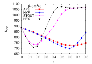
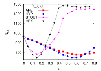
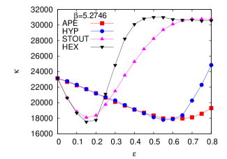
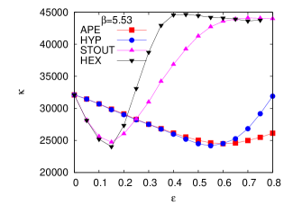
Interestingly, conjugate gradient inversion is also optimized at similar values of condit . In Figure 2 we show the number of conjugate gradient iterations required to invert a smeared staggered Dirac operator, , in a representative configuration drawn from thermalized ensembles. These results were obtained with a CG stopping criterion that the norm of the residual is less than . Note that the performance of the APE and HYP smeared operators are very similar to each other, just as before. The behaviour of the Stout and HEX smearing are also similar, but quite different from the previous pair. Again, the lattice spacing and pion mass seems to make little difference to the optimization.
Using the smeared staggered Dirac operator, , we found the minimum and maximum eigenvalues of : and . We defined the condition number . One expects that the number of CG iterations is closely related to , as indeed it is seen to be (see Figure 2). We found that is independent of to better than 1%, as expected, so is flat. The dependence of on is essentially due to the variation of .
We can use any of these criteria, namely, the minimization of , , or , to choose the best value of . The results are shown in Table 2 in different smearing schemes at different lattice spacings. There is a marginal decrease in the best smearing parameter in each scheme with decrease in lattice spacing. We see that there is reasonable agreement between the best values obtained through the three methods. Given this, we choose to work with the values for APE and HYP, and with for HEX and for Stout.
III.2 Smeared quarks and chirally symmetric correlators
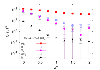
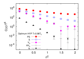
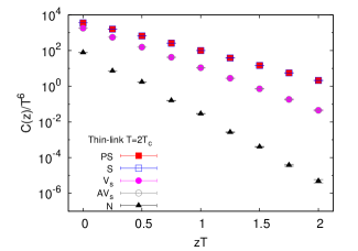
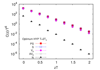
Chiral symmetry restoration in the high temperature phase of QCD is easily seen in hadronic correlation functions. Below the local meson correlators: S, PS, V, and AV are quite distinct, but above they collapse into one (see Figure 3). A pairwise degeneracy of the S/PS and V/AV shows chiral symmetry restoration, and has been demonstrated earlier as well with thin-link staggered valence quarks. However, the near-degeneracy of the two pairs at high temperature, visible only after smearing, is a new observation. This occurs in all the data sets: N, O, and P.
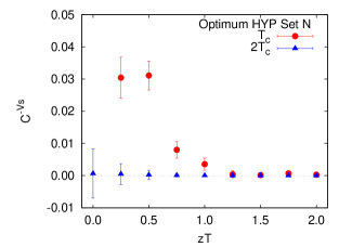
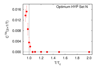
Pairwise degeneracy arising from chiral symmetry restoration is most easily seen in the vanishing of , and at high temperature quasi . On examining these combinations, it turns out that the degeneracy for becomes clearer with smearing. For example, is at with thin-link valence quarks, but becomes when optimal HYP smeared valence quarks are used. The improvement is most remarkable in the S/PS sector, where we found at using thin-link valence, but using optimal HYP smeared valence. At larger all the negative chiral projections vanished. It was seen earlier quasi that for vanished when , but remained non-zero at short distances. In Figure 4 we show this effect at and also, that it vanishes at . A more detailed view of the temperature dependence is exhibited by showing how changes with . Below the correlator does not vanish, but the spatial structure seems to have entirely disappeared for . This gives one definition of the width of the chiral crossover; it is larger than the one implied by (see Appendix A).
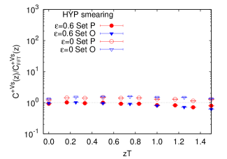
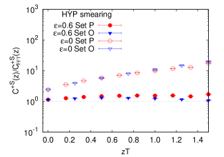
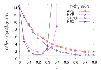
is close to the FFT prediction with either thin-link or smeared valence quarks. With thin-link staggered valence quarks, we see that is different from FFT, as previously observed. However, on smearing, they become compatible with FFT (see Figure 5). This is a more detailed understanding of why the meson screening correlators are nearly degenerate in Figure 3.
In Figure 6 we show that the correlator approaches FFT as the parameter is tuned to the optimum in each of the smearing schemes, approaching closest to FFT at the optimum. We used the distance in this demonstration because it is neither in the far IR nor in the UV. The optimum HYP and HEX schemes bring the correlator closer to FFT than the APE and Stout smearing schemes, although the latter also come very close to FFT. Next we explore this difference between schemes.
III.3 Smearing, taste symmetry and screening masses
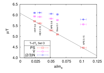
On examining screening masses, we found that they depend on the smearing parameter essentially only through the taste symmetry breaking measure
| (6) |
where the subscripts on the right denote the pion taste structure. The taste is the Goldstone pion. We chose the partner with taste structure as an indicator of taste splitting since it turned out to be relatively easily measured. Figure 7 shows the nearly linear dependence of on . The figure shows the clear superiority of the HEX scheme over Stout. Using the scaling shown in Figure 7, one could extrapolate screening masses to the limit . However, this is premature, since it involves an extrapolation to suboptimal values of . The S/PS screening masses obtained using local operators with dynamical p4 quarks at a comparable temperature turns out to be around edwin .
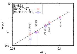
More information can be extracted from the taste-splitting of the screening masses at finite ,
| (7) |
The only previous study of this kind was reported in edwin . In Figure 7 we show as a function of . In making this comparison we held the lattice spacing fixed, with one set of measurements at , one at in set O and a third at in set P. We find over the range of values we obtained. This removes the ambiguity remarked upon in edwin .
One can argue for this on general grounds. A hadron mass, , can be written as , where we treat as a generic label for all the parameters which control smearing. A screening mass, , can be written as , since , or as . For data taken at fixed cutoff, , we need not show this parameter explicitly. Although we work at fixed , it is profitable to consider the dependence on this variable. A series expansion in near the chiral limit would yield different dependence for the Goldstone pion mass
| (8) |
where is any other mass scale, and the coefficients depend on . As a result, and . If taste symmetry were recovered in the chiral limit by tuning , then one might argue that and hence . This would also mean that all pion tastes are forced to be Goldstones, with an expansion starting at order . Chiral logarithms, which we have neglected here, could become important at smaller masses and spoil this scaling.
Even if smearing achieves a more limited goal of significantly decreasing at finite without actually recovering taste symmetry completely, one might still recover quadratic scaling. All that is needed is that and become much smaller than the actual taste splitting in the problem. In general one would have
| (9) |
The data in Figure 7 shows that and , are small compared to . This quantifies how well smearing works. The fact that it seems to work better at finite temperature than at with fixed values of and possibly indicates that the Dirac eigenvalue spectrum is simpler. We shall return to this point later.
The main conclusion from these studies of smearing is the following. Optimising the suppression of UV modes automatically improves taste symmetry in the hadron spectrum at . This leads to superlinear improvement in taste symmetry in the hot phase of QCD. In order to gain most from such an improvement, one should then choose the best possible smearing scheme. With partial quenching, as here, this would mean working with the optimized HYP scheme; with dynamical smeared quarks it would mean working with the optimized HEX scheme.
IV Results
IV.1 Hot QCD: weak coupling and the Dirac spectrum
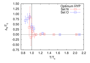
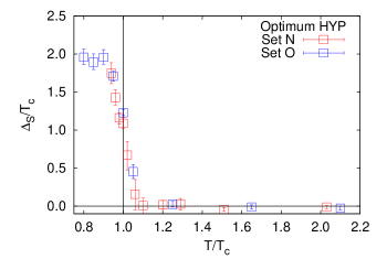
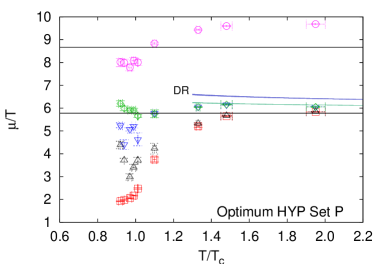
We found that the mass-splitting between chiral partners changes rapidly in the low-temperature phase and vanishes fairly close to in the hot phase. In Figure 8 we show that and both vanish at . Also, a comparison of sets N and O show very little quark mass dependence at about the same lattice spacing. These results are in contrast to the observations in quasi ; cheng that remains significantly non-zero up to a temperature significantly higher than . The change from the old results quasi using the same data set P, confirms that the improvement is due to smearing.
The rapid approach to behaviour similar to weak-coupling theory has implications for the spectrum of the staggered Dirac operator. The vanishing of the pion mass in the chiral limit at is related to a finite density of the Dirac eigenvalues near zero. It was shown earlier in a study of set O with thin-link quarks that a gap developed in the massless staggered eigenvalue spectrum a little above , and that the hot phase contained localized Dirac eigenvectors lacaze .
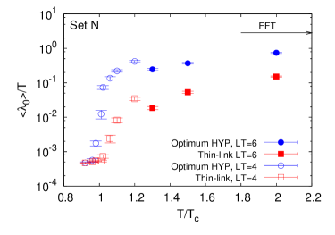
Here we studied the gap by measuring the smallest eigenvalue of the massless staggered Dirac operator, . The ensemble average, , at a given temperature was generally seen to be within a factor of four of the minimum over the ensemble. In view of this, we report . As can be seen in Figure 9, it climbs by two orders of magnitude between and for the smeared Dirac operator. For the thin-link operator, rises at significantly higher temperature.
One sees some volume dependence in the result. This was studied extensively in lacaze , where it was found that the volume dependence becomes negligible when the spatial size, , is of the order of . For , this would be at , which seems to happen at . In future it would be interesting to study this volume dependence further.
It is also of interest to note that becomes comparable to at with optimum HYP smearing. Since this happens for all the data sets, it accounts for the lack of quark mass dependence seen in and . With thin-link quarks this crossing is delayed to , thus affecting all screening phenomena.
In set N at we spotted one configuration out of the 50 for which was two orders of magnitude below . This implies the existence of a small fraction of atypical configurations in the thermal ensemble. These would be interesting in a study of axial U(1) symmetry at finite temperature, where such atypical configurations have been linked to topological configurations by observations with overlap oldlacaze or HISQ quarks in ohno . However, that would require a much larger statistical sample, and is therefore best left to the future.
IV.2 Comparison with weak-coupling theory
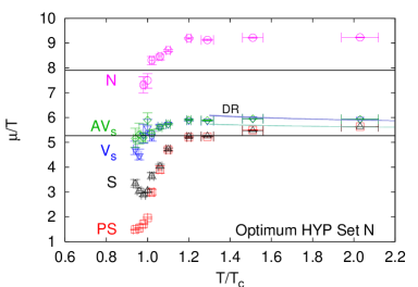
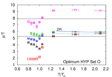
Finally, the results for the screening masses as functions of are shown in Figure 10 for all three data sets with optimal HYP smearing. Also shown are the values expected in FFT on lattices with the same size. The analysis of correlation functions obtained with these smeared valence quarks shows that the screening masses in all channels approach FFT at high . The most striking new feature of this data is that this approach is from above, in conformity with the predictions of dr . Similar results are obtained with optimal HEX smeared quarks. We have shown earlier in Figure 7 that there is a remaining uncertainty of around 15% in the determination of the the S/PS screening mass. This comes from the residual taste symmetry breaking at the best optimization of the screening parameters possible at this lattice spacing. Reduction of this uncertainty requires going to finer lattices.
The weak coupling prediction for the meson-like screening masses is
| (10) |
Here is the 2-loop QCD coupling evaluated in the scheme at the scale . for two flavours of quarks in a dimensional reduction (DR) scheme dr . A hard thermal loop (HTL) resummation which neglects soft gluon contributions to the vertex yields htl . These weak-coupling predictions are also shown in Figure 10, with determined using tscale . As one can see, both the weak-coupling predictions are close to the observed screening masses.
V Conclusions
Several properties of quarks at experimentally accessible temperatures above seem to be explained in weak coupling QCD. However, one which showed puzzling departures from weak-coupling predictions was screening masses from hadronic excitations. In quenched computations it was seen that the results depended strongly on the kind of valence quark used scrnp . With this clue in hand we performed computations with dynamical staggered sea quarks and improved valence quarks in three sets of computations, one new (set N, see Table 1) and two older, (sets O nt4 and P nt6 ). Studies with staggered valence quarks were reported earlier with set P quasi .
A preliminary part of this work was the optimization of the valence quarks. We used four popular versions of fat-link staggered quarks. We optimized the smearing parameter, , in each case by observing changes to the power spectrum of the plaquette (see Figure 1) and the largest and smallest eigenvalues of the Dirac operator (see Figure 2). The optimum was chosen so that the UV was suppressed as much as possible without changing the IR behaviour in both cases. This also improved the performance of the conjugate gradient algorithm used for the inversion of the Dirac operator (see Table 2). Such a tuning was done at . We found mild changes in the tuning parameters as the lattice spacing was changed by a factor of 2.
Although the smearing parameter is optimized by requiring that the IR components of fields do not change appreciably, it does affect the long-distance properties of the theory, such as masses. We compared different schemes through a measure of the recovery of staggered quark taste symmetry in the spectrum of pions (see Figure 7). The optimized HYP smearing works best, although optimized HEX smearing comes a close second. This is pleasant, since dynamical simulations with HEX smearing are easier than with HYP.
Smearing causes systematic changes in finite temperature properties of interest. We found that the screening mass in the hot phase increases systematically as taste symmetry breaking is reduced at (see Figure 7). Also, taste symmetry breaking in the hot phase improves super-linearly with improvement at (see Figure 7). Since recovery of taste symmetry has been used as the main indicator of the reduction of UV effects, it is natural in this study to use optimized HYP smearing in order to best reduce lattice artifacts.
On doing this we find that the screening correlator recovers the degeneracies that a theory of weakly coupled fermions would predict (see Figure 3). This happens very close to, and above, (see Figure 4). The correlators themselves are also close to the predictions of a free fermion field theory (see Figure 5). Consistent with this, the screening masses at high temperature are found to be close to weak-coupling theory (see Figure 10). A computation in dimensional reduction dr gives results which are slightly different from a HTL computation neglecting soft-gluon effects on the vertex htl . The lattice computation is unable to distinguish these as yet, but we may expect this to improve in the near future.
We also see that the smallest eigenvalue of the optimally HYP smeared massless staggered Dirac operator shows a rapid jump from extremely small values in the mean below to fairly large values above (see Figure 9). The behaviour of the thin-link staggered operator is qualitatively similar, although quantitatively slower to change. Since the smallest eigenvalue of the massless smeared operator is comparable to the bare mass already at , the limit of physical renormalized mass becomes easy to take in the high temperature phase. There is evidence for a very small fraction of completely atypical configurations in the hot phase. A study of the topology of these gauge configurations lies outside the scope of this paper.
The lattice computations described here were performed on the Cray X1 of the ILGTI in TIFR. We thank Ajay Salve and Kapil Ghadiali for technical assistance. We also thank Debasish Banerjee, Saumen Datta, Mikko Laine, Nilmani Mathur, Subroto Pal and Christian Schmidt for their comments. Some of the configurations used in this study were generated earlier for other studies by the ILGTI.
Appendix A Determination of
| 5.2747(6) | 0.009(2) | |
| 5.2743(5) | 0.006(1) | |
| 5.2741(5) | 0.006(1) | |
| 5.2743(6) | 0.007(1) |
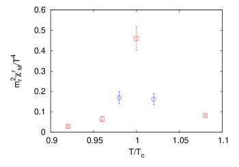
The cross over is determined at for a bare quark mass , where is the lattice spacing at . We determined by positions of the peaks of different susceptibilities. was defined to be the full width at half maximum (FWHM) of the same susceptibilities.
We measured the Wilson line susceptibility, nt6 , the bare chiral susceptibility, laermanntherm , the corresponding renormalized quantity fodor1 , and the fourth order QNS, and nt4 , at various values of in the crossover region. For the measurement of , we determined the chiral condensate at zero temperature on lattice at the same values of as the finite temperature ones.
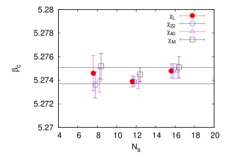
Prior to the runs listed in Table 1, we performed a series of runs at fixed bare quark mass, , with and 12. We used these runs to make first estimates of , and followed up with the runs along lines of constant listed in Table 1. The compatibility of these runs is shown in Figure 11, where is given as a function of . The figure also shows that with this cutoff, the deconfining and chiral cross overs in QCD coincide; peaks between 0.98 and .
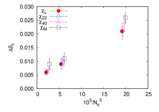
To determine accurately, we interpolated data for susceptibilities using multihistogram reweighting swnsn in the cross over region. From bootstrap resampling of the histograms, we determined the means and errors in the position of the peak of each susceptibility and its FWHM, so obtaining and largeNc . We found and for each of the susceptibilities on the three different lattice volumes. The results of which are shown in Figure 12. Since we found very little volume dependence in , we made a fit to a constant, independent of volume. The values of so determined are displayed in Table 3. In Figure 12 we also show the volume dependence of . This decreases with the volume, and gives some indication of saturating, within errors, close to our largest lattice. So we take obtained on , as our best estimate. These estimates are also listed in Table 3. We find that the variation in with different susceptibilities occur well within the width of the cross over measured from each indicator separately. In fact, the four estimates of are consistent with each other within 68% confidence limits. Combining all four measurements, we quote and .
References
-
(1)
J. P. Blaizot et al., Phys. Lett. B 523, 143 (2001);
A. Vuorinen, Phys. Rev. D67, 074032 (2003);
Y. Schroder and M. Laine, hep-lat/0509104. - (2) C. E. Detar and J. B. Kogut, Phys. Rev. Lett. 59, 399 (1987).
- (3) K. D. Born et al., Phys. Rev. Lett. 67, 302 (1991).
- (4) D. Banerjee et al., Phys. Rev. D83, 074510 (2011).
- (5) M. Cheng et al., Eur. Phys. J. C 71, 1564 (2011).
- (6) E. Laermann and F. Pucci, Eur. Phys. J. C 72, 2200 (2012).
- (7) B. B. Brandt et al., arxiv:1210.6972.
- (8) M. Laine and M. Vepsäläinen, J. H. E. P. 0402, 004 (2004).
- (9) W. M. Alberico et al., Nucl. Phys. A 792, 152 (2007).
- (10) S. Datta et al., arxiv:1212.2927.
- (11) M. Albanese et al., Phys. Lett. B 192, 163 (1987).
- (12) A. Hasenfratz and F. Knechtli, Phys. Rev. D64, 034504 (2001).
- (13) C. Morningstar and M. J. Peardon, Phys. Rev. D69, 054501 (2004).
- (14) S. Capitani, S. Dürr, C. Hoelbling, J. H. E. P. 0611, 028 (2006).
-
(15)
K. Orginos, D. Toussaint and R. L. Sugar, Phys. Rev. D60, 054503 (1999);
E. Follana et al., eprint hep-lat/0406021;
T. Bae et al., Phys. Rev. D77, 094508 (2008). - (16) R. V. Gavai and S. Gupta, Phys. Rev. D71, 114014 (2005).
- (17) R. V. Gavai and S. Gupta, Phys. Rev. D78, 114503 (2008).
- (18) G. H. Golub and C. F. van Loan, Matrix Computations, Johns Hopkins University Press (1996).
- (19) M. F. L. Golterman, Nucl. Phys. B 273, 663 (1986).
- (20) T. Kurth et al., arxiv:1011.1780.
- (21) R. V. Gavai, S. Gupta and R. Lacaze, Phys. Rev. D77, 114506 (2008).
- (22) R. V. Gavai, S. Gupta and R. Lacaze, Phys. Rev. D65, 094504 (2002).
- (23) H. Ohno et al., arxiv:1211.2591.
- (24) S. Gupta, Phys. Rev. D64, 034507 (2001).
- (25) E. Laermann, Nucl. Phys. Proc. Suppl. 63, 114 (1998).
- (26) Y. Aoki et al., Phys. Lett. B 643, 46 (2006).
- (27) A. M. Ferrenberg and R. H. Swendsen, Phys. Rev. Lett. 63, 1195 (1989).
- (28) S. Datta and S. Gupta, Phys. Rev. D80, 114504 (2009).