Bloch-wave homogenization on large time scales and dispersive effective wave equations

Abstract

We investigate second order linear wave equations in periodic media, aiming at the derivation of effective equations in $\mathbb{R}^{n}$, $n\in\{1,2,3\}$. Standard homogenization theory provides, for the limit of a small periodicity length $\varepsilon>0$, an effective second order wave equation that describes solutions on time intervals $[0,T]$. In order to approximate solutions on large time intervals $[0,T\varepsilon^{-2}]$, one has to use a dispersive, higher order wave equation. In this work, we provide a well-posed, weakly dispersive effective equation, and an estimate for errors between the solution of the original heterogeneous problem and the solution of the dispersive wave equation. We use Bloch-wave analysis to identify a family of relevant limit models and introduce an approach to select a well-posed effective model under symmetry assumptions on the periodic structure. The analytical results are confirmed and illustrated by numerical tests.

Keywords: homogenization, wave equation, weakly dispersive model, Bloch-wave expansion

MSC: 35B27, 35L05

1 Introduction

The wave equation describes wave propagation in very different applications, ranging from elastic waves to electro-magnetic waves. In some applications, it is of interest to describe waves in periodic media, where the period $\varepsilon>0$ is much smaller than the wave-length. The most fundamental questions regard the effective wave speed and the dispersive behavior due to the heterogeneities.

We concentrate on the simplest model, the second order wave equation in divergence form. For notational convenience, we restrict ourselves to a unit density coefficient and study, for $x\in\mathbb{R}^{n}$, the wave equation

$$\partial_{t}^{2}u^{\varepsilon}(x,t)=\nabla\cdot(a^{\varepsilon}(x)\nabla u^{\varepsilon}(x,t))\,.$$ (1.1)

The medium is characterized by a positive coefficient matrix $a^{\varepsilon}:\mathbb{R}^{n}\to\mathbb{R}^{n\times n}$. We are interested in periodic media with a small periodicity length-scale $\varepsilon>0$, and assume that $a^{\varepsilon}(x)=a_{Y}(x/\varepsilon)$, where $a_{Y}:\mathbb{R}^{n}\to\mathbb{R}^{n\times n}$ is periodic. The wave equation is complemented with the initial condition

$$u^{\varepsilon}(x,0)=f(x),\quad\partial_{t}u^{\varepsilon}(x,0)=0\,.$$ (1.2)

Assumption 1.1.

On the initial data we assume that $f\in L^{2}(\mathbb{R}^{n})\cap L^{1}(\mathbb{R}^{n})$ has the Fourier representation

$$f(x)=\frac{1}{(2\pi)^{n/2}}\int_{\mathbb{R}^{n}}F_{0}(k)\,e^{+{\rm i}k\cdot x}\,dk\,,$$ (1.3)

where the function $F_{0}:\mathbb{R}^{n}\to\mathbb{C}$ is supported on the compact set $K\subset\subset\mathbb{R}^{n}$.

On the coefficient $a_{Y}:\mathbb{R}^{n}\to\mathbb{R}^{n\times n}$ we assume $Y$-periodicity for the cube $Y:=(-\pi,\pi)^{n}\subset\mathbb{R}^{n}$ and the regularity $a_{Y}\in C^{1}(\mathbb{R}^{n},\mathbb{R}^{n\times n})$. Moreover, we assume that $a_{Y}(y)$ is a symmetric and positive definite matrix field: for some $\gamma>0$ there holds $(a_{Y}(y))_{ij}=(a_{Y}(y))_{ji}$ for all $i,j\in\{1,...,n\}$ and $\sum_{i,j=1}^{n}(a_{Y}(y))_{ij}\xi_{i}\xi_{j}\geq\gamma|\xi|^{2}$ for every $y\in\mathbb{R}^{n}$ and all $\xi\in\mathbb{R}^{n}$.

The set $Y\subset\mathbb{R}^{n}$, the reciprocal cell $Z:=(-1/2,1/2)^{n}\subset\mathbb{R}^{n}$, and the support $K\subset\mathbb{R}^{n}$ are fixed data of the problem.

The Fourier transform is always understood in the sense of $L^{2}(\mathbb{R}^{n})$. We note that $F_{0}$ is bounded because of $f\in L^{1}(\mathbb{R}^{n})$. Since $F_{0}$ has compact support, every derivative of $f$ is of class $L^{2}(\mathbb{R}^{n})$, hence $f\in C^{\infty}(\mathbb{R}^{n})$. We will later restrict ourselves to dimensions $n\leq 3$, an assumption that is used in Sobolev-embeddings. General dimensions can be treated under stronger regularity assumptions on $a_{Y}$.

The fundamental question of homogenization theory is the following: For small $\varepsilon>0$, can the solution $u^{\varepsilon}$ be approximated by a solution of an equation with constant coefficients? The answer is affirmative: There exists an effective coefficient matrix $A\in\mathbb{R}^{n\times n}$, computable from $a_{Y}$, such that the following holds: on an arbitrary time interval $[0,T]$, if $w:\mathbb{R}^{n}\times[0,T]\to\mathbb{R}$ is the solution of

$$\partial_{t}^{2}w(x,t)=\nabla\cdot(A\nabla w(x,t))\,,\quad w(x,0)=f(x),\quad\partial_{t}w(x,0)=0\,,$$ (1.4)

there holds $u^{\varepsilon}\to w$ as $\varepsilon\to 0$. For the result and function spaces see e.g. [6].

We are interested in a refinement of this result. Our aim is to investigate the behavior of solutions $u^{\varepsilon}$ of (1.1) for large times, namely for all $t\in[0,T_{0}\varepsilon^{-2}]$ with $T_{0}>0$. It is well-known that the homogenized equation (1.4) cannot provide an approximation of $u^{\varepsilon}$ on the interval $[0,T_{0}\varepsilon^{-2}]$. Instead, we need a dispersive equation to approximate $u^{\varepsilon}$.

Main result.

In addition to the coefficient matrix $A\in\mathbb{R}^{n\times n}$, we will define $E\in\mathbb{R}^{n\times n}$ and $F\in\mathbb{R}^{n\times n\times n\times n}$, computable from the coefficient $a_{Y}(.)$ with the Bloch eigenvalue problem on the periodicity cell $Y$. The constant coefficient matrices define linear spatial differential operators: the two second order operators $AD^{2}=\sum_{i,j}A_{ij}\partial_{i}\partial_{j}$ and $ED^{2}=\sum_{i,j}E_{ij}\partial_{i}\partial_{j}$, and the fourth order operator $FD^{4}=\sum_{i,j,m,l}F_{ijml}\partial_{i}\partial_{j}\partial_{m}\partial_{l}$. The weakly dispersive effective equation reads

$$\partial_{t}^{2}w^{\varepsilon}=AD^{2}w^{\varepsilon}+\varepsilon^{2}ED^{2}\partial_{t}^{2}w^{\varepsilon}-\varepsilon^{2}FD^{4}w^{\varepsilon}\,.$$ (1.5)

As initial conditions we use once more $w^{\varepsilon}(x,0)=f(x)$ and $\partial_{t}w^{\varepsilon}(x,0)=0$. Equation (1.5) is of fourth order in the spatial variables, and it contains a term that uses second spatial and second time derivatives. The operator contains the small parameter $\varepsilon>0$ explicitly. It can nevertheless be regarded as an effective equation in the sense of homogenization theory, since the coefficients are $x$-independent. Numerically, (1.5) is much easier to solve than (1.1), since the fine scale need not be resolved. The contributions of higher order (operators with factor $\varepsilon^{2}$) describe the (weak) dispersive effects due to the heterogeneity of the medium. Formally, for $\varepsilon=0$, we recover the homogenized equation (1.4).

Our main result shows that the weakly dispersive equation (1.5) provides, for large times, an approximation of the original equation (1.1). To our knowledge, both aspects of our theorem are new in dimension $n>1$: (i) the specification of a well-posed weakly dispersive effective wave equation and (ii) the rigorous proof of the homogenization error estimate on large time scales.

Theorem 1.2.

Let $\varepsilon=\varepsilon_{l}\to 0$ be a sequence of positive numbers and $n\in\{1,2,3\}$ be the dimension. Let the medium $a_{Y}:\mathbb{R}^{n}\to\mathbb{R}^{n\times n}$ and the initial data $f:\mathbb{R}^{n}\to\mathbb{R}$ satisfy Assumption 1.1. We assume that $y\mapsto a_{Y}(y)$ is symmetric under reflections $y_{j}\longleftrightarrow-y_{j}$, and symmetric under coordinate exchanges $y_{j}\longleftrightarrow y_{k}$, see (2.27).

We use the coefficient matrices $A$ and $C$ defined in (2.22), $E$ and $F$ as defined in Lemma 3.1. Then the following holds:

1. Well-posedness Equation (1.5) with initial condition (1.2) has a unique solution $w^{\varepsilon}$ for all positive times (see Theorem 3.3 for function spaces).

2. Error estimate Let $w^{\varepsilon}$ be the solution of (1.5), and let $u^{\varepsilon}$ be the solution of (1.1) for the same initial condition (1.2). Then, with a constant $C_{0}=C_{0}(a_{Y},T_{0},f)$, there holds the error estimate

   $$\sup_{t\in[0,T_{0}\varepsilon^{-2}]}\|u^{\varepsilon}(.,t)-w^{\varepsilon}(.,t)\|_{L^{2}(\mathbb{R}^{n})+L^{\infty}(\mathbb{R}^{n})}\leq C_{0}\varepsilon\,.$$ (1.6)

The definition of the norm in (1.6) is recalled at the end of Section 2.2. The $L^{2}(\mathbb{R}^{n})$-norm is a result of the Bloch-wave expansion (it appears e.g. in Theorem 2.2), while the $L^{\infty}(\mathbb{R}^{n})$-norm appears in the control of error terms after Theorem 2.4, but also in energy estimates, see Lemma 3.4.

Comparison with the literature

The derivation of effective equations in periodic homogenization problems is an old subject [25], two-scale convergence [2] is today the most relevant analytical tool. The use of Bloch-wave expansions [29] was explored only more recently, see e.g. [9, 10, 11].

Compared to elliptic and parabolic equations, some distinctive features are relevant in the analysis of the wave equation. One observation of [6] was that convergence of energies can only be expected for initial data that are adapted to the periodic medium, see also [18]. Diffraction and dispersion effects are analyzed in the spirit of homogenization theory in [3, 5]. While the underlying questions are similar, these contributions study a different scaling behavior in $\varepsilon$. Other homogenization results for the wave equation are contained in [7, 19, 22, 23, 27, 28].

The study of dispersive effects and the derivation of a dispersive effective wave equation are central aims in the works of Chen, Fish, and Nagai, e.g. [14, 15, 16, 17]. The authors expand several ideas to treat the problem, among others they propose to introduce a slow and a fast time scale to capture the long-time behavior of waves. The authors concentrate on numerical studies and do not provide a derivation of an effective model.

Derivation of dispersive models.

To our knowledge, the first rigorous result that establishes a dispersive model for the wave equation in the scaling of (1.1) appeared in [20]. In that contribution, the one-dimensional case $n=1$ was analyzed, the one-dimensional version of (1.5) was formulated (in this case, $A$, $E$, and $F$ are scalar coefficients and the differential operator is $D=\partial_{x}$), and a result similar to our Theorem 1.2 was shown: the well-posedness of the dispersive equation and an error bound on large time intervals.

Beyond the one dimensional case, we are not aware of any rigorous results. The most relevant contribution with the perspective taken here is [26]. In that paper, Bloch-wave expansions are used to analyze the problem, mathematical insight is gained, and the dispersive wave equation (3.1) is formulated (not in one of the theorems, but as a formal consequence on page 992). We use many of the ideas of that contribution.

Equation (3.1) appears also as equation (42) in [17], the authors call it the “bad” Boussinesq equation. The problem about this equation is its ill-posedness: Loosely speaking, the equation is of the form $\partial_{t}^{2}u+Lu=0$, with $L=-\Delta-\varepsilon^{2}\Delta^{2}$. The lowest order part (in $\varepsilon$) of $L$ is $-\Delta$, hence a positive operator, but for every $\varepsilon>0$, the operator is negative, since $\Delta^{2}$ is positive and contains the highest order of differentiation. One can speculate that this was the reason why no effective dispersive models were rigorously formulated in the above mentioned works.

It was already observed in [17], that a “good” Boussinesq equation can be obtained with a simple trick: Going back to the prototype problem $\partial_{t}^{2}u=-Lu=\Delta u+\varepsilon^{2}\Delta^{2}u$, we replace $\Delta u$ to lowest order (in $\varepsilon$) by $\partial_{t}^{2}u$ and write the equation as $\partial_{t}^{2}u=\Delta u+\varepsilon^{2}\Delta\partial_{t}^{2}u$. In this form, the equation is well-posed. This observation was also exploited in [20], where it was shown rigorously that the “good” Boussinesq equation is the effective model for large times in the one-dimensional case.

In this contribution we treat the higher dimensional case, using methods that are completely different from those of [20]. Our new results rely on a Bloch-wave expansion of the solution $u^{\varepsilon}$, which we analyze in Sections 2.1–2.3; in this part we follow closely the ideas of [26]. To clearify the connection to this well-known article, we repeat that no convergence result appears in [26], function spaces and assumptions are not always clearly specified in [26], and only the “bad” Boussinesq equation appears (with a wrong sign and without further discussion) in [26].

We have to introduce two assumptions: (i) inital data are compactly supported in Fourier space and (ii) the heterogeneous medium has certain symmetries in the cell $Y$. Both assumptions can possibly be relaxed with some additional effort and new decomposition techniques; our aim here is to present the long-time homogenization result in the simplest relevant case. Due to the multi-dimensional setting, we have anyway to work with tensors of coefficients to transform the “bad” effective equation into the “good” one. We show with mathematical rigor that the weakly dispersive effective equation has the approximation property for large times.

In Section 2 we expand the solution $u^{\varepsilon}$ in Bloch waves, in Section 3 we analyze the weakly dispersive equation (1.5). The proof of Theorem 1.2 is concluded at the end of Section 3. Section 4 contains numerical results.

2 Approximation with a Bloch wave expansion

In this section we present, in slightly changed notation and with mathematical rigor regarding assumptions and norms, the approximation results of [26]. To simplify some of the notation of [26], we consider here only the mass-density $\bar{\rho}\equiv 1$ and the scaling factor $\lambda=1$.

2.1 Bloch wave expansion

We are given a periodic medium by the coefficient matrix $a_{Y}(y)$ on the cube $Y$. The Bloch wave expansion uses functions $\psi_{m}$, which are solutions of a periodic eigenvalue problem on $Y$. The wave parameter $k$ is a vector in the reciprocal periodicity cell $Z=(-1/2,1/2)^{n}$. At this point, we regard $k\in Z$ as a given parameter and consider

$$-(\nabla_{y}+{\rm i}k)\cdot(a_{Y}(y)(\nabla_{y}+{\rm i}k)\psi_{m}(y,k))=\mu_{m}(k)\psi_{m}(y,k)\,.$$ (2.1)

We search for $\psi_{m}(.,k):Y\to\mathbb{C}$ in the space $H^{1}_{\mathrm{per}}(Y)$, defined as the space of periodic functions on $Y$ of class $H^{1}$. We find a family (indexed by $m\in\mathbb{N}=\{0,1,2,\dots\}$) of periodic solutions $\psi_{m}(.,k):Y\to\mathbb{C}$ with non-negative real eigenvalues $\mu_{m}(k)$, $\mu_{m+1}(k)\geq\mu_{m}(k)$, both the solution and the eigenvalue depend on $k$. We assume that the functions are normalized in $L^{2}(Y)$, $\|\psi_{m}\|_{L^{2}(Y)}=1$. Regarding the regularity of $\psi_{m}$ we note that, for $a_{Y}$ of class $C^{1}$, standard elliptic regularity theory implies $\psi_{m}\in H^{2}(Y)$.

Based on the eigenfunction $\psi_{m}$, we can construct the quasi-periodic Bloch-waves $w_{m}(y,k):=\psi_{m}(y,k)e^{{\rm i}k\cdot y}$, which satisfy

$$-\nabla_{y}\cdot(a_{Y}(y)\nabla_{y}w_{m}(y,k))=\mu_{m}(k)w_{m}(y,k).$$ (2.2)

We recall an essential fact regarding the completeness of these eigenfunctions (see e.g. [11] for this well-known result). The Bloch waves form a basis of $L^{2}(\mathbb{R}^{n})$ in the sense that every function $g\in L^{2}(\mathbb{R}^{n})$ can be expanded as

$$g(y)=\sum_{m=0}^{\infty}\int_{Z}\hat{g}_{m}(k)w_{m}(y,k)\,dk\,,\qquad\hat{g}_{m}(k)=\int_{\mathbb{R}^{n}}g(y)w_{m}(y,k)^{*}\,dy\,,$$ (2.3)

where we use the star ^∗ to denote complex conjugation and the first equality is understood in the sense of $L^{2}(\mathbb{R}^{n})$-convergence of partial sums. There holds the Parseval identity

$$\|g\|_{L^{2}(\mathbb{R}^{n})}^{2}=\int_{\mathbb{R}^{n}}|g(x)|^{2}\,dx=\sum_{m=0}^{\infty}\int_{Z}|\hat{g}_{m}(k)|^{2}\,dk=\|\hat{g}\|_{l^{2}(\mathbb{N},L^{2}(Z))}^{2}\,.$$ (2.4)

Rescaled Bloch wave expansion

We investigate a strongly heterogeneous medium $a^{\varepsilon}(x)=a_{Y}(x/\varepsilon)$. Starting from the Bloch waves on the cube $Y$, we define rescaled quantities as

$$\psi_{m}^{\varepsilon}(x,k):=\psi_{m}\left(\frac{x}{\varepsilon},\varepsilon k\right)\,,\quad\mu_{m}^{\varepsilon}(k):=\frac{1}{\varepsilon^{2}}\mu_{m}(\varepsilon k)\,,$$ (2.5)

$$w_{m}^{\varepsilon}(x,k):=w_{m}\left(\frac{x}{\varepsilon},\varepsilon k\right)=\psi_{m}^{\varepsilon}(x,k)e^{{\rm i}k\cdot x}=\psi_{m}\left(\frac{x}{\varepsilon},\varepsilon k\right)e^{{\rm i}k\cdot x}\,.$$ (2.6)

This choice guarantees, in particular,

$$-\nabla\cdot(a^{\varepsilon}(x)\nabla w_{m}^{\varepsilon}(x,k))=\mu_{m}^{\varepsilon}(k)w_{m}^{\varepsilon}(x,k).$$ (2.7)

The expansion formula (2.3) in Bloch eigenfunctions can be expressed in the new variables. Every function $f\in L^{2}(\mathbb{R}^{n})$ can be written as

$$f(x)=\sum_{m=0}^{\infty}\int_{Z/\varepsilon}\hat{f}_{m}^{\varepsilon}(k)w_{m}^{\varepsilon}(x,k)\,dk\,,\qquad\hat{f}_{m}^{\varepsilon}(k)=\int_{\mathbb{R}^{n}}f(x)w_{m}^{\varepsilon}(x,k)^{*}\,dx\,.$$ (2.8)

To verify this formula, it suffices to set $f(x)=g(x/\varepsilon)$ and $\hat{f}_{m}^{\varepsilon}(k)=\varepsilon^{n}\hat{g}_{m}(\varepsilon k)$ and to use (2.3). This shows additionally the Parseval identity in transformed variables,

$$\|f\|_{L^{2}(\mathbb{R}^{n})}^{2}=\int_{\mathbb{R}^{n}}|f(x)|^{2}\,dx=\sum_{m=0}^{\infty}\int_{Z/\varepsilon}|\hat{f}_{m}^{\varepsilon}(k)|^{2}\,dk=\|\hat{f}^{\varepsilon}\|_{l^{2}(\mathbb{N},L^{2}(Z/\varepsilon))}^{2}\,.$$ (2.9)

In our situation of $a_{Y}\in C^{1}(\mathbb{R}^{n},\mathbb{R}^{n\times n})$ and $f\in H^{2}(\mathbb{R}^{n})$, the series in (2.8) is also convergent in $H^{1}(\mathbb{R}^{n})$. We provide a proof in Appendix A.

Expansion of the solution

The Bloch-wave formalism can provide a formula for the solution of the original wave equation.

Lemma 2.1 (Expansion of the solution).

Let the medium $a_{Y}:\mathbb{R}^{n}\to\mathbb{R}^{n\times n}$ and the initial data $f:\mathbb{R}^{n}\to\mathbb{R}$ satisfy Assumption 1.1. Then, for every $\varepsilon>0$ and every $T_{\varepsilon}\in(0,\infty)$, the wave equation (1.1) has a unique weak solution $u^{\varepsilon}$ with the regularity $u^{\varepsilon}(x,t)\in L^{\infty}(0,T_{\varepsilon};H^{2}(\mathbb{R}^{n}))\cap W^{1,\infty}(0,T_{\varepsilon};H^{1}(\mathbb{R}^{n}))\cap W^{2,\infty}(0,T_{\varepsilon};L^{2}(\mathbb{R}^{n}))$.

The solution $u^{\varepsilon}$ of (1.1) can be represented as

$$u^{\varepsilon}(x,t)=\sum_{m=0}^{\infty}\int_{Z/\varepsilon}\hat{f}_{m}^{\varepsilon}(k)\,w_{m}^{\varepsilon}(x,k)\,\mathrm{Re}\left(e^{{\rm i}t\sqrt{\mu_{m}^{\varepsilon}(k)}}\right)\,dk\,.$$ (2.10)

Here, the right hand side is understood as the strong $L^{2}(\mathbb{R}^{n})$-limit of partial sums, for every fixed $t\geq 0$, and $\mathrm{Re}(.)$ denotes the real part.

Before we start the proof, we note that the expression in (2.10) formally defines a solution of (1.1)–(1.3). In fact, the second time derivative of the right hand side is given by the same formula, introducing only the additional factor $-\mu_{m}^{\varepsilon}(k)$ under the integral. On the other hand, the application of the operator $\nabla\cdot(a^{\varepsilon}(x)\nabla)$ to the integrand produces, by (2.7), the same result.

Proof.

Step 1. The weak solution. A weak solution $u^{\varepsilon}$ can be constructed, e.g., with a Galerkin scheme. One exploits the energy estimate which is obtained with a multiplication of equation (1.1) by the real function $\partial_{t}u^{\varepsilon}$,

$$0=\int_{\mathbb{R}^{n}}[\partial_{t}^{2}u^{\varepsilon}(.,t)-\nabla\cdot(a^{\varepsilon}(.)\nabla u^{\varepsilon}(.,t))]\partial_{t}u^{\varepsilon}=\frac{d}{dt}\frac{1}{2}\int_{\mathbb{R}^{n}}|\partial_{t}u^{\varepsilon}(t)|^{2}+|\nabla u^{\varepsilon}(t)|_{a^{\varepsilon}}^{2}\,,$$

where the last equality holds, since $a^{\varepsilon}(x)$ is a symmetric matrix for every $x\in\mathbb{R}^{n}$. Here and below we use the notation $|\xi|^{2}_{a}:=\xi^{*}\cdot(a\cdot\xi)$ for vectors $\xi\in\mathbb{C}^{n}$ and matrices $a\in\mathbb{R}^{n\times n}$. Also higher order estimates can be obtained. We use $L^{\varepsilon}:=\nabla\cdot(a^{\varepsilon}(x)\nabla)$ and multiply the equation $\partial_{t}^{2}u^{\varepsilon}=L^{\varepsilon}u^{\varepsilon}$ by $-\partial_{t}(L^{\varepsilon}u^{\varepsilon})$ to find

$$\frac{d}{dt}\frac{1}{2}\int|\partial_{t}\nabla u^{\varepsilon}|_{a^{\varepsilon}}^{2}+|L^{\varepsilon}u^{\varepsilon}|^{2}=0\,.$$ (2.11)

Since the initial data are $u|_{t=0}=f\in H^{2}(\mathbb{R}^{n})$ and $\partial_{t}u|_{t=0}=0$, we obtain estimates for $u^{\varepsilon}$ in the function spaces that are stated in the Theorem. The estimates for $L^{\varepsilon}u^{\varepsilon}(.,t)=\partial_{t}^{2}u^{\varepsilon}(.,t)\in L^{2}(\mathbb{R}^{n})$ imply the regularity $u^{\varepsilon}\in W^{2,\infty}(0,T_{\varepsilon};L^{2}(\mathbb{R}^{n}))$ and the estimates for $u^{\varepsilon}(.,t)\in H^{2}(\mathbb{R}^{n})$ due to $a_{Y}\in C^{1}(Y,\mathbb{R}^{n\times n})$ by standard elliptic regularity theory. Uniqueness within the given class follows from linearity, repeating the above calculations for differences of solutions.

Step 2. Convergence in (2.10). The Parseval identity (2.9) implies that the coefficient functions define an element $(\hat{f}^{\varepsilon}_{m}(k))_{m,k}$ of $l^{2}(\mathbb{N},L^{2}(Z/\varepsilon))$. As a consequence, also the modified coefficients $\left(\hat{f}^{\varepsilon}_{m}(k)\mathrm{Re}\left(e^{{\rm i}t\sqrt{\mu_{m}^{\varepsilon}(k)}}\right)\right)_{m,k}$ define an element in the same space, since all factors have absolute value bounded by $1$. Using again the Parseval identity (2.9), we conclude that the sum of (2.10) converges in $L^{2}(\mathbb{R}^{n})$, independently of $t\geq 0$.

Step 3. Identification of $u^{\varepsilon}$. We consider a partial sum $\sum_{m=1}^{M}$ in (2.10) to define a function $u^{\varepsilon}_{M}$ and observe that this provides a strong solution $u^{\varepsilon}_{M}$ of the wave equation to the initial values $f_{M}=\sum_{m=0}^{M}\int_{Z/\varepsilon}\hat{f}_{m}^{\varepsilon}(k)w_{m}^{\varepsilon}(x,k)\,dk$ and vanishing initial velocity. This fact can be checked with a direct calculation: the operator $\nabla\cdot(a^{\varepsilon}(x)\nabla)$ is understood in the weak form and can be applied to the $H^{1}(Y)$-functions $w_{m}^{\varepsilon}$. We claim that $u^{\varepsilon}_{M}$ forms a Cauchy sequence in the space $L^{\infty}([0,T_{\varepsilon}],H^{1}(\mathbb{R}^{n}))$. This follows with a testing argument, exploiting

$$\int_{\mathbb{R}^{n}}|\nabla u^{\varepsilon}_{M}(t)-\nabla u^{\varepsilon}_{N}(t)|_{a^{\varepsilon}}^{2}+|\partial_{t}u^{\varepsilon}_{M}(t)-\partial_{t}u^{\varepsilon}_{N}(t)|^{2}=\int_{\mathbb{R}^{n}}|\nabla f^{\varepsilon}_{M}-\nabla f^{\varepsilon}_{N}|_{a^{\varepsilon}}^{2}\to 0$$

for $M,N\to\infty$ due to the $H^{1}(\mathbb{R}^{n})$-convergence in (2.8). We conclude that $u^{\varepsilon}_{M}$ converges to a limit function. The limit function is again a weak solution of the wave equation, from the uniqueness of weak solutions we conclude $u^{\varepsilon}_{M}\to u^{\varepsilon}$ for $M\to\infty$.

On the other hand, as observed in Step 2, by definition of $u^{\varepsilon}_{M}$, the limit function is given by the right hand side of (2.10). ∎

2.2 The approximation results of Santosa and Symes

With the next two theorems we observe that, for small $\varepsilon>0$, the expression of (2.10) may be simplified. In our first simplification we realize that all indices $m$ with $m\geq 1$ can be neglected. This observation is a fundamental tool in the Bloch-wave homogenization method and is also used, e.g., in [4, 9, 11].

Theorem 2.2 (Santosa and Symes [26], Theorem 1).

Let the medium $a_{Y}:\mathbb{R}^{n}\to\mathbb{R}^{n\times n}$ and the initial data $f:\mathbb{R}^{n}\to\mathbb{R}$ satisfy Assumption 1.1. Let $u^{\varepsilon}:[0,\infty)\to H^{2}(\mathbb{R}^{n})$ be given by (2.10). Then there exists $C=C(f)>0$ such that

$$\sup_{t\in(0,\infty)}\left\|\sum_{m=1}^{\infty}\int_{Z/\varepsilon}\hat{f}_{m}^{\varepsilon}(k)\,w_{m}^{\varepsilon}(x,k)\,\mathrm{Re}\left(e^{{\rm i}t\sqrt{\mu_{m}^{\varepsilon}(k)}}\right)\,dk\right\|_{L^{2}(\mathbb{R}^{n})}\leq C\varepsilon\,.$$ (2.12)

Proof.

We consider a single coefficient $\hat{f}_{m}^{\varepsilon}(k)\mathrm{Re}\,\left(e^{{\rm i}t\sqrt{\mu_{m}^{\varepsilon}(k)}}\right)$ in the expansion of $u^{\varepsilon}$ in (2.10). We use first the inversion formula (2.8) to evaluate this coefficient, then the eigenvalue property (2.7) to introduce the factor $\mu_{m}^{\varepsilon}(k)=\varepsilon^{-2}\mu_{m}(\varepsilon k)$, then integration by parts and the solution property of $u^{\varepsilon}$,

$$\hat{f}_{m}^{\varepsilon}(k)\,\mathrm{Re}\left(e^{{\rm i}t\sqrt{\mu_{m}^{\varepsilon}(k)}}\right) =\int_{\mathbb{R}^{n}}u^{\varepsilon}(x,t)w_{m}^{\varepsilon}(x,k)^{*}\,dx$$

$$=-\frac{1}{\mu_{m}^{\varepsilon}(k)}\int_{\mathbb{R}^{n}}u^{\varepsilon}(x,t)[\nabla\cdot(a^{\varepsilon}(x)\nabla w_{m}^{\varepsilon}(x,k))]^{*}\,dx$$

$$=-\frac{\varepsilon^{2}}{\mu_{m}(\varepsilon k)}\int_{\mathbb{R}^{n}}[\partial_{t}^{2}u^{\varepsilon}(x,t)]w_{m}^{\varepsilon}(x,k)^{*}\,dx\,.$$ (2.13)

We claim that, with $C>0$ independent of $t\in[0,\infty)$, the functions $x\mapsto\partial_{t}^{2}u^{\varepsilon}(x,t)$ satisfy the estimate $\|\partial_{t}^{2}u^{\varepsilon}(.,t)\|_{L^{2}(\mathbb{R}^{n})}\leq C\varepsilon^{-1}$. Indeed, this bound can be obtained as in (2.11), where multiplication of $\partial_{t}^{2}u^{\varepsilon}=L^{\varepsilon}u^{\varepsilon}$ with $\partial_{t}L^{\varepsilon}u^{\varepsilon}$ provided

$$\int_{\mathbb{R}^{n}}|\partial_{t}\nabla u^{\varepsilon}(.,t)|^{2}_{a^{\varepsilon}}+|L^{\varepsilon}u^{\varepsilon}(.,t)|^{2}=\int_{\mathbb{R}^{n}}|L^{\varepsilon}u^{\varepsilon}(.,0)|^{2}\,.$$

Since the initial data $f$ are smooth, we have $\|L^{\varepsilon}u^{\varepsilon}|_{t=0}\|_{L^{2}(\mathbb{R}^{n})}=\|\nabla\cdot(a^{\varepsilon}(x)\nabla f)\|_{L^{2}(\mathbb{R}^{n})}\leq C\varepsilon^{-1}$, hence $\|L^{\varepsilon}u^{\varepsilon}(.,t)\|_{L^{2}(\mathbb{R}^{n})}\leq C\varepsilon^{-1}$. Accordingly, by the evolution equation, we also have $\|\partial_{t}^{2}u^{\varepsilon}(.,t)\|_{L^{2}(\mathbb{R}^{n})}=\|L^{\varepsilon}u^{\varepsilon}(.,t)\|_{L^{2}(\mathbb{R}^{n})}\leq C\varepsilon^{-1}$.

We can now continue (2.13). From the Parseval identity (2.9) we obtain

$$\left\|\mu_{m}(\varepsilon k)\hat{f}_{m}^{\varepsilon}(k)\,\mathrm{Re}\left(e^{{\rm i}t\sqrt{\mu_{m}^{\varepsilon}(k)}}\right)\right\|_{l^{2}(\mathbb{N},L^{2}(Z/\varepsilon))}=\varepsilon^{2}\|\partial_{t}^{2}u^{\varepsilon}(.,t)\|_{L^{2}(\mathbb{R}^{n})}\leq C\varepsilon\,.$$

It remains to observe that omitting the term $m=0$ decreases the norm on the left hand side of this relation. Regarding terms with $m\geq 1$, we exploit that there exists a lower bound $c_{0}>0$ such that eigenvalues are bounded from below, $\mu_{m}(\xi)\geq c_{0}$, independent of $\xi\in Z$ and $m\geq 1$, cf. [11]. Another application of the Parseval identity provides the claim (2.12). ∎

At this point, we have obtained a first approximation of the solution $u^{\varepsilon}$. In the expansion of $u^{\varepsilon}$, all contributions from indices $m\geq 1$ are not relevant at the lowest order (uniformly in time). Theorem 2.2 provides $\|u^{\varepsilon}-u_{0}^{\varepsilon}\|_{L^{\infty}((0,\infty),L^{2}(\mathbb{R}^{n}))}\leq C\varepsilon$, where

$$u_{0}^{\varepsilon}(x,t):=\int_{Z/\varepsilon}\hat{f}_{0}^{\varepsilon}(k)w_{0}^{\varepsilon}(x,k)\,\mathrm{Re}\left(e^{{\rm i}t\sqrt{\mu_{0}^{\varepsilon}(k)}}\right)\,dk\,.$$ (2.14)

We will now analyze $u_{0}^{\varepsilon}$ further. The next aim is to replace the Bloch coefficient $\hat{f}_{0}^{\varepsilon}(k)$ by the Fourier coefficient $F_{0}(k)$. At this point, we make more substantial changes with respect to [26], where (without providing norms), the essence of the subsequent results is observed in Theorem 2.

We start with a general observation regarding Fourier-transforms.

Lemma 2.3 (Products with periodic functions).

Let $h\in L^{2}(\mathbb{R}^{n},\mathbb{C})\cap L^{1}(\mathbb{R}^{n},\mathbb{C})$ be a function in space dimension $n\leq 3$. For fixed $\varepsilon>0$, let $Y_{\varepsilon}:=(-\varepsilon\pi,\varepsilon\pi)^{n}$ be a periodicity cell, let $\Phi:\mathbb{R}^{n}\to\mathbb{C}$ be a $Y_{\varepsilon}$-periodic function with $\Phi\in H^{2}_{\mathrm{per}}(Y_{\varepsilon},\mathbb{C})$.

If the Fourier transform of $h$ vanishes in grid points $\mathbb{Z}^{n}/\varepsilon$, then its $L^{2}(\mathbb{R}^{n})$-product with $\Phi$ vanishes. More precisely, there holds

$$\int_{\mathbb{R}^{n}}h(x)e^{{\rm i}l\cdot x/\varepsilon}\,dx=0\quad\forall\,l\in\mathbb{Z}^{n}\qquad\Rightarrow\qquad\int_{\mathbb{R}^{n}}h(x)\Phi(x)\,dx=0.$$ (2.15)

Proof.

Without loss of generality, we consider only $\varepsilon=1$ and use $Y=Y_{1}$ in this proof. We expand the $L^{2}(Y)$-function $\Phi$ in a strongly $L^{2}(Y)$-convergent Fourier series

$$\Phi(x)=\sum_{l\in\mathbb{Z}^{n}}\alpha_{l}\,e^{{\rm i}l\cdot x}\,\quad\text{ with }\quad(\alpha_{l})_{l}\in l^{2}(\mathbb{Z}^{n},\mathbb{C})\,.$$

Because of the regularity $\Phi\in H^{2}(Y)$, we have additionally the decay property $(|l|^{2}\alpha_{l})_{l}\in l^{2}(\mathbb{Z}^{n},\mathbb{C})$. In particular, because of $(|l|^{-2})_{l}\in l^{2}(\mathbb{Z}^{n},\mathbb{C})$ for $n\leq 3$, the sequence of Fourier coefficients satisfies $(\alpha_{l})_{l}\in l^{1}(\mathbb{Z}^{n},\mathbb{C})$.

Since $h$ is of class $L^{1}(\mathbb{R}^{n})$, we can approximate the integral on the right hand side of (2.15) by integrals over large balls. For $R>0$, we use the ball $B_{R}(0)\subset\mathbb{R}^{n}$. Because of the embedding $H^{2}(Y)\subset L^{\infty}(Y)$ for $n\leq 3$, the function $\Phi$ is bounded on $Y$. We can therefore write with an error term $\rho_{1}(R)\in\mathbb{C}$ satisfying $\rho_{1}(R)\to 0$ for $R\to\infty$,

$$\int_{\mathbb{R}^{n}}h(x)\Phi(x)\,dx=\int_{B_{R}(0)}h(x)\Phi(x)\,dx+\rho_{1}(R)$$

$$\qquad=\lim_{L\to\infty}\sum_{l\in\mathbb{Z}^{n},|l|\leq L}\alpha_{l}\int_{B_{R}(0)}h(x)e^{{\rm i}l\cdot x}\,dx+\rho_{1}(R)$$

$$\qquad=\lim_{L\to\infty}\sum_{l\in\mathbb{Z}^{n},|l|\leq L}\alpha_{l}\int_{\mathbb{R}^{n}}h(x)e^{{\rm i}l\cdot x}\,dx+\rho_{2}(R)+\rho_{1}(R)=\rho_{2}(R)+\rho_{1}(R)\,.$$

In the second equality, we used $h\in L^{2}(\mathbb{R}^{n})$ and the $L^{2}(B_{R}(0))$-convergence of the Fourier-series. In the fourth equality we exploited the assumption, which provides that each of the integrals vanishes. In the third equality, we introduced the error term $\rho_{2}(R)$, which satisfies

$$|\rho_{2}(R)|\leq\lim_{L\to\infty}\sum_{l\in\mathbb{Z}^{n},|l|\leq L}|\alpha_{l}|\int_{\mathbb{R}^{n}\setminus B_{R}(0)}|h(x)|\,dx\to 0$$

for $R\to\infty$ because of $h\in L^{1}(\mathbb{R}^{n})$ and $(\alpha_{l})_{l}\in l^{1}(\mathbb{Z}^{n})$. Since $R$ was arbitrary, the claim (2.15) is verified. ∎

After this preparation, we can now prove that the Fourier transform $F_{0}$ of $f$ is a good approximation of the Bloch wave coefficients $\hat{f}_{0}^{\varepsilon}$.

Theorem 2.4.

Let the medium $a_{Y}:\mathbb{R}^{n}\to\mathbb{R}^{n\times n}$ and the initial data $f:\mathbb{R}^{n}\to\mathbb{R}$ satisfy Assumption 1.1, let the dimension be $n\in\{1,2,3\}$. Then, with $C=C(f)>0$, there holds

$$\left\|\hat{f}_{0}^{\varepsilon}-F_{0}\right\|_{L^{1}(Z/\varepsilon)}\leq C\varepsilon\,.$$ (2.16)

Furthermore, for $0<\varepsilon\leq 1$ small enough to have $K\subset Z/\varepsilon$, there holds

$$\hat{f}_{0}^{\varepsilon}(k)=0\quad\forall k\in(Z/\varepsilon)\setminus K\,.$$ (2.17)

Proof.

Step 1: $k\in K$. The difference of the two functions in (2.16) reads (for arbitrary $k\in K$)

$$\hat{f}_{0}^{\varepsilon}(k)-F_{0}(k)=\int_{\mathbb{R}^{n}}f(x)e^{-{\rm i}k\cdot x}\left[\psi_{0}\left(\frac{x}{\varepsilon},\varepsilon k\right)^{*}-\frac{1}{\sqrt{|Y|}}\right]\,dx\,.$$

The periodic solution $\psi_{0}(.,0)$ to the wave vector $k=0$ is constant, by our normalization it is given as $\psi_{0}(y,0)=\sqrt{|Y|}^{-1}$ for every $y\in Y$. Since $k$ ranges (in this step of the proof) in the bounded compact set $K$, we find the estimate

$$\sup_{k\in K}\sup_{x\in\mathbb{R}^{n}}\left|\psi_{0}\left(\frac{x}{\varepsilon},\varepsilon k\right)^{*}-\frac{1}{\sqrt{|Y|}}\right|\leq C\varepsilon\,,$$ (2.18)

for some constant $C=C(a_{Y})$. This can be verified by writing the elliptic equation that is satisfied by the difference of the two solutions $\psi_{0}(.,\varepsilon k)$ and $\psi_{0}(.,0)\equiv\sqrt{|Y|}^{-1}$. By elliptic regularity theory, the difference is of order $\varepsilon$ in the norm $H^{2}(Y)$, which embeds continuously into $L^{\infty}(Y)$ (at this point we exploit $a_{Y}\in C^{1}$ to conclude the $H^{2}(Y)$-regularity and the assumption $n\leq 3$ for the Sobolev embedding). Because of $f\in L^{1}(\mathbb{R}^{n})$ we obtain

$$\left|\hat{f}_{0}^{\varepsilon}(k)-F_{0}(k)\right|\leq C\varepsilon\|f\|_{L^{1}(\mathbb{R}^{n})}\leq C\varepsilon\,,$$

uniformly in $k\in K$. Since $K$ is compact, this provides also an $L^{1}(K)$-bound as in the statement of (2.16).

Step 2: $k\in(Z/\varepsilon)\setminus K$. The numbers $\varepsilon\in(0,1]$ with $K\subset Z/\varepsilon$ and $k\in(Z/\varepsilon)\setminus K$ are kept fixed in the sequel. Our proof uses Lemma 2.3 with the two functions $\Phi(x):=\psi_{0}(x/\varepsilon,\varepsilon k)^{*}$ and $h(x)=f(x)e^{-{\rm i}k\cdot x}$. These functions have the required regularities: $\Phi\in H^{2}_{\mathrm{per}}(Y_{\varepsilon})$ and $h\in L^{2}(\mathbb{R}^{n})\cap L^{1}(\mathbb{R}^{n})$.

Regarding the Fourier transform of $h$ in grid-points $l/\varepsilon\in\mathbb{Z}^{n}/\varepsilon$ we calculate

$$\int_{\mathbb{R}^{n}}h(x)e^{{\rm i}l\cdot x/\varepsilon}\,dx=\int_{\mathbb{R}^{n}}f(x)e^{-{\rm i}k\cdot x}e^{{\rm i}l\cdot x/\varepsilon}\,dx=(2\pi)^{n/2}F_{0}(k-(l/\varepsilon))=0\,.$$

In the last step we exploited the fact that $k-(l/\varepsilon)\not\in K$. This is obtained by a distinction of cases: For $l=0$, we have $k-(l/\varepsilon)=k$, and we considered $k\not\in K$. For $\mathbb{Z}^{n}\ni l\neq 0$, the number $k-(l/\varepsilon)$ is outside $Z/\varepsilon$ because of $k\in Z/\varepsilon$. We obtain that the assumption of (2.15) is satisfied. The implication (2.15) therefore implies

$$\hat{f}_{0}^{\varepsilon}(k)=\int_{\mathbb{R}^{n}}f(x)e^{-{\rm i}k\cdot x}\psi_{0}\left(\frac{x}{\varepsilon},\varepsilon k\right)^{*}=\int_{\mathbb{R}^{n}}h(x)\Phi(x)\,dx=0\,.$$ (2.19)

This verifies the claim (2.17) about the support of $\hat{f}_{0}^{\varepsilon}$. In turn, since both functions vanish outside $K$, it also implies the $L^{1}$-estimate (2.16) for the difference on all of $Z/\varepsilon$. ∎

We use Theorem 2.4 to simplify the representation of $u_{0}^{\varepsilon}$ of (2.14). We define a new approximation as

$$\begin{split}U^{\varepsilon}(x,t):=(2\pi)^{-n/2}\int_{K}F_{0}(k)e^{{\rm i}k\cdot x}\,\mathrm{Re}\left(e^{{\rm i}t\sqrt{\mu_{0}^{\varepsilon}(k)}}\right)\,dk\,.\end{split}$$ (2.20)

Theorem 2.4 allows to calculate, using once more (2.18) to compare $w_{0}^{\varepsilon}(x,k)=\psi_{0}(x/\varepsilon,\varepsilon k)e^{{\rm i}k\cdot x}$ with $(2\pi)^{-n/2}e^{{\rm i}k\cdot x}$,

$$\|u_{0}^{\varepsilon}-U^{\varepsilon}\|_{L^{\infty}((0,\infty)\times\mathbb{R}^{n})}=\left\|\int_{K}\hat{f}_{0}^{\varepsilon}(k)w_{0}^{\varepsilon}(x,k)\,\mathrm{Re}\left(e^{{\rm i}t\sqrt{\mu_{0}^{\varepsilon}(k)}}\right)\,dk-U^{\varepsilon}\right\|_{L^{\infty}((0,\infty)\times\mathbb{R}^{n})}$$

$$\qquad\qquad\leq\frac{1}{(2\pi)^{n/2}}\sup_{t\in(0,\infty)}\sup_{x\in\mathbb{R}^{n}}\left|\int_{K}\hat{f}_{0}^{\varepsilon}(k)e^{{\rm i}k\cdot x}\,\mathrm{Re}\left(e^{{\rm i}t\sqrt{\mu_{0}^{\varepsilon}(k)}}\right)\,dk\right.$$

$$\qquad\qquad\qquad\qquad\qquad\qquad\qquad\qquad\left.-\int_{K}F_{0}(k)e^{{\rm i}k\cdot x}\mathrm{Re}\left(e^{{\rm i}t\sqrt{\mu_{0}^{\varepsilon}(k)}}\right)\,dk\right|+C\varepsilon$$

$$\qquad\qquad\leq C\left\|\hat{f}_{0}^{\varepsilon}-F_{0}\right\|_{L^{1}(Z/\varepsilon)}+C\varepsilon\leq C\varepsilon.$$

Due to the uniform error estimate in (2.18), the constant $C$ in the error term depends only on the norm $\|\hat{f}_{0}^{\varepsilon}(.)\|_{L^{1}(\mathbb{R}^{n})}$.

We can combine this error estimate with the one obtained earlier for the difference $\|u^{\varepsilon}-u_{0}^{\varepsilon}\|_{L^{\infty}((0,\infty),L^{2}(\mathbb{R}^{n}))}$. We use, given two norms $\|.\|_{X}$ and $\|.\|_{Y}$, the new norm (weaker than both original norms) $\|u\|_{X+Y}:=\inf\{\|u_{1}\|_{X}+\|u_{2}\|_{Y}:u=u_{1}+u_{2}\}$. This allows to write the combined estimate as

$$\|u^{\varepsilon}-U^{\varepsilon}\|_{L^{\infty}((0,\infty),(L^{\infty}+L^{2})(\mathbb{R}^{n}))}\leq C\varepsilon\,.$$ (2.21)

2.3 Expansion of the dispersion relation

The next step is to replace the eigenvalue $\mu_{0}$ by its Taylor series. We note that in a neighborhood of $k=0$ the eigenvalue $\mu_{0}$ depends analytically on $k$ with $\mu_{0}(0)=\nabla\mu_{0}(0)=0$, cf. [11]. We denote the derivatives of $\mu_{0}$ as $A_{lm}=\tfrac{1}{2}\partial_{k_{l}}\partial_{k_{m}}\mu_{0}(0)$, $B_{lmn}=\tfrac{1}{6}\partial_{k_{l}}\partial_{k_{m}}\partial_{k_{n}}\mu_{0}(0)$, and $C_{lmnq}=\tfrac{1}{24}\partial_{k_{l}}\partial_{k_{m}}\partial_{k_{n}}\partial_{k_{q}}\mu_{0}(0)$. The reflection symmetry $\mu_{0}(k)=\mu_{0}(-k)$ (valid without any structural assumptions on $a_{Y}$) provides that all odd derivatives of $\mu_{0}$ vanish in $k=0$, see Remark 2.7 below. In particular, there holds $B=0$. The Taylor series of $\mu_{0}$ in $k$ around $k=0$ is therefore given as

$$\mu_{0}(k)=\sum A_{lm}k_{l}k_{m}+\sum C_{lmnq}k_{l}k_{m}k_{n}k_{q}+O(|k|^{6}).$$ (2.22)

Here and below, a bare sum is always over the repeated indices. The expansion corresponds to an expansion of $\mu_{0}^{\varepsilon}(k)$,

$$\mu_{0}^{\varepsilon}(k)=\frac{1}{\varepsilon^{2}}\mu_{0}(\varepsilon k)=\sum A_{lm}k_{l}k_{m}+\varepsilon^{2}\sum C_{lmnq}k_{l}k_{m}k_{n}k_{q}+O(\varepsilon^{4})\,,$$ (2.23)

the error is of order $\varepsilon^{4}$, uniformly in $k\in K$.

In the spirit of this expansion, we next want to simplify further $U^{\varepsilon}$ of (2.20). We use $\mathrm{Re}(z)=\tfrac{1}{2}(z+z^{*})$ and the Taylor expansion of the square root

$$\sqrt{a+c}=\sqrt{a}+\frac{1}{2\sqrt{a}}c+O(|c|^{2})$$ (2.24)

for $a\in\mathbb{C}\setminus\{0\}$ and $c\in\mathbb{C}$ with small absolute value. We define $v^{\varepsilon}$ (compare page 992 of [26]) as

$$\begin{split}v^{\varepsilon}(x,t):=(2\pi)^{-n/2}\frac{1}{2}\sum_{\pm}\int_{K}F_{0}(k)e^{{\rm i}k\cdot x}\exp\left(\pm{\rm i}t\sqrt{\sum A_{lm}k_{l}k_{m}}\right)\qquad\qquad\\ \times\ \exp\left(\pm\frac{{\rm i}\varepsilon^{2}}{2}t\frac{\sum C_{lmnq}k_{l}k_{m}k_{n}k_{q}}{\sqrt{\sum A_{lm}k_{l}k_{m}}}\right)\,dk\end{split}$$ (2.25)

We arrive at the following approximation result. We repeat that the underlying observations are taken from [26], our contribution is to specify function spaces and to clarify assumptions.

Corollary 2.5.

Let Assumption 1.1 be satisfied. Let $u^{\varepsilon}$ be the solution of (1.1) and let $v^{\varepsilon}$ be defined by (2.25). Then

$$\sup_{t\in[0,T_{0}\varepsilon^{-2}]}\|u^{\varepsilon}(t)-v^{\varepsilon}(t)\|_{L^{2}(\mathbb{R}^{n})+L^{\infty}(\mathbb{R}^{n})}\leq C\varepsilon.$$ (2.26)

Proof.

The estimate for the difference $u^{\varepsilon}-U^{\varepsilon}$ has been concluded in (2.21). It remains to estimate the difference $v^{\varepsilon}-U^{\varepsilon}$ in the same norm.

With the Taylor expansion of the square root (2.24) we see that the definitions of $U^{\varepsilon}(t)$ and $v^{\varepsilon}(t)$ coincide, except for a factor of the form

$$\exp\left(\pm{\rm i}tO(\varepsilon^{4})\right)=1+O(\varepsilon^{2}),$$

uniformly in $t$ for $t\in[0,T_{0}\varepsilon^{-2}]$. Because of $F_{0}\in L^{\infty}(\mathbb{R}^{n})$ and the boundedness of $K$, this implies (2.26). ∎

In view of Corollary 2.5, it will no longer be necessary to work with $u^{\varepsilon}$, the solution to the original wave equation in a heterogeneous medium. We can, instead, restrict ourselves to the analysis of the function $v^{\varepsilon}$, defined by (2.25).

Note that Taylor expansions of Bloch eigenvalues are commonly used also in the derivation of effective equations for envelopes of nonlinear waves in periodic structures, see e.g. [12, 13].

2.4 Symmetries

The structure of the tensors $A$ and $C$, defined via the expansion of $\mu_{0}(k)$, is very simple if we consider symmetric material functions $a_{Y}$. Indeed, we will see that $A$ and $C$ are fully characterized by three real numbers $a^{*}$, $\alpha$, and $\beta$.

We assume that $a_{Y}(.)$ is symmetric with respect to reflections across a hyperplane $\{y_{j}=0\}$, $j\in\{1,\dots,n\}$, and invariant under coordinate permutations. To be more precise, we introduce the following transformation of $\mathbb{R}^{n}$, defined for $y=(y_{1},\dots,y_{n})$ as

$$S_{i}(y) =(y_{1},\dots,y_{i-1},-y_{i},y_{i+1},\dots,y_{n})\,,$$

$$R_{ij}(y) =(y_{1},\dots,y_{i-1},y_{j},y_{i+1},\dots,y_{j-1},y_{i},y_{j+1},\dots,y_{n})\,.$$

Our symmetry assumption on $a_{Y}$ can now be formulated as

$$a_{Y}(y)=a_{Y}(S_{i}(y))=a_{Y}(R_{ij}(y))\quad\text{for all }i,j\in\{1,\dots,n\}\text{ and all }y\in\mathbb{R}^{n}\,.$$ (2.27)

As we show next, the symmetry properties of $a_{Y}$ in $y$ imply the identical symmetry properties of $\mu_{0}$ in $k$,

$$\mu_{0}(k) =\mu_{0}(S_{i}(k))=\mu_{0}(R_{ij}(k))\quad\text{for all }i,j\in\{1,\dots,n\}\text{ and all }k\in Z.$$ (2.28)

In fact, (2.28) holds also for all functions $\mu_{m}$, but we exploit here only the symmetry of $\mu_{0}$. To show (2.28), we express $\mu_{0}(k)$ with the variational characterization, see Theorem XIII.2 in [24], as

$$\mu_{0}(k)=\min_{\stackrel{{\scriptstyle w\in H^{1}_{\mathrm{per}}(Y)}}{{\|w\|_{L^{2}(Y)}=1}}}I(w,k),\quad\text{ where }I(w,k):=\int_{Y}|[(\nabla+{\rm i}k)w](y)|^{2}_{a_{Y}(y)}\,dy\,.$$ (2.29)

Using the symmetry of $a_{Y}$, we can calculate

$$\begin{split}I(w,S_{i}(k))&=\int_{Y}\,\left|\left[(\nabla+{\rm i}S_{i}(k))w\right](y)\right|^{2}_{a_{Y}(y)}\,dy\\ &=\int_{S^{-1}_{i}(Y)}\,\left|\left[(\nabla+{\rm i}S_{i}(k))w\right](S_{i}(\tilde{y}))\right|^{2}_{a_{Y}(\tilde{y})}\,d\tilde{y}\\ &=\int_{Y}\,\left|S_{i}\left(\left[(\nabla+{\rm i}k)(w\circ S_{i})\right](\tilde{y})\right)\right|_{a_{Y}(\tilde{y})}^{2}\,d\tilde{y}=I(w\circ S_{i},k)\,.\end{split}$$ (2.30)

Minimizing over the functions $w\circ S_{i}$ provides the same result as minimizing over $w$, since with $w\in H^{1}_{\mathrm{per}}(Y)$ also $w\circ S_{i}\in H^{1}_{\mathrm{per}}(Y)$. This provides (2.28) for $S_{i}$. The calculation for $R_{ij}$ is identical.

As a consequence of the symmetry, we obtain the following characterization of the Taylor expansion coefficients $A$ and $C$.

Lemma 2.6.

Let $a_{Y}$ have the symmetries (2.27). Then the tensors $A$ and $C$, defined in (2.22), satisfy

$$A_{ii}=A_{11}=:a^{*},\qquad\quad A_{ij}=0,$$

$$C_{iiii}=C_{1111}=:\alpha,\qquad\ C_{ijij}=C_{ijji}=C_{iijj}=C_{1122}=:\beta$$

for all $i,j\in\{1,\dots,n\}$ with $i\neq j$. All entries of $C$, that are not mentioned above, vanish.

Proof.

The proof uses the symmetry (2.28). The symmetry under $S_{i}$ implies that $\mu_{0}$ is an even function. Thus all derivatives of $\mu_{0}$ with an odd number of derivatives in one variable vanish at $k=0$. This proves $A_{ij}=0$ and, e.g., $C_{iiij}=0$. The fact that derivatives can be interchanged provides, e.g., $C_{iijj}=C_{ijij}$.

The symmetry under $R_{ij}$ allows to calculate

$$\partial_{k_{i}}^{2}\mu_{0}(k)=\partial_{k_{i}}^{2}(\mu_{0}\circ R_{ij})(k)=[\partial_{k_{j}}^{2}\mu_{0}](R_{ij}(k))\,.$$

Evaluating in $k=0$ provides $A_{ii}=A_{jj}$. The analogous calculation for fourth order derivatives shows, e.g., $C_{iiii}=C_{jjjj}$. This proves the claim in the two-dimensional case.

For $n\geq 3$ we can analogously use the symmetry under $R_{jl}$ to get $C_{iijj}=C_{iill}$ for all indices $1\leq i,j,l\leq n$ with $i,j,l$ distinct. ∎

Remark 2.7.

Independent of spatial symmetry assumptions on $a_{Y}$, odd derivatives of $\mu_{0}$ vanish in $k=0$.

Let us sketch the proof for this fact: Due to the equivalence of the reflection $k\leftrightarrow-k$ and the complex conjugation in

$$I(w,-k)=\int_{Y}|(\nabla-{\rm i}k)w|_{a_{Y}}^{2}=\int_{Y}|(\nabla+{\rm i}k)w^{*}|_{a_{Y}}^{2}=I(w^{*},k)$$

and the fact $w\in H^{1}_{\text{per}}(Y)\Leftrightarrow w^{*}\in H^{1}_{\text{per}}(Y)$, we get

$$\mu_{0}(k)=\mu_{0}(-k)\quad\text{for all }k\in Z.$$

As in the proof of Lemma 2.6 one obtains $\partial_{k_{i}}\partial_{k_{j}}\partial_{k_{l}}\mu_{0}(k)=-\partial_{k_{i}}\partial_{k_{j}}\partial_{k_{l}}\mu_{0}(-k)$ for all $i,j,l\in\{1,...,n\}$ and all $k\in Z$, and hence $\partial_{k_{i}}\partial_{k_{j}}\partial_{k_{l}}\mu_{0}(0)=0$. The argument can be used for arbitrary odd derivatives.

3 A well-posed weakly dispersive equation

A weakly dispersive equation that is related to the definition of $v^{\varepsilon}$ is (at this point, we correct a typo of [26] regarding the sign before $C$)

$$\partial_{t}^{2}u=AD^{2}u-\varepsilon^{2}CD^{4}u\,.$$ (3.1)

Indeed, when applied to $v^{\varepsilon}$ of (2.25), the operator $AD^{2}$ produces the factor $-A_{lm}k_{l}k_{m}$ under the integral, and the operator $-\varepsilon^{2}CD^{4}$ produces the factor $-\varepsilon^{2}C_{lmnq}k_{l}k_{m}k_{n}k_{q}$. The second time derivative produces the factor

$$-A_{lm}k_{l}k_{m}-\varepsilon^{2}C_{lmnq}k_{l}k_{m}k_{n}k_{q}-(\varepsilon^{4}/4)(C_{lmnq}k_{l}k_{m}k_{n}k_{q})^{2}/(A_{lm}k_{l}k_{m})$$

under the integral. Therefore, up to an error of order $\varepsilon^{4}$, the function $v^{\varepsilon}$ solves (3.1).

We emphasize that, in general, (3.1) cannot be used as an effective dispersive model. The fourth order operator $-CD^{4}$ on the right hand side can be positive such that (3.1) is ill-posed. In the one-dimensional setting, $C<0$ is shown in [20] (compare also [10]), hence the equation is necessarily ill-posed. Section 4.2 includes a two-dimensional numerical example where the numbers $\alpha$ and $\beta$, describing $C$, satisfy $\alpha<0$ and $\beta>0$. Moreover, there holds $3\beta<|\alpha|$, such that $-CD^{4}$ is a positive operator.

As a consequence, even though $v^{\varepsilon}$ solves (3.1) up to an error of order $\varepsilon^{4}$, we cannot conclude that solutions to this equation provide approximations of $v^{\varepsilon}$. Even worse, it may be impossible to construct any solution of (3.1).

3.1 Decomposition of the operator for symmetric media

As indicated in the introduction, our aim is now to replace (3.1) by a well-posed equation, which is equivalent in all relevant powers of $\varepsilon$. We therefore start from the two tensors $A=a^{*}\,\mathrm{id}\in\mathbb{R}^{n\times n}$ and $C\in\mathbb{R}^{n\times n\times n\times n}$ of Lemma 2.6 and consider the operator

$$CD^{4}=\sum_{ijkl}C_{ijkl}\partial_{i}\partial_{j}\partial_{k}\partial_{l}=\alpha\sum_{i=1}^{n}\partial^{4}_{i}+3\beta\sum_{\stackrel{{\scriptstyle i,j=1}}{{i\neq j}}}^{n}\partial^{2}_{i}\partial^{2}_{j}.$$ (3.2)

To avoid confusion, we note that $\sum_{i\neq j}=2\sum_{i<j}$. Our aim is to construct coefficients $E\in\mathbb{R}^{n\times n}$ and $F\in\mathbb{R}^{n\times n\times n\times n}$ such that the differential operator can be re-written as

$$-CD^{4}=ED^{2}AD^{2}-FD^{4}\,,$$ (3.3)

where $E$ and $F$ are positive semidefinite and symmetric, i.e.

$$\sum_{i,j,k,l=1}^{n}F_{ijkl}\xi_{ij}\xi_{kl}\geq 0\quad\text{ for every }\xi\in\mathbb{R}^{n\times n}\quad\text{ and }\,F_{ijkl}=F_{klij}$$ (3.4)

and $\sum_{i,j=1}^{n}E_{ij}\eta_{i}\eta_{j}\geq 0$ for every $\eta\in\mathbb{R}^{n}$ and $E_{ij}=E_{ji}$ for $i,j,k,l\in\{1,...,n\}$. The decomposition result (3.3) allows, using the lowest order of (3.1), to re-write the operator in the evolution equation formally as

$$-\varepsilon^{2}CD^{4}u=\varepsilon^{2}ED^{2}AD^{2}u-\varepsilon^{2}FD^{4}u=\varepsilon^{2}ED^{2}\partial_{t}^{2}u-\varepsilon^{2}FD^{4}u+O(\varepsilon^{4})\,.$$ (3.5)

With this replacement in equation (3.1), we obtain the well-posed equation (1.5).

Lemma 3.1 (Decomposability).

Let $A\in\mathbb{R}^{n\times n}$ and $C\in\mathbb{R}^{n\times n\times n\times n}$ be as in Lemma 2.6, given by three constants $a^{*}>0$, $\alpha,\beta\in\mathbb{R}$, in particular with $CD^{4}$ given by (3.2). Then there exist symmetric and positive semidefinite tensors $E\in\mathbb{R}^{n\times n}$ and $F\in\mathbb{R}^{n\times n\times n\times n}$ such that $CD^{4}$ can be written as in (3.3).

Using $\{a\}_{+}:=\max\{a,0\}$ to denote the positive part of a number $a$, a possible choice of $E$ and $F$ is

$$E_{ii} =\frac{1}{a^{*}}\left(\{-\alpha\}_{+}+3\{-\beta\}_{+}\right),\qquad E_{ij}=0,$$ (3.6)

$$F_{iiii} =\{\alpha\}_{+}+3\{-\beta\}_{+},\hskip 14.22636ptF_{ijij}=\{-\alpha\}_{+}+3\{\beta\}_{+},$$ (3.7)

for all $i,j\in\{1,...,n\}$ with $i\neq j$. All other entries of $F$ are set to zero.

With (3.6)–(3.7), we introduce the two differential operators

$$ED^{2} =\frac{1}{a^{*}}\left(\{-\alpha\}_{+}+3\{-\beta\}_{+}\right)\sum_{i=1}^{n}\partial^{2}_{i}=\frac{1}{a^{*}}\left(\{-\alpha\}_{+}+3\{-\beta\}_{+}\right)\Delta,$$

$$FD^{4} =\left(\{\alpha\}_{+}+3\{-\beta\}_{+}\right)\sum_{i=1}^{n}\partial^{4}_{i}+\left(\{-\alpha\}_{+}+3\{\beta\}_{+}\right)\sum_{i,j=1,i\neq j}^{n}\partial^{2}_{i}\partial^{2}_{j}.$$

Since $\alpha$ and $\beta$ are real numbers, there are four different possibilities for the signs of $\alpha$ and $\beta$. Distinguishing these four cases, we can write the two differential operators in very simple expressions.

Remark 3.2.

The operators $ED^{2}$ and $FD^{4}$ of (3.6)–(3.7) are given as follows.

Case 1.

$\alpha\leq 0,\beta\leq 0$:

$$ED^{2}=\frac{1}{a^{*}}(|\alpha|+3|\beta|)\Delta\hskip 8.5359pt\text{ and }\hskip 8.5359ptFD^{4}=3|\beta|\sum_{i=1}^{n}\partial^{4}_{i}+|\alpha|\sum_{i,j=1,i\neq j}^{n}\partial^{2}_{i}\partial^{2}_{j}$$

Case 2.

$\alpha\leq 0,\beta>0$:

$$ED^{2}=\frac{|\alpha|}{a^{*}}\Delta\hskip 8.5359pt\text{ and }\hskip 8.5359ptFD^{4}=(|\alpha|+3\beta)\sum_{i,j=1,i\neq j}^{n}\partial^{2}_{i}\partial^{2}_{j}.$$

Case 3.

$\alpha>0,\beta\leq 0$:

$$ED^{2}=\frac{3|\beta|}{a^{*}}\Delta\hskip 8.5359pt\text{ and }\hskip 8.5359ptFD^{4}=(\alpha+3|\beta|)\sum_{i=1}^{n}\partial^{4}_{i}$$

Case 4.

$\alpha\geq 0,\beta\geq 0$:

$$ED^{2}=0\hskip 8.5359pt\text{ and }\hskip 8.5359ptFD^{4}=\alpha\sum_{i=1}^{n}\partial^{4}_{i}+3\beta\sum_{i,j=1,i\neq j}^{n}\partial^{2}_{i}\partial^{2}_{j}=CD^{4}.$$

We note that the first two cases (with $\alpha\leq 0$) are the relevant ones in our numerical examples.

Proof of Lemma 3.1.

Step 1. Properties of $E$ and $F$. By definition, $E$ is a nonnegative multiple of the identity in $\mathbb{R}^{n}$. The tensor is therefore positive semidefinite and symmetric. Also $F$ is symmetric by definition. For $\xi\in\mathbb{R}^{n\times n}$ there holds

$$\sum_{i,j,k,l=1}^{n}F_{ijkl}\xi_{ij}\xi_{kl}$$

$$\quad=\sum_{i=1}^{n}\left(\{\alpha\}_{+}+3\{-\beta\}_{+}\right)(\xi_{ii})^{2}+\sum_{i,j=1,i\neq j}^{n}\left(\{-\alpha\}_{+}+3\{\beta\}_{+}\right)(\xi_{ij})^{2}\geq 0.$$

Hence $F$ is also positive semidefinite.

Step 2. Decomposition property. It remains to show $-CD^{4}=ED^{2}AD^{2}-FD^{4}$. For that purpose we calculate the right hand side as

$$ED^{2}AD^{2}-FD^{4}$$

$$\quad=\frac{1}{a^{*}}\left(\{-\alpha\}_{+}+3\{-\beta\}_{+}\right)\sum_{i=1}^{n}\partial^{2}_{i}\left(\sum_{j=1}^{n}a^{*}\partial^{2}_{j}\right)-\left(\{\alpha\}_{+}+3\{-\beta\}_{+}\right)\sum_{i=1}^{n}\partial^{4}_{i}$$

$$\qquad-\left(\{-\alpha\}_{+}+3\{\beta\}_{+}\right)\sum_{i,j=1,i\neq j}^{n}\partial^{2}_{i}\partial^{2}_{j}$$

$$\quad=\left(\{-\alpha\}_{+}+3\{-\beta\}_{+}\right)\sum_{i=1}^{n}\partial^{4}_{i}+\left(\{-\alpha\}_{+}+3\{-\beta\}_{+}\right)\sum_{i,j=1,i\neq j}^{n}\partial^{2}_{i}\partial^{2}_{j}$$

$$\qquad-\left(\{\alpha\}_{+}+3\{-\beta\}_{+}\right)\sum_{i=1}^{n}\partial^{4}_{i}-\left(\{-\alpha\}_{+}+3\{\beta\}_{+}\right)\sum_{i,j=1,i\neq j}^{n}\partial^{2}_{i}\partial^{2}_{j}$$

$$\quad=-\alpha\sum_{i=1}^{n}\partial^{4}_{i}-3\beta\sum_{i,j=1,i\neq j}^{n}\partial^{2}_{i}\partial^{2}_{j}=-CD^{4}\,.$$

This is the desired decomposition (3.3). ∎

3.2 An approximation result

With the subsequent theorem, we provide the central error estimate for our main result. We start from two tensors $A$ and $C$ (in the application of the theorem they are defined by (2.22)), and assume that $C$ is decomposable with tensors $E$ and $F$. With these four tensors we can study two objects: The solution $w^{\varepsilon}$ of (1.5), and the function $v^{\varepsilon}$, defined by the representation formula (2.25). Our next theorem compares these two objects.

Theorem 3.3.

Let $A,C,E,F$ be tensors with the properties: $A$ is symmetric and positive definite, $\sum_{ij}A_{ij}\xi_{i}\xi_{j}\geq\gamma|\xi|^{2}$ for some $\gamma>0$, $E$ and $F$ are positive semidefinite and symmetric, $C$ allows the decomposition (3.3). Then the following holds.

1. Well-posedness. Let $R\in L^{1}(0,T_{0}\varepsilon^{-2};L^{2}(\mathbb{R}^{n}))$ be a right hand side and let $f\in H^{2}(\mathbb{R}^{n})$ be an initial datum. We study an inhomogeneous version of equation (1.5),

   $$\begin{split}&\partial_{t}^{2}w^{\varepsilon}(x,t)-AD^{2}w^{\varepsilon}(x,t)-\varepsilon^{2}\partial_{t}^{2}ED^{2}w^{\varepsilon}(x,t)+\varepsilon^{2}FD^{4}w^{\varepsilon}(x,t)=R(x,t)\,,\\ &w^{\varepsilon}(x,0)=f(x),\qquad\partial_{t}w^{\varepsilon}(x,0)=0.\end{split}$$ (3.8)

   for $x\in\mathbb{R}^{n}$ and $t\in(0,T_{0}\varepsilon^{-2})$. This equation has a unique solution $w^{\varepsilon}\in L^{\infty}(0,T_{0}\varepsilon^{-2};H^{2}(\mathbb{R}^{n}))\cap W^{1,^{\infty}}(0,T_{0}\varepsilon^{-2};H^{1}(\mathbb{R}^{n}))$.

2. Approximation. Let $v^{\varepsilon}$ be defined by (2.25) with $F_{0}$ and $f$ related by (1.3). Let $w^{\varepsilon}$ be a solution of (3.8) to $R\equiv 0$. Then

   $$\sup_{t\in[0,T_{0}\varepsilon^{-2}]}\|\partial_{t}(v^{\varepsilon}-w^{\varepsilon})(.,t)\|_{L^{2}(\mathbb{R}^{n})}+\sup_{t\in[0,T_{0}\varepsilon^{-2}]}\|\nabla(v^{\varepsilon}-w^{\varepsilon})(.,t)\|_{L^{2}(\mathbb{R}^{n})}\leq C\varepsilon^{2}\,,$$ (3.9)

   where $C>0$ denotes a constant that depends on $f$ and the coefficients, but is independent of $\varepsilon$.

Proof.

Well-posedness of problem (3.8). We use the following concept of weak solutions. We say that $w^{\varepsilon}\in L^{\infty}(0,T_{0}\varepsilon^{-2};H^{2}(\mathbb{R}^{n}))$ with the property $\partial_{t}w^{\varepsilon}\in L^{\infty}(0,T_{0}\varepsilon^{-2};H^{1}(\mathbb{R}^{n}))$ is a weak solution, if it satisfies $w^{\varepsilon}(x,0)=f(x)$ in the sense of traces and if

$$\begin{split}\int_{0}^{T_{0}\varepsilon^{-2}}\int_{\mathbb{R}^{n}}R\,\phi=&\int_{0}^{T_{0}\varepsilon^{-2}}\int_{\mathbb{R}^{n}}\{-\partial_{t}w^{\varepsilon}\partial_{t}\phi+\nabla\phi\cdot A\nabla w^{\varepsilon}\}\\ &+\varepsilon^{2}\int_{0}^{T_{0}\varepsilon^{-2}}\int_{\mathbb{R}^{n}}\{-\nabla(\partial_{t}\phi)\cdot E\nabla(\partial_{t}w^{\varepsilon})+D^{2}\phi:FD^{2}w^{\varepsilon}\}\end{split}$$ (3.10)

for every test-function $\phi\in C_{c}^{1}([0,T_{0}\varepsilon^{-2});H^{2}(\mathbb{R}^{n}))$. Here $D^{2}\phi:FD^{2}w^{\varepsilon}$ denotes the tensor product of $D^{2}\phi$ and $FD^{2}w^{\varepsilon}$,

$$D^{2}\phi:FD^{2}w^{\varepsilon}:=\sum_{i,j,k,l=1}^{n}\partial_{i}\partial_{j}\phi F_{ijkl}\partial_{k}\partial_{l}w^{\varepsilon}.$$

We prove the existence of a weak solution to problem (3.8) with a Galerkin scheme. We use a countable basis $\{\psi^{k}\}_{k\in\mathbb{N}}$ of the separable space $H^{1}(\mathbb{R}^{n})$ and the finite-dimensional sub-spaces $V_{K}:=span\{\psi^{1},...,\psi^{K}\}\subset H^{1}(\mathbb{R}^{n})$. The basis $\{\psi^{k}\}_{k\in\mathbb{N}}$ is chosen in such a way that the functions $\psi^{k}$ are of class $H^{2}(\mathbb{R}^{n})$ and such that the family of $L^{2}$-orthogonal projections $P_{K}$ onto $V_{K}$ are bounded as maps $P_{K}:H^{2}(\mathbb{R}^{n})\to H^{2}(\mathbb{R}^{n})$. For every $K\in\mathbb{N}$ we search for approximative solutions $w^{\varepsilon}_{K}$ of the form

$$w^{\varepsilon}_{K}:[0,T_{0}\varepsilon^{-2}]\rightarrow V_{K},\quad w^{\varepsilon}_{K}(t)=\sum_{k=1}^{K}b^{\varepsilon}_{k}(t)\psi^{k}$$

with coefficients $b^{\varepsilon}_{k}:[0,T_{0}\varepsilon^{-2}]\rightarrow\mathbb{R}$. We demand that $w^{\varepsilon}_{K}$ solves (3.8) in the weak sense, however, only for test-functions in the $K$-dimensional space $V_{K}$,

$$\begin{split}\int_{\mathbb{R}^{n}}R\psi^{k}=&\int_{\mathbb{R}^{n}}\{\partial^{2}_{t}w^{\varepsilon}_{K}\,\psi^{k}+\nabla\psi^{k}\cdot A\nabla w^{\varepsilon}_{K}\}\\ &+\varepsilon^{2}\int_{\mathbb{R}^{n}}\{\nabla\psi^{k}\cdot E\nabla(\partial^{2}_{t}w^{\varepsilon}_{K})+D^{2}\psi^{k}:FD^{2}w^{\varepsilon}_{K}\}\end{split}$$ (3.11)

for every $k\in\{1,...,K\}$. For the initial data we demand that $\langle w^{\varepsilon}_{K}|_{t=0},\psi^{k}\rangle_{L^{2}(\mathbb{R}^{n})}=\langle f,\psi^{k}\rangle_{L^{2}(\mathbb{R}^{n})}$ and $\langle\partial_{t}w^{\varepsilon}_{K}|_{t=0},\psi^{k}\rangle_{L^{2}(\mathbb{R}^{n})}=0$. For every $K\in\mathbb{N}$, equation (3.11) is a $K$-dimensional system of ordinary differential equations of second order for the coefficient vector $(b^{\varepsilon}_{1}(t),\ldots,b^{\varepsilon}_{K}(t))$, which can be solved uniquely. This provides the approximative solutions $w^{\varepsilon}_{K}$.

We now derive $K$-independent a priori estimates for the sequence $w^{\varepsilon}_{K}$. For that purpose we test equation (3.8) with $\partial_{t}w^{\varepsilon}_{K}$ (more precisely, we multiply (3.11) by $\partial_{t}b^{\varepsilon}_{k}$ and take the sum over $k$). Exploiting the symmetry of $A,E$ and $F$ we obtain

$$\begin{split}\int_{\mathbb{R}^{n}}R\,\partial_{t}w^{\varepsilon}_{K}=&\frac{1}{2}\partial_{t}\int_{\mathbb{R}^{n}}\{|\partial_{t}w^{\varepsilon}_{K}|^{2}+\nabla w^{\varepsilon}_{K}\cdot A\nabla w^{\varepsilon}_{K}\}\\ &+\varepsilon^{2}\frac{1}{2}\partial_{t}\int_{\mathbb{R}^{n}}\{\nabla(\partial_{t}w^{\varepsilon}_{K})\cdot E\nabla(\partial_{t}w^{\varepsilon}_{K})+D^{2}w^{\varepsilon}_{K}:FD^{2}w^{\varepsilon}_{K}\}.\end{split}$$ (3.12)

We next integrate (3.12) over $[0,t_{0}]$, where $t_{0}\in[0,T_{0}\varepsilon^{-2}]$ is arbitrary. We exploit the initial condition $w^{\varepsilon}_{K}|_{t=0}=f_{K}$, where $f_{K}$ is the $L^{2}$-projection of $f$ onto $V_{K}$. The other initial condition is $\partial_{t}w^{\varepsilon}_{K}|_{t=0}=0$ and we arrive at

$$2\int_{0}^{t_{0}}\int_{\mathbb{R}^{n}}R\,\partial_{t}w^{\varepsilon}_{K}+\int_{\mathbb{R}^{n}}\nabla f_{K}\cdot A\nabla f_{K}+\varepsilon^{2}\int_{\mathbb{R}^{n}}D^{2}f_{K}:FD^{2}f_{K}$$

$$\quad=\int_{\mathbb{R}^{n}}\{|\partial_{t}w^{\varepsilon}_{K}|_{t=t_{0}}|^{2}+\nabla w^{\varepsilon}_{K}|_{t=t_{0}}\cdot A\nabla w^{\varepsilon}_{K}|_{t=t_{0}}\}$$

$$\qquad+\varepsilon^{2}\int_{\mathbb{R}^{n}}\{\nabla(\partial_{t}w^{\varepsilon}_{K})|_{t=t_{0}}\cdot E\nabla(\partial_{t}w^{\varepsilon}_{K})|_{t=t_{0}}+D^{2}w^{\varepsilon}_{K}|_{t=t_{0}}:FD^{2}w^{\varepsilon}_{K}|_{t=t_{0}}\}$$

$$\quad\geq\|\partial_{t}w^{\varepsilon}_{K}(.,t_{0})\|^{2}_{L^{2}(\mathbb{R}^{n})}+\gamma\|\nabla w^{\varepsilon}_{K}(.,t_{0})\|^{2}_{L^{2}(\mathbb{R}^{n})}\,.$$ (3.13)

In the last line we exploited that $A$ is positive definite with parameter $\gamma>0$ and that $E$ and $F$ are positive semi-definite. Introducing $Y(t):=\|\partial_{t}w^{\varepsilon}_{K}(.,t)\|^{2}_{L^{2}(\mathbb{R}^{n})}+\gamma\|\nabla w^{\varepsilon}_{K}(.,t)\|^{2}_{L^{2}(\mathbb{R}^{n})}$ for the right hand side of (3.13) and $Y_{0}:=\int_{\mathbb{R}^{n}}\{\nabla f_{K}\cdot A\nabla f_{K}+\varepsilon^{2}D^{2}f_{K}:FD^{2}f_{K}\}$, we can calculate with the Cauchy-Schwarz inequality

$$\begin{split}Y(t)&\leq 2\int_{0}^{t}\|R(.,s)\|_{L^{2}(\mathbb{R}^{n})}\|\partial_{t}w^{\varepsilon}_{K}(.,s)\|_{L^{2}(\mathbb{R}^{n})}\,ds+Y_{0}\\ &\leq 2\int_{0}^{t}\|R(.,s)\|_{L^{2}(\mathbb{R}^{n})}\sqrt{Y(s)}\,ds+Y_{0}\,.\end{split}$$ (3.14)

We claim that a Gronwall-type argument leads from inequality (3.14) to the estimate

$$Y(t)\leq 2Y_{0}+2\left(\int_{0}^{t}\|R(.,s)\|_{L^{2}(\mathbb{R}^{n})}\,ds\right)^{2}\,,$$ (3.15)

see Appendix B. With inequality (3.15) at hand we finally obtain the following a priori estimate

$$\begin{split}\sup_{t\in[0,T_{0}\varepsilon^{-2}]}Y(t)&=\sup_{t\in[0,T_{0}\varepsilon^{-2}]}\left\{\|\partial_{t}w^{\varepsilon}_{K}(.,t)\|^{2}_{L^{2}(\mathbb{R}^{n})}+\gamma\|\nabla w^{\varepsilon}_{K}(.,t)\|^{2}_{L^{2}(\mathbb{R}^{n})}\right\}\\ &\leq 2Y_{0}+2\|R\|^{2}_{L^{1}(0,T_{0}\varepsilon^{-2};L^{2}(\mathbb{R}^{n}))}\\ &\leq 2(C(A)+\varepsilon^{2}C(F))\|f\|^{2}_{H^{2}(\mathbb{R}^{n})}+2\|R\|^{2}_{L^{1}(0,T_{0}\varepsilon^{-2};L^{2}(\mathbb{R}^{n}))}.\end{split}$$ (3.16)

The bound in (3.16) is independent of $K$. Hence, possibly after passing to a subsequnce, we may consider the weak limit $K\rightarrow\infty$ of solutions $w^{\varepsilon}_{K}$ of the Galerkin scheme. Due to the linearity of the problem, the limit provides a solution $w^{\varepsilon}\in L^{\infty}(0,T_{0}\varepsilon^{-2};H^{1}(\mathbb{R}^{n}))$ with $\partial_{t}w^{\varepsilon}\in L^{\infty}(0,T_{0}\varepsilon^{-2};L^{2}(\mathbb{R}^{n}))$ to (3.8) in the sense of distributions. Furthermore, $w^{\varepsilon}$ satisfies exactly the same a priori estimates as its approximations $w^{\varepsilon}_{K}$. By differentiating (3.8) with respect to $x$, one discovers that $w^{\varepsilon}$ has in fact higher spatial regularity and that the distributional solution $w^{\varepsilon}$ is in fact a weak solution in the sense of (3.10). Note that the uniqueness of solutions to problem (3.8) is a direct consequence of the a priori estimate (3.16). Hence, the weakly dispersive problem is well-posed.

Proof of the approximation result (3.9). By applying the differential operator $\partial_{t}^{2}-AD^{2}-\varepsilon^{2}\partial^{2}_{t}ED^{2}+\varepsilon^{2}FD^{4}$ to $v^{\varepsilon}$, which is explicitly given in (2.25), one immediately discovers that $v^{\varepsilon}$ solves Equation (3.8) with a right hand side of order $\varepsilon^{4}$. More precisely, we calculate first with the decomposition of the operator $-CD^{4}=ED^{2}AD^{2}-FD^{4}$

$$\partial_{t}^{2}v^{\varepsilon}-AD^{2}v^{\varepsilon}=-\varepsilon^{2}CD^{4}v^{\varepsilon}+\varepsilon^{4}\tilde{R}^{\varepsilon}=\varepsilon^{2}ED^{2}AD^{2}v^{\varepsilon}-\varepsilon^{2}FD^{4}v^{\varepsilon}+\varepsilon^{4}\tilde{R}^{\varepsilon}\,,$$

where the error term comes from the double differentiation of the last factor of $v^{\varepsilon}$ with respect to time,

$$\tilde{R}^{\varepsilon} :=-\frac{1}{8}(2\pi)^{-n/2}\sum_{\pm}\int_{k\in K}\frac{(\sum C_{lmnq}k_{l}k_{m}k_{n}k_{q})^{2}}{\sum A_{lm}k_{l}k_{m}}F_{0}(k)$$

$$\times\ \exp\left({\rm i}k\cdot x\pm{\rm i}\sqrt{\sum A_{lm}k_{l}k_{m}}t\right)\exp\left(\pm\frac{{\rm i}\varepsilon^{2}}{2}t\frac{\sum C_{lmnq}k_{l}k_{m}k_{n}k_{q}}{\sqrt{\sum A_{lm}k_{l}k_{m}}}\right)\ dk.$$

With this preparation we can now evaluate the application of the full differential operator as

$$\begin{split}&\partial_{t}^{2}v^{\varepsilon}-AD^{2}v^{\varepsilon}+\varepsilon^{2}FD^{4}v^{\varepsilon}-\varepsilon^{2}\partial^{2}_{t}ED^{2}v^{\varepsilon}\\ &\qquad=\varepsilon^{2}ED^{2}AD^{2}v^{\varepsilon}+\varepsilon^{4}\tilde{R}^{\varepsilon}-\varepsilon^{2}\partial^{2}_{t}ED^{2}v^{\varepsilon}\\ &\qquad=\varepsilon^{2}ED^{2}(AD^{2}v^{\varepsilon}-\partial^{2}_{t}v^{\varepsilon})+\varepsilon^{4}\tilde{R}^{\varepsilon}\\ &\qquad=\varepsilon^{4}ED^{2}(CD^{4}v^{\varepsilon}-\varepsilon^{2}\tilde{R}^{\varepsilon})+\varepsilon^{4}\tilde{R}^{\varepsilon}=:R^{\varepsilon}\,.\end{split}$$ (3.17)

In particular, $\sup_{t\in[0,T_{0}\varepsilon^{-2}]}\|R^{\varepsilon}(.,t)\|_{L^{2}(\mathbb{R}^{n})}\leq\tilde{C}\varepsilon^{4}$ for some $\varepsilon$-independent constant $\tilde{C}$. Due to the linearity of the problem and the fact that $w^{\varepsilon}$ is a solution to (3.8) with $R\equiv 0$, the difference $v^{\varepsilon}-w^{\varepsilon}$ solves equation (LABEL:eq:weakdispperturb1)

$$\partial_{t}^{2} (v^{\varepsilon}-w^{\varepsilon})-AD^{2}(v^{\varepsilon}-w^{\varepsilon})+\varepsilon^{2}FD^{4}(v^{\varepsilon}-w^{\varepsilon})-\varepsilon^{2}\partial^{2}_{t}ED^{2}(v^{\varepsilon}-w^{\varepsilon})=R^{\varepsilon},$$

with vanishing initial data $(v^{\varepsilon}-w^{\varepsilon})(.,0)=\partial_{t}(v^{\varepsilon}-w^{\varepsilon})(.,0)=0$.

By applying the a priori estimate (3.16) to the difference $(v^{\varepsilon}-w^{\varepsilon})$ we obtain

$$\sup_{t\in[0,T_{0}\varepsilon^{-2}]}\left\{\|\partial_{t}(v^{\varepsilon}-w^{\varepsilon})(.,t)\|^{2}_{L^{2}(\mathbb{R}^{n})}+\gamma\|\nabla(v^{\varepsilon}-w^{\varepsilon})(.,t)\|^{2}_{L^{2}(\mathbb{R}^{n})}\right\}$$

$$\qquad\leq 2\|R^{\varepsilon}\|^{2}_{L^{1}(0,T_{0}\varepsilon^{-2};L^{2}(\mathbb{R}^{n}))}\leq 2(T_{0}\varepsilon^{-2}\|R^{\varepsilon}\|_{L^{\infty}(0,T_{0}\varepsilon^{-2};L^{2}(\mathbb{R}^{n}))})^{2}\leq C\varepsilon^{4},$$

where in the last step we exploited that $\|R^{\varepsilon}\|_{L^{\infty}(0,T_{0}\varepsilon^{-2};L^{2}(\mathbb{R}^{n}))}\leq C\varepsilon^{4}$. This implies (3.9). ∎

The main theorem.

Theorem 1.2 is a consequence of the previous results.

Proof.

We have seen in Lemma 2.1, that the solution $u^{\varepsilon}$ permits the expansion (2.10) in Bloch-waves. In Theorem 2.2 we have seen that only the term $m=0$ has to be considered.

We concluded with (2.26) a smallness result, that $\|u^{\varepsilon}-v^{\varepsilon}\|_{L^{2}+L^{\infty}}$ is of order $\varepsilon$. The norms coincide with the ones in the claimed result (1.6) for $\|u^{\varepsilon}-w^{\varepsilon}\|$.

Finally, Theorem 3.3 provides the well-posedness claim and the estimate (3.9), which shows that norms of derivatives of $v^{\varepsilon}-w^{\varepsilon}$ are of order $\varepsilon^{2}$. The subsequent Lemma 3.4 provides the estimate for $\|v^{\varepsilon}-w^{\varepsilon}\|_{L^{2}+L^{\infty}}$ of order $\varepsilon$, i.e. in the norm of (1.6). ∎

Lemma 3.4.

For $n\geq 1$ and $T>0$ fixed, let $g^{\varepsilon}:\mathbb{R}^{n}\times[0,T/\varepsilon^{2}]\to\mathbb{R}$ be a sequence of functions with $g^{\varepsilon}(.,0)\equiv 0$. Then, with an $\varepsilon$-independent constant $C>0$, there holds

$$\begin{split}&\sup_{t\in[0,T/\varepsilon^{2}]}\|g^{\varepsilon}(.,t)\|_{L^{2}(\mathbb{R}^{n})+L^{\infty}(\mathbb{R}^{n})}\\ &\qquad\leq C\varepsilon^{-1}\sup_{t\in[0,T/\varepsilon^{2}]}\left\{\|\partial_{t}g^{\varepsilon}(.,t)\|_{L^{2}(\mathbb{R}^{n})}+\|\nabla g^{\varepsilon}(.,t)\|_{L^{2}(\mathbb{R}^{n})}\right\}\,.\end{split}$$ (3.18)

Proof.

We first consider $n\geq 2$. Given $\varepsilon>0$, we choose a tiling of the space as

$$\mathbb{R}^{n}=\bigcup_{m\in\mathbb{Z}^{n}}E_{m}^{\varepsilon}\,,\qquad E_{m}^{\varepsilon}=x_{m}+[0,\varepsilon^{-1})^{n}\,,\qquad x_{m}=m\varepsilon^{-1}\,.$$ (3.19)

Given the function $g^{\varepsilon}$ we define a piecewise constant function through an averaging procedure,

$$\bar{g}^{\varepsilon}(x,t):=\mathchoice{{\vbox{\hbox{$\textstyle-$}}\kern-4.86108pt}}{{\vbox{\hbox{$\scriptstyle-$}}\kern-3.25pt}}{{\vbox{\hbox{$\scriptscriptstyle-$}}\kern-2.29166pt}}{{\vbox{\hbox{$\scriptscriptstyle-$}}\kern-1.875pt}}\!\int_{E_{m}^{\varepsilon}}g^{\varepsilon}(\xi,t)\,d\xi\quad\text{ if }x\in E_{m}^{\varepsilon}\,.$$ (3.20)

The Poincaré inequality for functions with vanishing average allows to estimate

$$\|g^{\varepsilon}(.,t)-\bar{g}^{\varepsilon}(.,t)\|_{L^{2}(\mathbb{R}^{n})}^{2}=\sum_{m}\|g^{\varepsilon}(.,t)-\bar{g}^{\varepsilon}(.,t)\|_{L^{2}(E^{\varepsilon}_{m})}^{2}$$

$$\qquad\leq C\,\mathrm{diam}(E_{m}^{\varepsilon})^{2}\sum_{m}\|\nabla g^{\varepsilon}(.,t)\|_{L^{2}(E^{\varepsilon}_{m})}^{2}\leq C\varepsilon^{-2}\|\nabla g^{\varepsilon}(.,t)\|_{L^{2}(\mathbb{R}^{n})}^{2}\,.$$

This provides estimate (3.18) for the part $g^{\varepsilon}-\bar{g}^{\varepsilon}$.

In order to estimate $\bar{g}^{\varepsilon}$, we use the fact that averaging does not increase the $L^{2}$-norm,

$$\sum_{m}|E_{m}^{\varepsilon}||\partial_{t}\bar{g}^{\varepsilon}(x_{m},t)|^{2}=\|\partial_{t}\bar{g}^{\varepsilon}(.,t)\|_{L^{2}(\mathbb{R}^{n})}^{2}\leq\|\partial_{t}g^{\varepsilon}(.,t)\|_{L^{2}(\mathbb{R}^{n})}^{2}\,.$$

With the fundamental theorem of calculus we find

$$\|\bar{g}^{\varepsilon}(.,t)\|_{L^{\infty}(\mathbb{R}^{n})}^{2} =\max_{m}|\bar{g}^{\varepsilon}(x_{m},t)|^{2}\leq\max_{m}\frac{T^{2}}{\varepsilon^{4}}\sup_{s\in[0,T\varepsilon^{-2}]}|\partial_{t}\bar{g}^{\varepsilon}(x_{m},s)|^{2}$$

$$\leq\frac{T^{2}}{\varepsilon^{4}}|E_{m}^{\varepsilon}|^{-1}\sup_{s\in[0,T\varepsilon^{-2}]}\sum_{m}|E_{m}^{\varepsilon}||\partial_{t}\bar{g}^{\varepsilon}(x_{m},s)|^{2}$$

$$\leq T^{2}\varepsilon^{n-4}\sup_{s\in[0,T\varepsilon^{-2}]}\|\partial_{t}g^{\varepsilon}(.,s)\|_{L^{2}(\mathbb{R}^{n})}^{2}\,.$$

For $n\geq 2$, this provides estimate (3.18) for the remaining part $\bar{g}^{\varepsilon}$.

In the case $n=1$ we proceed in a similar way, using now a tiling with pieces of larger diameter,

$$\mathbb{R}=\bigcup_{m\in\mathbb{Z}}E_{m}^{\varepsilon}\,,\qquad E_{m}^{\varepsilon}=x_{m}+[0,\varepsilon^{-2})\,,\qquad x_{m}=m\varepsilon^{-2}\,.$$ (3.21)

The estimate for $\bar{g}^{\varepsilon}\in L^{\infty}(0,T\varepsilon^{-2};L^{\infty}(\mathbb{R}^{n}))$ is obtained as above with the $\varepsilon$-factor $\varepsilon^{-4}|E_{m}^{\varepsilon}|^{-1}=\varepsilon^{-2}$ as desired. To estimate the difference $g^{\varepsilon}-\bar{g}^{\varepsilon}$ we use, in the case $n=1$, the same $L^{\infty}$-based norm. We calculate, for arbitrary $t\in(0,T\varepsilon^{-2})$,

$$\|g^{\varepsilon}(.,t)-\bar{g}^{\varepsilon}(.,t)\|_{L^{\infty}(\mathbb{R}^{n})}=\sup_{m}\|g^{\varepsilon}(.,t)-\bar{g}^{\varepsilon}(.,t)\|_{L^{\infty}(E^{\varepsilon}_{m})}$$

$$\qquad\leq\sup_{m}\|\partial_{x}g^{\varepsilon}(.,t)\|_{L^{1}(E^{\varepsilon}_{m})}\leq\sup_{m}\ \mathrm{diam}(E_{m}^{\varepsilon})^{1/2}\ \|\partial_{x}g^{\varepsilon}(.,t)\|_{L^{2}(E^{\varepsilon}_{m})}\,.$$

Because of $\mathrm{diam}(E_{m}^{\varepsilon})^{1/2}=\varepsilon^{-1}$, this shows (3.18). We emphasize that we obtain a pure $L^{\infty}$-bound on the left hand side of (3.18) in the case $n=1$. ∎

4 Numerical results

In order to illustrate the approximation result of Theorem 1.2, we numerically solve equations (1.1) and (1.5) in dimensions $n=1$ and $n=2$ with the initial conditions in (1.2). We use here a finite difference method and resolve the solution everywhere; a multi-scale numerical method that is taylored to the problem at hand was recently developed, see [1].

One of the main practical advantages of the effective equation (1.5) is its much smaller computational cost compared to (1.1). In (1.1) each period of $a^{\varepsilon}$ within the computational domain needs to be discretized to accurately represent the medium. For a fixed domain of $O(1)$ size the number of periods and hence the number of unknowns scales like $\varepsilon^{-n}$. On the other hand, for the effective equation (1.5) the number of unknowns is independent of $\varepsilon$.

For the spatial discretization of (1.1) we choose the fourth order finite difference scheme of [8]. In one dimension ($n=1$) and for smooth $a^{\varepsilon}(x)$ the value of $\partial_{x}(a^{\varepsilon}(x)\partial_{x}u)$ at the grid point $x=x_{j}$ is approximated by

$$({\bf A}^{\varepsilon}(\lambda)u)_{j}:= \frac{4}{3\Delta x}\left\{a^{\varepsilon}_{j+\frac{1}{2}}\frac{u_{j+1}-u_{j}}{\Delta x}-a^{\varepsilon}_{j-\frac{1}{2}}\frac{u_{j}-u_{j-1}}{\Delta x}\right\}$$ (4.1)

$$-\frac{1}{6\Delta x}\left\{a^{\varepsilon}_{j+1}\frac{u_{j+2}-u_{j}}{2\Delta x}-a^{\varepsilon}_{j-1}\frac{u_{j}-u_{j-2}}{2\Delta x}\right\},$$ (4.2)

where the coefficients $a^{\varepsilon}_{j}$ and $a^{\varepsilon}_{j+\frac{1}{2}}$ are defined via $a^{\varepsilon}_{j}=\frac{1}{2\Delta x}\int_{x_{j-1}}^{x_{j+1}}a^{\varepsilon}(x)\,dx$ and $\ a^{\varepsilon}_{j+\frac{1}{2}}=\frac{1}{\Delta x}\int_{x_{j}}^{x_{j+1}}a^{\varepsilon}(x)\,dx$, and where $\Delta x$ is the spacing of the uniform grid $(x_{j})_{j}$. For the time discretization we use the standard centered second order scheme resulting in the fully discrete problem

$$u_{j}^{m+1}=2u_{j}^{m}-u_{j}^{m-1}+(\Delta t)^{2}({\bf A}^{\varepsilon}(\lambda)u^{m})_{j}.$$

In order to initialize the scheme, we set $u_{j}^{0}=f(x_{j})$ and approximate $u^{1}$ via the Taylor expansion $u^{1}=u^{0}+\frac{(\Delta t)^{2}}{2}{\bf A}^{\varepsilon}(\lambda)u^{0}$. For the evaluation of ${\bf A}^{\varepsilon}(\lambda)u$ at the boundary of the computational domain we assume $u=0$ outside the domain. This is legitimate as we choose a large enough computational domain so that the solution is essentially zero at the boundary.

The effective equation (1.5) is solved via a second order centered finite difference scheme. For the second derivatives we use the standard stencil $({\bf D}_{2}w)_{j}:=(\Delta x)^{-2}(w_{j+1}-2w_{j}+w_{j-1})$ and for the fourth derivatives we use $({\bf D}_{4}w)_{j}:=(\Delta x)^{-4}$ $(w_{j+2}-4w_{j+1}+6w_{j}-4w_{j-1}+w_{j-2})$ so that the semidiscrete problem in the case $n=1$ reads

$$\left(({\bf I}-\varepsilon^{2}E{\bf D}_{2})\partial_{t}^{2}u\right)_{j}=\left((A{\bf D}_{2}-\varepsilon^{2}F{\bf D}_{4})u\right)_{j}.$$

We recall that $E$ and $F$ are scalars when $n=1$. Discretization in time is performed analogously to the case of equation (1.1).

The above described methods generalize to $n\geq 2$ dimensions in a natural way, see [8] for equation (1.1) with $n=2$.

In general the parameters $a^{*},\alpha$, and $\beta$, which determine the coefficients $A,E$ and $F$ in the effective equation, need to be computed numerically. They can be computed by numerically differentiating the eigenvalue $\mu_{0}$ as defined in (2.22).

4.1 One space dimension

We choose the material function $a_{Y}(y)=1.5+1.4\cos(y)$ and the initial data $f(x)=e^{-0.4x^{2}}$ and numerically investigate the quality of the approximation given by the effective equation. For the coefficients $A=a^{*}$ and $C=\alpha$ we find

$$a^{*}\approx 0.5385,\quad\alpha\approx-0.5853,$$

so that $AD^{2}=a^{*}\partial_{x}^{2}\approx 0.5385\,\partial_{x}^{2},ED^{2}=-\tfrac{1}{a^{*}}C\partial_{x}^{2}\approx 1.0869\,\partial_{x}^{2}$.

Equation (1.1) was solved with $\Delta x=2\pi\varepsilon/30$ and $\Delta t=0.008$ and (1.5) was solved with $\Delta x\approx 2\pi/100$ and $\Delta t=0.005$. In Fig. 1 we plot $u^{\varepsilon}$ and $w^{\varepsilon}$ for $\varepsilon=0.05$ at $t=400=\varepsilon^{-2}$ and for $\varepsilon=0.1$ at $t=200=2\varepsilon^{-2}$. We see that in both cases the main peak and the first few dispersive oscillations are well approximated by the effective model. In the latter case, i.e. with $t$ relatively large for a given $\varepsilon$, a slight disagreement in the wavelength of the tail oscillations is visible. Fig. 1 additionally shows oscillations traveling faster than the main pulse. These oscillations are physically meaningful as their speed is below the maximal allowed propagation speed $\hat{c}:=|Y|\int_{\mathbb{R}}a_{Y}^{-1/2}(y)dy$, see [21], marked by the vertical dotted line.

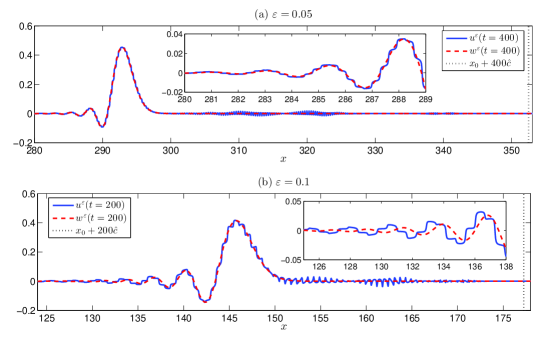
Figure 1: One-dimensional equation: the solutions $u^{\varepsilon}$ and $w^{\varepsilon}$ for $a_{Y}(y)=1.5+1.4\cos(y)$ and $f(x)=e^{-0.4x^{2}}$ are compared. Only the right propagating part of the solution is plotted. In (a) we have $\varepsilon=0.05$ and in (b) $\varepsilon=0.1$. The insets zoom in on the dispersive oscillations to the left of the main peak.

In Fig. 2 we study the convergence of the $L^{2}(\mathbb{R})-$error for the same material function and initial data as above. The error is computed at $\varepsilon=0.2,0.1$ and $0.05$ and $t=\varepsilon^{-2}$. The error values are approximately $0.1954,0.0977,0.0494$. Clearly, the numerical convergence is close to linear, in agreement with Theorem 1.2.

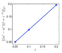
Figure 2: Convergence of the $L^{2}$-error $\|u^{\varepsilon}-w^{\varepsilon}\|_{L^{2}}$ at $t=\varepsilon^{-2}$ for $a_{Y}(y)=1.5+1.4\cos(y)$, $f(x)=e^{-0.4x^{2}}$, and the three values $\varepsilon=0.2$, $\varepsilon=0.1$, and $\varepsilon=0.05$. We emphasize that this is a severe test for convergence: in both steps, $\varepsilon$ is halved and the time instance is quadrupled.

4.2 Two space dimensions

Full two-dimensional ($n=2$) simulations for small values of $\varepsilon>0$ and time intervals of order $O(\varepsilon^{-2})$ are computationally expensive due to the need to discretize each period of size $O(\varepsilon)\times O(\varepsilon)$ in a domain of size $O(\varepsilon^{-2})\times O(\varepsilon^{-2})$. We therefore perform instead a simulation that is designed to mimic the long time behavior of a solution originating from localized initial data. After a long time the solution develops a large, close to circular, front. Within the strip

$$\Omega_{s}:=x\in\mathbb{R}\times(-\varepsilon\pi,\varepsilon\pi)$$

we can expect that the front is nearly periodic in the $x_{2}-$direction. Therefore, we perform tests on $\Omega_{s}$ with periodic boundary conditions in $x_{2}$, and initial data that are localized in $x_{1}$ and constant in $x_{2}$. Our choice is to take $f(x)=e^{-0.6x_{1}^{2}},\ x\in\Omega_{s}$. We select a material function that describes a smoothed square structure, namely

$$a_{Y}(y)= (1+c(y)-\overline{c})I,$$ (4.3)

$$\quad c(y)= \frac{1}{8}\prod_{j=1}^{2}\left[1+\tanh\left(4(y_{j}+\tfrac{3}{5}\pi)\right)\right]\left[1-\tanh\left(4(y_{j}-\tfrac{3}{5}\pi)\right)\right],$$

where $\overline{c}:=\tfrac{1}{|Y|}\int_{Y}c(y)dy$ and $I=\left(\begin{smallmatrix}1&0\\ 0&1\end{smallmatrix}\right)$. This choice ensures a relatively large value of the dispersive coefficient $\alpha$. We find

$$a^{*}\approx 0.5808,\quad\alpha\approx-0.3078,\quad\beta\approx 0.0515.$$

These values correspond to case 2 in Remark 3.2 so that $AD^{2}=a^{*}\Delta\approx 0.5808\,\Delta$, $ED^{2}=\tfrac{|\alpha|}{a^{*}}\Delta\approx 0.5300\,\Delta,$ $FD^{4}=(|\alpha|+3\beta)\partial_{x_{1}}^{2}\partial_{x_{2}}^{2}\approx 0.4623\,\partial_{x_{1}}^{2}\partial_{x_{2}}^{2}$. Due to the $x_{2}-$independence of the initial data, the solution of the effective model (1.5) on $\Omega_{s}$ stays constant in $x_{2}$ so that $FD^{4}$ can be dropped and (1.5) becomes

$$\partial_{t}^{2}w^{\varepsilon}=0.5808\,\partial_{x_{1}}^{2}w^{\varepsilon}+\varepsilon^{2}\,0.53\,\partial_{x_{1}}^{2}\partial_{t}^{2}w^{\varepsilon}.$$

In the simulations of (1.1) we use $\Delta x_{1}=\Delta x_{2}=2\pi\varepsilon/30$ and $\Delta t=0.004$, and in (1.5) we use $\Delta x_{1}=2\pi/100$ and $\Delta t=0.01$.

In Fig. 3 the main part of the right propagating half of the solution $u^{\varepsilon}$ is plotted for $\varepsilon=0.1$ at $t=100=\varepsilon^{-2}$. One clearly sees dispersive oscillations behind the main pulse.

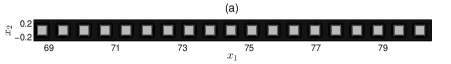
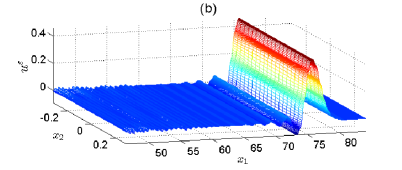
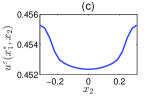
Figure 3: Two-dimensional equation: (a) The periodic structure $a^{\varepsilon}(x)$ given by (4.3) over a section of the strip $\Omega_{s}$. (b) The main part of the right propagating part of the solution $u^{\varepsilon}$ at $t=100$ for $\varepsilon=0.1$ and $f(x)=e^{-0.6x_{1}^{2}}$. (c) The $x_{2}$-profile of $u^{\varepsilon}$ at $x_{1}=x_{1}^{*}$ with $x_{1}^{*}$ being the position of the peak of the pulse.

Fig. 4 shows the agreement between $w^{\varepsilon}$ and the $x_{2}-$mean of $u^{\varepsilon}$ at $\varepsilon=0.1$ and $t=\varepsilon^{-2}$.

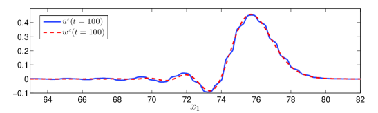
Figure 4: Comparison of $\bar{u}^{\varepsilon}(x_{1},t):=\tfrac{\varepsilon}{2\pi}\int_{-\varepsilon\pi}^{\varepsilon\pi}u^{\varepsilon}(x_{1},x_{2},t)dx_{2}$ and $w^{\varepsilon}$ at $\varepsilon=0.1$ and $t=\varepsilon^{-2}$ for $a^{\varepsilon}(x)$ given by (4.3) and $f(x)=e^{-0.6x^{2}}$.

Conclusions

We have performed an analysis of wave propagation in multi-dimensional heterogeneous media (periodic with length-scale $\varepsilon>0$). It is well-known that for large times, solutions cannot be approximated well by the homogenized second order wave equation. We have provided here a suitable well-posed dispersive wave equation of fourth order that describes the original solution $u^{\varepsilon}$ on time intervals of order $O(\varepsilon^{-2})$. Our analytical results provide an error estimate of order $O(\varepsilon)$ between $u^{\varepsilon}$ and the solution $w^{\varepsilon}$ of the dispersive equation. The coefficients of the effective equation are computable from the dispersion relation, which, in turn, is given by eigenvalues of a cell-problem. The qualitative agreement between $u^{\varepsilon}$ and $w^{\varepsilon}$ is confirmed by one-dimensional numerical tests, that even provide a confirmation of the linear convergence of the error in $\varepsilon$. In two space dimensions we can observe the validity of the dispersive equation in a simplified setting, computing solutions on a long strip.

Appendix A $H^{1}$-convergence of the Bloch expansion

Our aim here is to show that relation (2.8) holds as a convergence of the partial sums in $H^{1}(\mathbb{R}^{n})$. Since $\varepsilon>0$ is fixed, for brevity of notation we may as well conclude the $H^{1}(\mathbb{R}^{n})$-convergence in (2.3) for $g\in H^{2}(\Omega)$.

With the operator $L:=\nabla\cdot(a_{Y}(y)\nabla)$ we can expand the two $L^{2}(\mathbb{R}^{n})$-functions $g$ and $h=Lg$ in a Bloch series,

$$g =L^{2}(\mathbb{R}^{n})-\lim_{M\to\infty}g^{M}\quad\text{ for }\quad g^{M}(y):=\sum_{m=0}^{M}\int_{Z}\hat{g}_{m}(k)w_{m}(y,k)\,dk\,,$$

$$Lg=h =L^{2}(\mathbb{R}^{n})-\lim_{M\to\infty}h^{M}\quad\text{ for }\quad h^{M}(y):=\sum_{m=0}^{M}\int_{Z}\hat{h}_{m}(k)w_{m}(y,k)\,dk\,.$$

The formulas for $\hat{g}_{m}(k)$ and $\hat{h}_{m}(k)$ provide, by construction of $w_{m}$ as an eigenfunction of $L$ and the symmetry of $L$,

$$\hat{h}_{m}(k)=\int_{\mathbb{R}^{n}}(Lg)(y)w_{m}(y,k)^{*}\,dy=\int_{\mathbb{R}^{n}}g(y)Lw_{m}(y,k)^{*}\,dy=\mu_{m}(k)\hat{g}_{m}(k)\,.$$

In consequence, we obtain

$$Lg^{M}(y) =\sum_{m=0}^{M}\int_{Z}\hat{g}_{m}(k)\mu_{m}(k)w_{m}(y,k)\,dk=\sum_{m=0}^{M}\int_{Z}\hat{h}_{m}(k)w_{m}(y,k)\,dk=h^{M}(y)\,.$$

The right hand side converges in $L^{2}(\mathbb{R}^{n})$ to $h=Lg$. The elliptic operator $L$ allows to conclude from the $L^{2}(\mathbb{R}^{n})$-convergence $Lg^{M}\to Lg$ the $H^{1}(\mathbb{R}^{n})$-convergence $g^{M}\to g$.

Appendix B Variant of the Gronwall inequality

We provide now the proof of the Gronwall-type inequality (3.15). Let $Y:[0,T]\to[0,\infty)$ be a function such that, for a constant $Y_{0}\geq 0$, the relation

$$Y(t)\leq 2\int_{0}^{t}\|R(.,s)\|_{L^{2}(\mathbb{R}^{n})}\sqrt{Y(s)}\,ds+Y_{0}$$ (B.1)

holds for all times $t\in[0,T]$. We claim that then

$$Y(t)\leq 2\left(\int_{0}^{t}\|R(.,s)\|_{L^{2}(\mathbb{R}^{n})}\,ds\right)^{2}+2Y_{0}$$ (B.2)

holds for all times $t\in[0,T]$.

For the proof we define $Z(t)$ to be the integral on the right hand side of (B.1),

$$Z(t):=2\int_{0}^{t}\|R(.,s)\|_{L^{2}(\mathbb{R}^{n})}\sqrt{Y(s)}\,ds.$$

Then $Z(0)=0$ and, due to the assumption (B.1),

$$\frac{d}{dt}Z(t)=2\|R(.,t)\|_{L^{2}(\mathbb{R}^{n})}\sqrt{Y(t)}\leq 2\|R(.,t)\|_{L^{2}(\mathbb{R}^{n})}\sqrt{Z(t)+Y_{0}}\,.$$

We conclude that

$$\frac{d}{dt}\left(\sqrt{Z(t)+Y_{0}}\right)=\left(2\sqrt{Z(t)+Y_{0}}\right)^{-1}\frac{d}{dt}Z(t)\leq\|R(.,t)\|_{L^{2}(\mathbb{R}^{n})}.$$

Integrating this relation over $[0,t]$ we obtain, recalling $Z(0)=0$,

$$\sqrt{Z(t)+Y_{0}}-\sqrt{Y_{0}}\leq\int_{0}^{t}\|R(.,s)\|_{L^{2}(\mathbb{R}^{n})}\,ds\,.$$

By evaluating the square we find

$$Z(t)+Y_{0} \leq\left(\sqrt{Y_{0}}+\int_{0}^{t}\|R(.,s)\|_{L^{2}(\mathbb{R}^{n})}\,ds\right)^{2}$$

$$\leq 2Y_{0}+2\left(\int_{0}^{t}\|R(.,s)\|_{L^{2}(\mathbb{R}^{n})}\,ds\right)^{2},$$

and therefore the claimed result (B.2), since $Y(t)\leq Z(t)+Y_{0}$ holds by assumption.

References

- [1] A. Abdulle, M. J. Grote, and C. Stohrer. FE heterogeneous multiscale method for long-time wave propagation. C. R. Math. Acad. Sci. Paris, 351(11-12):495–499, 2013.
- [2] G. Allaire. Homogenization and two-scale convergence. SIAM J. Math. Anal., 23(6):1482–1518, 1992.
- [3] G. Allaire. Dispersive limits in the homogenization of the wave equation. Ann. Fac. Sci. Toulouse Math. (6), 12(4):415–431, 2003.
- [4] G. Allaire, C. Conca, and M. Vanninathan. The Bloch transform and applications. In Actes du 29ème Congrès d’Analyse Numérique: CANum’97 (Larnas, 1997), volume 3 of ESAIM Proc., pages 65–84 (electronic). Soc. Math. Appl. Indust., Paris, 1998.
- [5] G. Allaire, M. Palombaro, and J. Rauch. Diffractive behavior of the wave equation in periodic media: weak convergence analysis. Ann. Mat. Pura Appl. (4), 188(4):561–589, 2009.
- [6] S. Brahim-Otsmane, G. A. Francfort, and F. Murat. Correctors for the homogenization of the wave and heat equations. J. Math. Pures Appl. (9), 71(3):197–231, 1992.
- [7] C. Castro and E. Zuazua. Low frequency asymptotic analysis of a string with rapidly oscillating density. SIAM J. Appl. Math., 60(4):1205–1233 (electronic), 2000.
- [8] G. Cohen and P. Joly. Construction analysis of fourth-order finite difference schemes for the acoustic wave equation in nonhomogeneous media. SIAM J. Numer. Anal., 33(4):1266–1302, 1996.
- [9] C. Conca, R. Orive, and M. Vanninathan. Bloch approximation in homogenization and applications. SIAM J. Math. Anal., 33(5):1166–1198 (electronic), 2002.
- [10] C. Conca, R. Orive, and M. Vanninathan. On Burnett coefficients in periodic media. J. Math. Phys., 47(3):032902, 11, 2006.
- [11] C. Conca and M. Vanninathan. Homogenization of periodic structures via Bloch decomposition. SIAM J. Appl. Math., 57(6):1639–1659, 1997.
- [12] T. Dohnal and W. Dörfler. Coupled mode equation modeling for out-of-plane gap solitons in 2d photonic crystals. Multiscale Modeling & Simulation, 11(1):162–191, 2013.
- [13] T. Dohnal and H. Uecker. Coupled mode equations and gap solitons for the 2D Gross-Pitaevskii equation with a non-separable periodic potential. Phys. D, 238(9-10):860–879, 2009.
- [14] J. Fish and W. Chen. Space-time multiscale model for wave propagation in heterogeneous media. Comput. Methods Appl. Mech. Engrg., 193(45-47):4837–4856, 2004.
- [15] J. Fish, W. Chen, and G. Nagai. Uniformly valid multiple spatial-temporal scale modeling for wave prpagation in heterogeneous media. Mechanics of Composite Materials and Structures, 8:81–99, 2001.
- [16] J. Fish, W. Chen, and G. Nagai. Non-local dispersive model for wave propagation in heterogeneous media: multi-dimensional case. Internat. J. Numer. Methods Engrg., 54(3):347–363, 2002.
- [17] J. Fish, W. Chen, and G. Nagai. Non-local dispersive model for wave propagation in heterogeneous media: one-dimensional case. Internat. J. Numer. Methods Engrg., 54(3):331–346, 2002.
- [18] G. A. Francfort and F. Murat. Oscillations and energy densities in the wave equation. Comm. Partial Differential Equations, 17(11-12):1785–1865, 1992.
- [19] J. Francu and P. Krejčí. Homogenization of scalar wave equations with hysteresis. Contin. Mech. Thermodyn., 11(6):371–390, 1999.
- [20] A. Lamacz. Dispersive effective models for waves in heterogeneous media. Math. Models Methods Appl. Sci., 21(9):1871–1899, 2011.
- [21] A. Lamacz. Waves in heterogeneous media: Long time behavior and dispersive models. PhD thesis, TU Dortmund, 2011.
- [22] G. Lebeau. The wave equation with oscillating density: observability at low frequency. ESAIM Control Optim. Calc. Var., 5:219–258 (electronic), 2000.
- [23] R. Orive, E. Zuazua, and A. F. Pazoto. Asymptotic expansion for damped wave equations with periodic coefficients. Math. Models Methods Appl. Sci., 11(7):1285–1310, 2001.
- [24] M. Reed and B. Simon. Methods of modern mathematical physics. IV. Analysis of operators. Academic Press, New York, 1978.
- [25] E. Sánchez-Palencia. Nonhomogeneous media and vibration theory, volume 127 of Lecture Notes in Physics. Springer-Verlag, Berlin, 1980.
- [26] F. Santosa and W. W. Symes. A dispersive effective medium for wave propagation in periodic composites. SIAM J. Appl. Math., 51(4):984–1005, 1991.
- [27] B. Schweizer. Homogenization of the Prager model in one-dimensional plasticity. Contin. Mech. Thermodyn., 20(8):459–477, 2009.
- [28] B. Schweizer and M. Veneroni. Periodic homogenization of the Prandtl–Reuss model with hardening. Journal of Multiscale Modelling, 02(01n02):69–106, 2010.
- [29] C. H. Wilcox. Theory of Bloch waves. J. Analyse Math., 33:146–167, 1978.