Ab Initio Equation of State for Hydrogen-Helium Mixtures with Recalibration of the Giant-Planet Mass-Radius Relation

Abstract

Using density functional molecular dynamics simulations, we determine the equation of state for hydrogen-helium mixtures spanning density-temperature conditions typical of giant planet interiors, $\sim$ 0.2$-$9 g cm^-3 and 1000$-$80 000 K for a typical helium mass fraction of 0.245. In addition to computing internal energy and pressure, we determine the entropy using an ab initio thermodynamic integration technique. A comprehensive equation of state (EOS) table with 391 density-temperature points is constructed and the results are presented in form of two-dimensional free energy fit for interpolation. Deviations between our ab initio EOS and the semi-analytical EOS model by Saumon and Chabrier are analyzed in detail, and we use the results for initial revision of the inferred thermal state of giant planets with known values for mass and radius. Changes are most pronounced for planets in the Jupiter mass range and below. We present a revision to the mass-radius relationship which makes the hottest exoplanets increase in radius by $\sim$ 0.2 Jupiter radii at fixed entropy and for masses greater than $\sim$ 0.5 Jupiter mass. This change is large enough to have possible implications for some discrepant “inflated giant exoplanets”.

1 Introduction

The semi-analytical model by Saumon & Chabrier (1992) (SC) for the EOS of hydrogen and its extension to hydrogen-helium mixtures (Saumon et al., 1995) were very successful and have been used in numerous calculations for the interiors of giant planets. However, with the development of ab initio computer simulation techniques many uncontrolled approximations can now be avoided, simplifications inherent to analytical EOS models and severely limiting their predictive capabilities in the regime of high density and low temperature where interactions between particles are strong. Relying solely on analytical methods, it is difficult to determine the ionization state of the different chemical species that are present in the dense fluid.

Ab initio simulations allow one to study a fully interacting system of particles and to determine its properties by deriving the electronic states explicitly for every configuration of nuclei. No parameters are adjusted to match experimental data, but ab initio simulations still rely on approximations to solve the Schrödinger equation. However, they are not specific to the particular material nor the pressure-temperature conditions under consideration.

In this paper, we rely on density functional molecular dynamics (DFT-MD) simulations that have been employed before to study hydrogen (Lenosky et al., 2000; Militzer et al., 2001; Desjarlais, 2003; Bonev et al., 2004; Nettelmann et al., 2008; Morales et al., 2010; Caillabet et al., 2011; Collins et al., 2012; Nettelmann et al., 2012), helium (Militzer, 2006; Stixrude & Jeanloz, 2008; Militzer, 2009) and hydrogen-helium mixtures (Vorberger et al., 2007b, a; Militzer et al., 2008; Militzer, 2009; Hamel et al., 2011). While the computation of the pressure and the internal energy is straightforward from DFT-MD simulations, the entropy is not directly accessible. However, an accurate knowledge of the entropy of hydrogen-helium mixtures at high pressure is of crucial importance for the determination of the temperature profile, the density, and the thermal energy budget in the interior of a giant planet. In 2008, two groups constructed Jupiter interior models from DFT-MD simulations (Militzer et al., 2008; Nettelmann et al., 2008). While the derived pressures and internal energies can be considered to be more reliable than those predicted by the SC model, both papers predicted very different interior temperature profiles for Jupiter (Militzer & Hubbard, 2009). Using ab initio thermodynamic integration techniques (TDI), we recently showed (Militzer, 2013), that the work by Nettelmann et al. (2008) overestimated the temperature at Jupiter’s core-mantle boundary (CMB) by 3050 K (19%) while we underestimated it by 2870 K (18%) in Militzer et al. (2008). The revised temperature for the Jupiter’s CMB is 16 150 K and the corrections to the SC EOS model are in fact only $-350\,$K.

At conditions of Jupiter’s CMB, hydrogen is metallic and characterized by a high degree of electronic degeneracy. Such a degenerate state is described rather well by the the SC model. However, when we applied the TDI technique to explicitly determine the entropy over a wide range of pressure-temperature conditions, we identified a number of discrepancies between the DFT-MD results and the SC model. Near the molecular-to-metallic transition, our simulations predict a significant shift of the adiabat towards higher densities. At high temperature, where electronic excitations matter, our computed entropies are higher than those of the SC model. We also do not perfectly reproduce the SC entropies in the molecular regime at low density.

Rather than providing a separate hydrogen and helium EOS and relying on the linear mixing approximation (Saumon et al., 1995; Nettelmann et al., 2008), we computed the EOS over a wide range of density-temperature conditions for a representative mixing ratio of $N_{\rm He}=$18 helium atoms in $N_{\rm H}=220$ hydrogen atoms, corresponding to a helium mass fraction of $Y$=0.245, which is close to the solar value. This means that the nonideal mixing effects are fully incorporated. In Vorberger et al. (2007b), we showed for example that the presence of helium makes the hydrogen molecules more stable and reduces the dissociation fraction at given pressure and temperature. Even if other mixing ratios become of interest, as the result of helium rain (Stevenson & Salpeter, 1977; Morales et al., 2009; Wilson & Militzer, 2010; McMahon et al., 2012), one is still better off by starting from an EOS for a typical hydrogen-helium mixture and then perturbing the mixing ratio by a comparatively small amount. Increasing or decreasing the helium fraction requires knowledge of a helium or hydrogen EOS, respectively. For the helium EOS, we recommend our first-principles computation (Militzer, 2009) because it provides simulation data points for the pressure, $P$, internal energy, $E$, Helmholtz free energy, $F$, and entropy, $S$, over a wide parameter range and a thermodynamically consistent free energy fit for interpolation. For available hydrogen EOS work, we refer to the recent review by  McMahon et al. (2012) but there has also been a considerable theoretical effort compute the hydrogen EOS with semi-analytical techniques (Dharma-wardana & Perrot, 2002; Kraeft et al., 2002; Rogers & Nayfonov, 2002; Safa & Pfenniger, 2008; Ebeling et al., 2012; Alastuey & Ballenegger, 2012). If the perturbation in the helium fraction is sufficiently small, one may use the SC EOS for simplicity.

2 Ab Initio Simulations

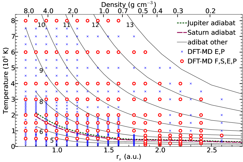
Figure 1: Temperature-density conditions of DFT-MD simulations. The circles indicate parameters where entropy and free energy have been calculated in addition to the pressure and internal energy. The lines show adiabats. The labels specify their entropy values in units of $k_{b}$ per electron.

We base our ab initio entropy calculations on our recent article (Militzer, 2013) where we showed how the TDI technique can be extended to study molecular hydrogen and how it can be applied efficiently to determine the entropy at high temperature where electronic excitations matter. The TDI technique allows one to determine the difference in the Helmholtz free energy between two interacting many-body systems at fixed density and temperature (Morales et al., 2009; Wilson & Militzer, 2010, 2012a, 2012b; McMahon et al., 2012). We apply this method to determine the free energy difference between the DFT simulations and a system of classical forces that we construct:

$$F_{\rm DFT}-F_{\rm cl}=\int_{0}^{1}d\lambda\;\left<V_{\rm KS}-V_{\rm cl}\right>_{\lambda}.$$ (1)

The angle brackets represent an average over trajectories governed by forces that are derived from a hybrid potential energy function, $V_{\lambda}=\lambda V_{\rm KS}+(1-\lambda)V_{\rm cl}$. $V_{\rm cl}$ is the potential energy of the classical system and $V_{\rm KS}$ is the Kohn-Sham energy (Kohn & Sham, 1965). The presence of electronic excitations leads to an intrinsic contribution to the entropy and affects the forces on the nuclei (de Wijs et al., 1998) that need to be derived from the Mermin free energy (Mermin, 1965), $\Omega=V_{\rm KS}-TS_{\rm el}$. We combined both contributions into the following expression for the ab initio entropy (Militzer, 2013):

$$TS=\left<V_{\rm KS}\right>+\left<K_{\rm ion}\right>-\int_{0}^{1}d\lambda\;\left<\Omega-V_{\rm cl}\right>_{\lambda}-F_{\rm cl}.$$ (2)

$\left<V_{\rm KS}\right>$ includes contributions from partially occupied excited states. The $\lambda$ integration was performed using five independent MD simulations with $\lambda$ equally spaced between 0 and 1. To make this integration process efficient, we construct the pair potentials of the classical system to match the DFT forces as closely as possible (Izvekov et al., 2003). The computation of classical free energy is performed with Monte Carlo methods by thermodynamic integration to an system of noninteracting particles.

All simulations were performed with the VASP code (Kresse & Furthmüller, 1996) with pseudopotentials of the projector-augmented wave type (Blöchl, 1994) and a plane wave basis set cutoff of at least 1000 eV. The Perdew-Burke-Ernzerhof exchange-correlation functional (Perdew et al., 1996) was used throughout, but it has been shown recently that simulations based on the local density approximation yielded very similar results for Jupiter’s deep interior (Militzer, 2013). In the same article, we also performed a combined finite-size and $k$ point analysis that demonstrated that simulations with 256 electrons and the zone-average point $k=(\frac{1}{4},\frac{1}{4},\frac{1}{4})$ are sufficiently accurate. All results that we report in this article were thus obtained with 220 hydrogen and 18 helium atoms in periodic boundary conditions.

We used a MD time step 0.2 fs, except for temperature of 50 000 K and above where we used a time step of 0.1 fs to accurately capture the more rapid collisions between particles at elevated temperatures. All standard DFT-MD simulations that we performed to determine $P$ and $E$ were 2.0 ps long, except at the highest temperatures, where 1.0 ps were found to be sufficient because the auto-correlation times are short and the error bars are small. All simulations were initialized with positions and velocity vectors from converged MD simulations at nearby densities and temperatures. This allowed us to run the TDI simulations for only 0.5 ps at each $\lambda$ point.

We also adjusted the number of orbitals in the calculations to accommodate the partial occupation of excited electronic states according to Mermin functional (Mermin, 1965). The number of orbitals was increased until the error in the integral of the Fermi function was reduced to less than 10^-5. This required many orbitals at high temperature and low density. Up to 816 were used, a significant increase in the computational cost over the 128 needed for ground state calculations. This is the primary reason why we omitted simulations that would lead to entropy values above approximately 12.5 $k_{b}$/el. The regime of higher temperatures can be studied much more efficiently with path integral Monte Carlo (PIMC) simulations because the computational cost of this alternative first-principles simulation technique scales like $1/T$. PIMC simulations have been applied to hydrogen (Pierleoni et al., 1994; Magro et al., 1996; Militzer et al., 1999; Militzer & Ceperley, 2000; Militzer & Graham, 2006; Hu et al., 2010, 2011), helium (Militzer, 2006, 2009), and hydrogen-helium mixtures (Militzer, 2005) at high pressure and temperature and most recently also to study the EOS of carbon and water (Driver & Militzer, 2012).

3 Equation of State Results

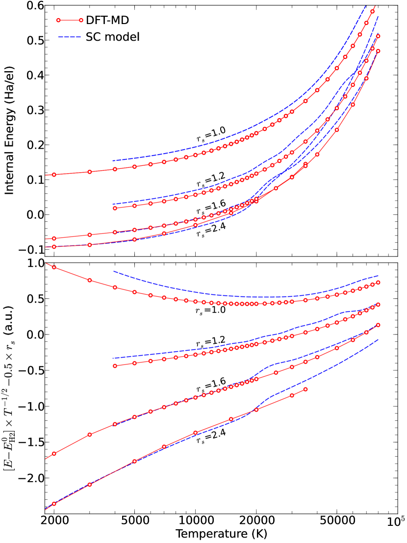
Figure 2: Internal energy per electron as function of temperature for four different densities given in terms of $r_{s}$. Results from DFT-MD simulations are compared with the analytical SC model.

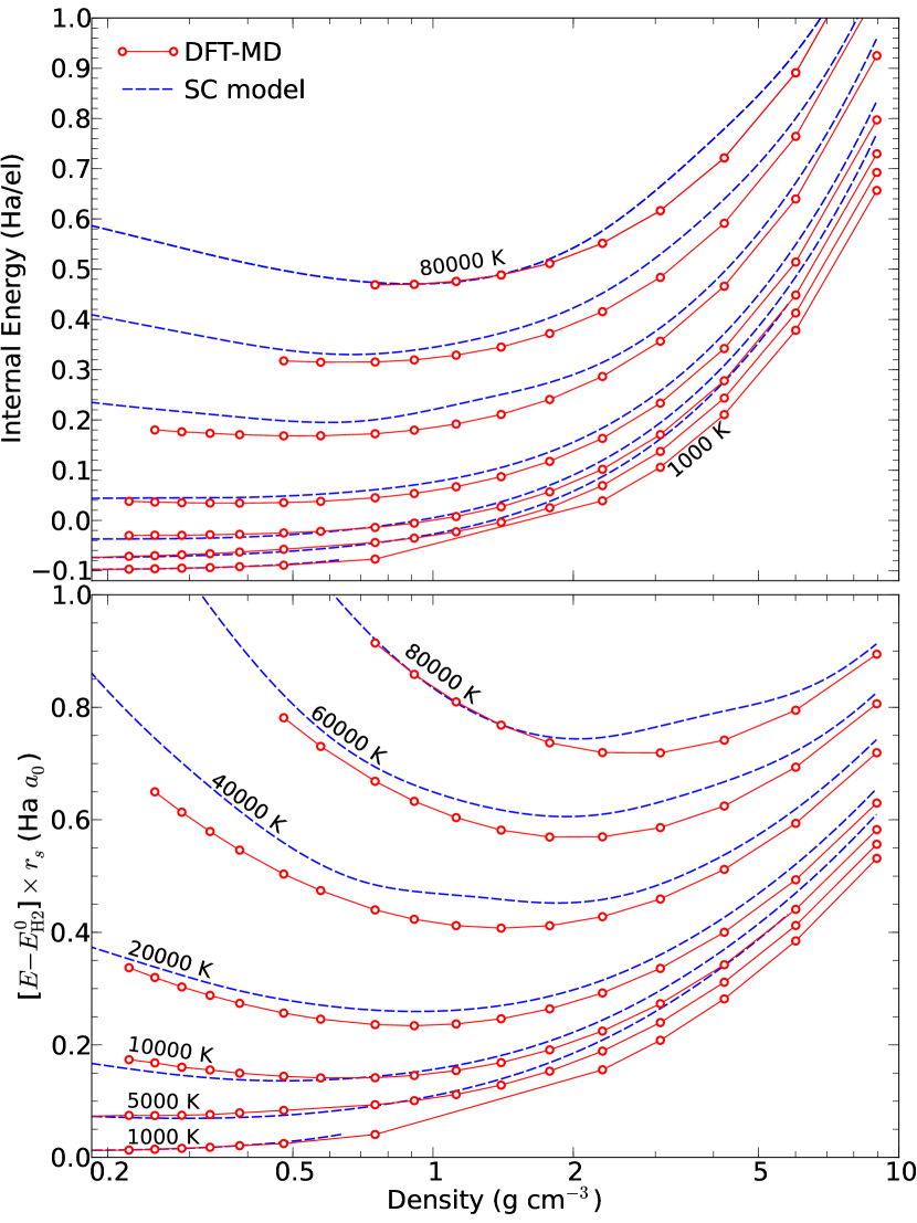
Figure 3: Internal energy per electron as function of density for seven different temperatures. Predictions from DFT-MD simulations and from the analytical SC EOS model are compared.

We report the computed equation of state in the form of a table, a series of figures, and in analytical form as two-dimensional fit of the free energy. In table 1, we provide the thermodynamic functions that directly follow from analysis of the DFT-MD trajectories. The pressure and internal energy were computed for 391 different density-temperature points (see Fig. 1). The 1-$\sigma$ error bars correspond to statistical uncertainty that arises from the finite length of the MD simulations. For 131 points in table 1, the thermodynamic integration was performed with five $\lambda$ points and the free energy and entropy are reported in addition. Only counting the production runs that led to results in table 1, the total CPU time consumed for this project amounted to 850 000 core-hours on Intel Nehalem processors. This is equivalent to using 100 cores for an entire year, which is a considerable amount of computer time by today’s standards but will certainly become available to everyone in the near future as computers with more and more cores are assembled.

In figures 2, 3, 4, 5, 6, 7, 8, and 9, we plot the internal energy, pressure, Helmholtz free energy, and entropy respectively as a function of temperature and density. Every circle corresponds to a particular DFT-MD simulation listed in table 1, without any interpolation being performed. The dashed lines are the results of the most common version of the analytical SC EOS model where the different thermodynamic functions have been smoothly interpolated across the molecular-to-metallic transition in hydrogen.

To accommodate the wide parameter range of our simulations, we plot the different thermodynamic functions on logarithmic scale. Since these functions depend strongly on density and temperature, we added a second panel where we removed most of this dependence by introducing a scale factor equal to $r_{s}$ or $T$ raised to some power. Here $r_{s}$ is the Wigner-Seitz radius that specifies the density of system according to $\frac{4\pi}{3}r_{s}^{3}=V/N_{e}=n^{-1}$, while $n$ is the number of electrons, $N_{e}=(N_{\rm H}+2N_{\rm He})$, per unit volume $V$. The mass density is given by $\rho=n(N_{\rm H}m_{\rm H}+N_{\rm He}m_{\rm He})/(N_{\rm H}+2N_{\rm He})$ where $m_{\rm H}$ and $m_{\rm He}$ are the masses of the hydrogen and helium atoms.

The rescaling of the ordinate makes it easier to identify the deviations from the SC model while our simulation results can still be reproduced easily. The ordinates are plotted in atomic units. Lengths including $r_{s}$ are given in Bohr radii ($a_{0}$=5.29177209$\times 10^{-11}\,$m), energies in Hartrees (4.35974380$\times 10^{-18}\,$J) per electron (el.), and entropies are specified in units of $k_{b}$ per electron, where $k_{b}$ is Boltzmann’s constant.

Figure 2 shows a comparison between the internal energies from DFT-MD simulations with the predictions of the SC EOS model. For a low density of $r_{s}=2.4$, excellent agreement is found for a temperature range from 1000 to 20 000 K. Hydrogen gradually changes from a molecular state to an atomic state in this temperature interval and, from the good agreement, one may conclude that the thermally activated dissociation of molecules is well described in the SC model. However, 20 000 K, the SC model predicts an strong and artificial increase in the internal energy that is the result of an inaccurate description of electronic excitations. This deviation was first identified by Militzer & Ceperley (2001) when predictions from the SC model were compared with PIMC simulations. Figure 3 shows that this deviation is present at 20 000 K for whole density range under consideration and extends to much higher temperatures also.

Figure 2 shows that the favorable agreement between DFT-MD results and SC predictions below 20 000 K continues to hold up to a density of $r_{s}=1.6$. When the internal energy is compared for a higher density of $r_{s}=1.0$ or 1.2 where hydrogen is metallic, one finds that DFT-MD results and SC predictions are offset by a nearly constant amount.

The internal energy curves of $r_{s}=1.6$ and 2.4 appear to cross over in Fig. 2 at a temperature of 27 000 K, which is consistently predicted by DFT-MD results and the SC model. Figure 3 shows that this is simply a consequence of internal energy exhibiting a minimum when plotted at constant temperature as function of density. At high density, the internal energy sharply rises because of Pauli exclusion effects between the electrons. In the low density limit, the internal energy rises also because the ionization fraction increases as a result of the increased gain in entropy that is associated with electrons becoming free particles.

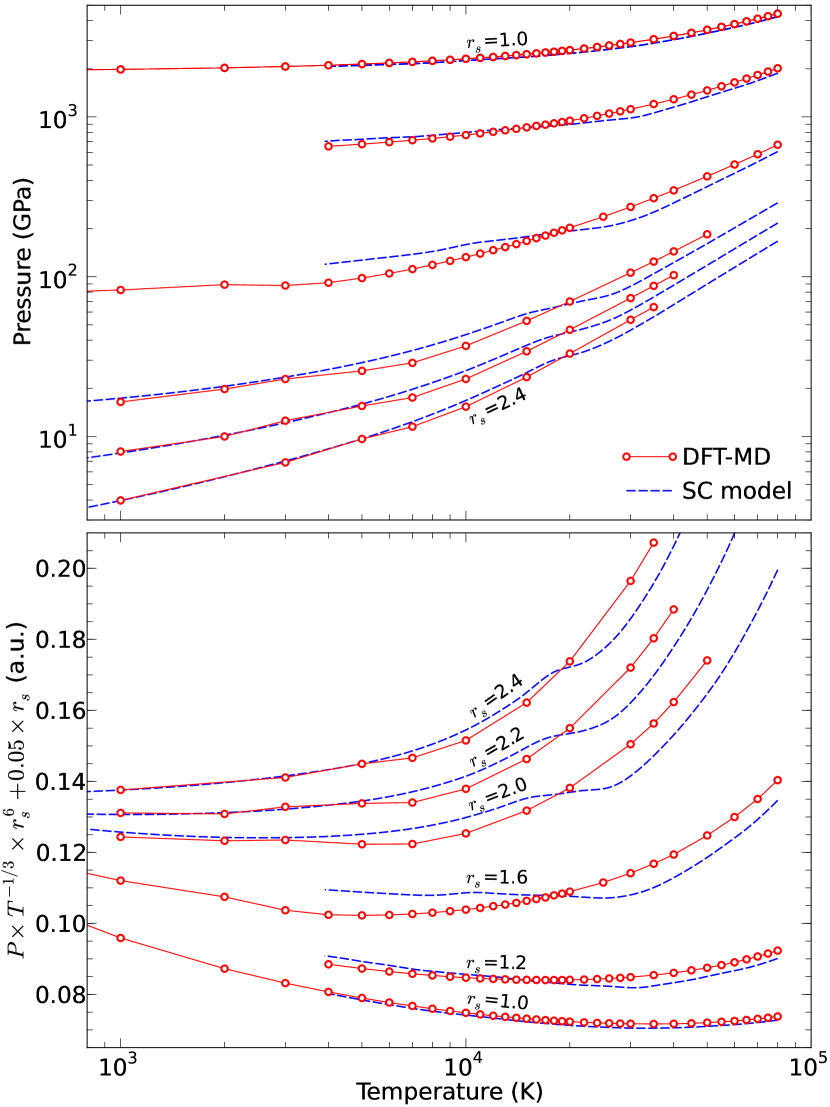
Figure 4: Pressure isochores computed with DFT-MD simulations are compared with the analytical SC model.

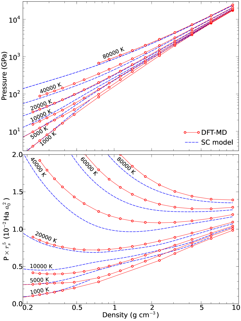
Figure 5: Pressure isotherms computed with DFT-MD simulations are compared with the analytical SC model.

In Fig. 4, we compare the pressure predicted from DFT-MD simulation with the SC model. At a high density of $r_{s}=1.0$ where the hydrogen-helium mixture is metallic, we find fairly good agreement over the entire temperature range. This implies that the deviation that we identified for the internal energy in this regime, varies slowly with density and does not significantly affect the pressure in the SC model.

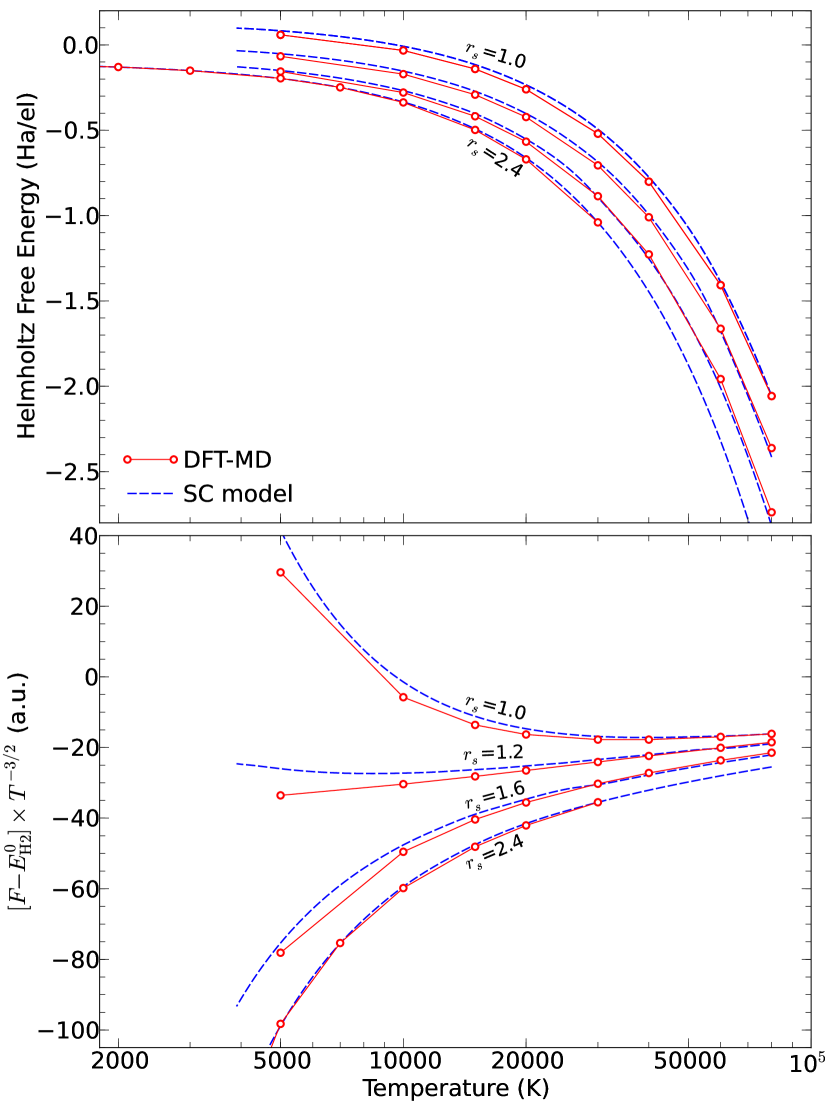
Figure 6: Helmholtz free energy per electron at constant density computed with DFT-MD simulations are compared with the analytical SC model.

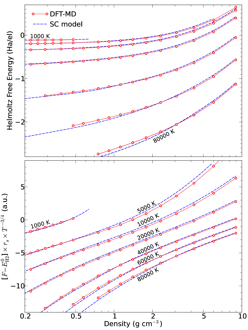
Figure 7: Helmholtz free energy per electron at constant temperature computed with DFT-MD simulations are compared with the analytical SC model.

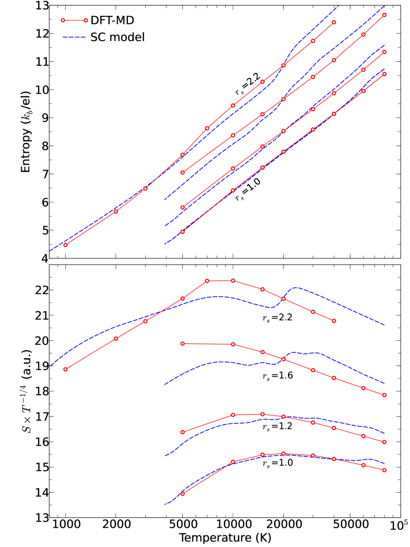
Figure 8: Entropy per electron at constant density computed with DFT-MD simulations are compared with the analytical SC model.

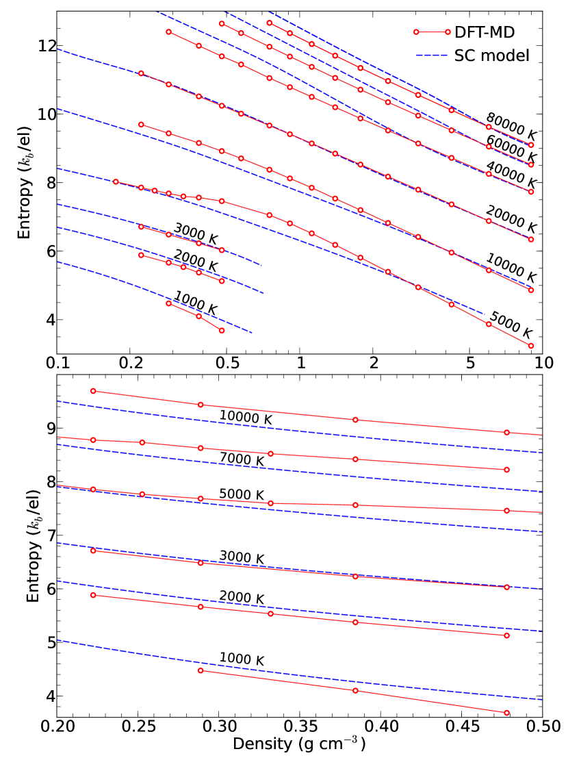
Figure 9: Entropy per electron at constant temperature computed with DFT-MD simulations are compared with the analytical SC model. The upper panel shows results over a wide temperature-density range while the lower panel zooms in on the low density regime where hydrogen occurs in molecular form when the temperature is below 5000 K.

At a low density of $r_{s}=2.2$ and 2.4, we found good agreement up to a temperature of 5000 K. At this temperature, we see a small decrease in slope in the DFT-MD data that is missing in the predictions of the SC model. We attribute this slope change to the dissociation of molecules in the DFT-MD simulations. At 20 000 K, the SC model predicts a significant decrease in slope which is not present in the DFT-MD data. This slope change in the SC predictions can again be attributed to an inaccurate description of ionization, which leads to deviations over the whole density range under consideration (Fig. 5). At an intermediate density of $r_{s}=1.6$ close to the molecular-to-metallic transition, we find that the SC model overestimates the pressure up to about 20 000 K and underestimates for higher temperatures. The deviations around 100 GPa, 5000 K, and $r_{s}=1.6$ (0.75 g cm^-3) are of particular significance. The DFT-MD simulations predict pressures that are much lower than those of the SC model. This leads a significant departure in the resulting adiabats. Its implication for the interiors of giant planets will later be further analyzed.

In figures 6 and 7, the Helmholtz free energy from DFT-MD simulations and the SC model are compared. In general the agreement appears to be much better than for other thermodynamic functions that are derivatives of it. Still, one finds that the SC model overestimates the free energy in the metallic regime, mirroring the deviations that we have discussed for the internal energy.

In figures 8, the entropies at different densities are compared as a function of temperature. At a very high density of $r_{s}=1.0$, very good agreement between DFT-MD results and the SC model is found up to 50 000 K. For lower densities, the SC model predicts a sharp entropy increase at 20 000 K, which is again a result of the treatment of ionization effects. This trend is not confirmed by the DFT-MD simulations. One also finds significant deviations at lower temperatures, in particular around $r_{s}$=1.6. Even at a relatively low density of $r_{s}=2.2$, the agreement is not perfect. From 4000 to 20 000 K, the SC model underestimates the entropy and it overestimates the entropy for lower temperatures. Figure 9 shows that such deviations persist over a wider density range. In principle, one expects a non- or weakly interacting gas of hydrogen molecules and helium atoms to be perfectly described by the SC model. However, the density that we can efficiently study with DFT-MD simulations does not yet appear to be low enough for the deviations to decay to zero.

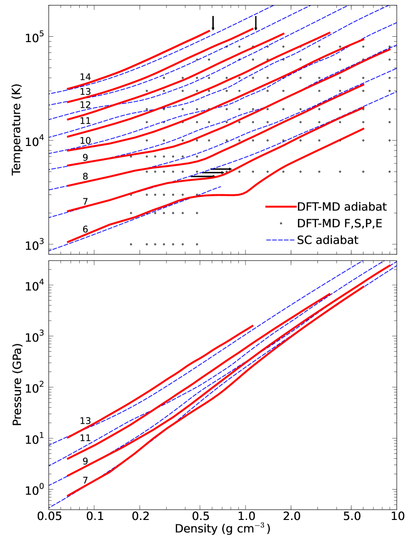
Figure 10: Adiabats derived from DFT-MD simulations are compared with the SC model. The labels denote the entropy in units of $k_{b}$ per electron. The circles indicate parameters where entropy and free energy have been calculated in addition to the pressure and internal energy. The horizontal arrows label conditions where the deviation from the SC model are large and important for the interiors of Saturn and Jupiter. The vertical arrows indicate deviations are high temperature where the SC model does not treat electronic excitations accurately.

4 Free Energy Fit for the Equation of State

We fitted our ab initio results for $P$, $E$, $F$, and $S$ in table 1 with a two-dimensional spline function that represents the Helmholtz free energy in terms of temperature, $T$, and electron density, $n=N_{e}/V$. By construction, this fit is thermodynamically consistent. We employ the same functional form that we used to represent the free energy of hot, dense helium in (Militzer, 2009), except the splines here are functions of $n$ rather than $\log(n)$. Table 2 provides the free energy as well as the required derivatives on a number of $(n,T)$ knot points. Atomic units are used throughout.

To evaluate the fit for $(n^{*},T^{*})$, we first construct a separate one-dimensional cubic spline function, $F_{n}(T)$, for every density on a grid ranging from $r_{s}$=3.581 to 0.536 (0.0670$-$20.0 g cm^-3). At every density, the free energy is given on a number of temperature knots and its first derivative, $\left.\frac{\partial F}{\partial T}\right|_{n}$, is specified for the highest and lowest temperatures. We construct a similar one-dimensional spline function that represents $\left.\frac{\partial F}{\partial n}\right|_{T}(T)$ at the smallest and largest density. We then evaluate all these splines functions at $T^{*}$ and construct a one-dimensional spline function $F_{T^{*}}(n)$ from the free energy values and its first derivatives at the boundaries. This provides us not only with a straightforward way to obtain the free energy at every $(n,T)$ point but we can also derive the pressure and entropy by taking analytical derivatives,

$$P=n^{2}\left.\frac{\partial F}{\partial n}\right|_{T}\;\;{\rm and}\;\;S=-\left.\frac{\partial F}{\partial T}\right|_{n}\;\;.$$ (3)

The internal energy and Gibbs free energy then follow from $E=F+TS$ and $G=F+PV$.

When we constructed this fit, we made sure every EOS point in table 1 is well reproduced. We extended the domain of the fit a bit beyond the range of the DFT-MD data. This leads to a smoother representation of the data in the interior of the domain and also allows us to gradually approach the SC EOS in the limit of low density. As figure 10 shows, we were able to smoothly match onto the SC adiabats for entropy values from 6 to 10 and again for 13 and 14 $k_{b}$/el. A disagreement remains for S=11 and 12 $k_{b}$/el. but the SC EOS is not thermodynamically consistent in the regime of 10 000  to 20 000 K and no attempt was made to reproduce those adiabats. So far, only the one exoplanet HAT-P-32b  (Hartman et al., 2011) appears to have an internal entropy in excess of 11 $k_{b}$/el.; see Figure 12.

We also find a significant disagreement in the high density limit between our DFT-MD adiabats and the predictions of the SC model. Starting with entropy values of $S=10\,k_{b}$/el., the DFT-MD results predict the adiabats reach states of higher temperatures and higher pressure for a given density.

The most significant result of Fig. 10 is the deviations along the $S$=7 $k_{b}$/el. adiabat. The DFT-MD simulations predict a decrease in slope of the adiabat exactly where the hydrogen molecules dissociate (Militzer et al., 2008). Since the SC model interpolates between separate atomic/metallic and molecular thermodynamic descriptions, it has no predictive power in the regime of pressure dissociation where all the different species interact strongly.

5 Giant Planet Interiors

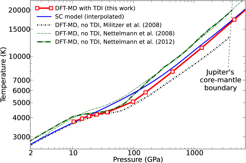
Figure 11: Adiabats from different calculations for Jupiter’s interior.

In Fig. 11, we compare different predictions for the adiabat in Jupiter’s interior. Similar to Militzer et al. (2008), the calculations of the entropy by Nettelmann et al. (2008, 2012) relied solely on the $P$ and $E$ from DFT-MD simulations. Since no TDI was employed, the entropy was determined indirectly from thermodynamic relationships and an integration over a large path through density-temperature space. Here one faces two challenges. Since the integration can only yield the entropy difference between two $\rho$-$T$ points, one needs to find a starting point for the integration where DFT-MD simulations work and the entropy is known reliably through other means. Secondly, one needs to determine $P$ and $E$ on a very fine grid in $\rho$-$T$ space, so that integration errors do not accumulate. Since both challenges are difficult to meet, we instead adopted the more reliable TDI technique that we extended to molecular systems in Militzer (2013).

Figure 11 shows that there exist some discrepancies between our TDI calculations and the Nettelmann et al. (2008, 2012) results in the low density as well as the high density limit. In the molecular regime at 10 GPa, Nettelmann et al.’s temperatures for Jupiter’s adiabat are 8% higher than our TDI calculations predict. In the metallic regime at 4000 GPa, their results are 19% higher than our TDI predictions. This implies that there exist discrepancies in the low and high density limits before any ab initio $P$ and $E$ data points are entered into the calculation of the adiabats by Nettelmann et al. (2008, 2012).

Adiabats based on the  Nettelmann et al. (2012) work now show a pronounced flattening in the regime of molecular dissociation from 15-40 GPa that was not present in the  Nettelmann et al. (2008) calculations. The pressure range similar to our ab initio results but the magnitude is higher than we predict based on TDI. From 40 to 200 GPa, the Nettelmann et al. (2012) calculations predict a steep rise in temperature for the adiabats. This is not consistent with our TDI calculations and implies that in models by  Nettelmann et al. (2012) most of Jupiter’s mass is at 19% higher temperature than we predict based on our TDI calculations. In the low and high density limits, our adiabats are instead in relatively good agreement with the SC model.

6 Mass-Radius Relationships

The vexing problem of radius anomalies of transiting giant planets  (Burrows et al., 2007) has continued with the addition of more objects  (Laughlin et al., 2011). Figure 12 shows measurements posted in the online Exoplanet Encyclopaedia (Schneider et al., 2011) as of late 2012 and different theoretical curves that we will discuss below. Briefly, the problem arises from a significant population of exoplanets that have radii too large to be explained by thermal distention from retained primordial heat, and there is a further population with radii well below those expected for primarily H-He composition even at zero temperature. Any point that falls below the $S=6\,k_{b}$/el. curve can be explained by invoking the presence of a rocky core and/or admixture of heavy elements, which reduces the radius for given mass (Miller & Fortney, 2011). But it is not so simple to classify the population of anomalously distended giant exoplanets, for the degree of distention depends on such factors as the planet’s age and degree of irradiation from the host star (Fortney & Nettelmann, 2010), and possible additional heating mechanisms such as ohmic dissipation (Batygin et al., 2011).

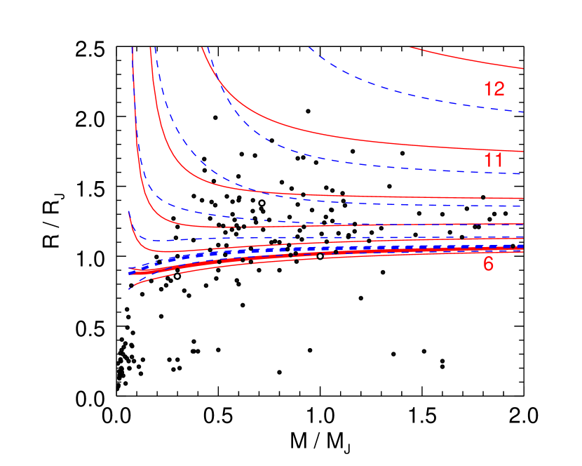
Figure 12: Radius $R$ (in units of $R_{J}=70000$ km vs. mass $M$ (in units of $M_{J}=$ Jupiter’s mass). The solid data points are measurements of transiting exoplanets. The curves show the $R(M)$ relation predicted from two EOS calculations (solid curves are for DFT-MD simulations, dashed curves are for the SC model) for fixed entropies of $S=$ 6, 6.8 (Saturn; heavy curve), 7 (Jupiter), 8, 9, 10, 11, and 12 $k_{b}$/el. The three open data points denote Saturn, HD 209458b, and Jupiter from left to right.

In order to most clearly exhibit the differences in predicted radius between the DFT-MD simulations and analytical SC model, we model a planet of mass $M$ as a H-He object of constant entropy $S$ and fixed helium fraction of $Y=0.245$ with neither a rocky core nor heavy element component in the gas envelope. Since we do not have DFT-MD simulation data at very low densities, we switch back to the SC model below 0.0670 g cm^-3, the lowest density of the free energy fit to our DFT-MD data.

As is well known (Chandrasekhar, 1957), formally such an object has a precisely defined radius where the temperature $T$, mass density $\rho$, and pressure $P$ simultaneously go to zero. In a real object, the ideal-gas outer layers cannot persist in such an isentropic state and instead the temperature reaches a finite limit set by the effective temperature for the radiation balance in the outer layers. The radius as measured by transit observations also depends on sources of slant opacity in these outer layers. As explored by Burrows et al. (2007), the value of such a radius can vary by several $0.1\,R_{J}$, depending on the atmospheric model. Adjusting the parameters controlling the atmosphere can move a model closer to agreement with objects of inflated radii, but sometimes a mismatch remains. A major result of the present paper is that differences in the EOS alone can also lead to radius changes of several $0.1\,R_{J}$. Because we consider only strict-adiabatic models, the deviations that we point out are entirely due to differences in the EOS at high pressure. In Figure 13, we exhibit these differences for various entropies. For entropy values up to 9 $k_{b}$/el., the DFT-MD calculations consistently predict smaller planet radii than the SC model, which is a direct consequence of the density enhancement on the adiabats around 100 GPa illustrated in Figs. 10 and 11. Figure 10 also shows that the DFT-MD and SC adiabats for 10, 11, and 12 $k_{b}$/el. cross over in the density range from 0.15 to 0.7 g cm^-3. This is the reason why the DFT-MD calculation predict larger planet radii than the SC model for massive planets with $M>0.5M_{J}$ but significantly smaller radii for light planets. The deviations between the DFT-MD and SC predictions in Fig. 13 reach values up to approximately 0.4 Jupiter radii.

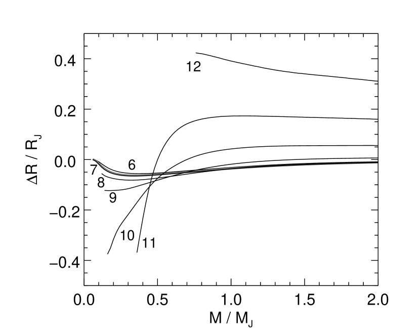
Figure 13: The ordinate is the radius difference $\Delta R=R_{\rm DFT-MD}-R_{\rm SC}$ for a given adiabat. The heavy shaded curve is for a Saturn adiabat with $S=$ 6.8. At low masses (below about 0.1 $M_{J}$ for low entropies) the difference goes to zero because there are no DFT-MD data at low densities.

The exoplanet HD 209458b (middle open data point in Figure 12) fortuitously falls near an entropy $S\approx 9.5$ $k_{b}$/el. and mass $M\approx 0.7M_{J}$ where $\Delta R\approx 0$. Nevertheless, the interior $T$-$\rho$ and $P$-$\rho$ profiles in figures 14 and 15 differ significantly between the DFT-MD and SC EOSs. These figures also compare interior profiles for simplified (pure H-He mixtures on an adiabat) models of Jupiter and Saturn.

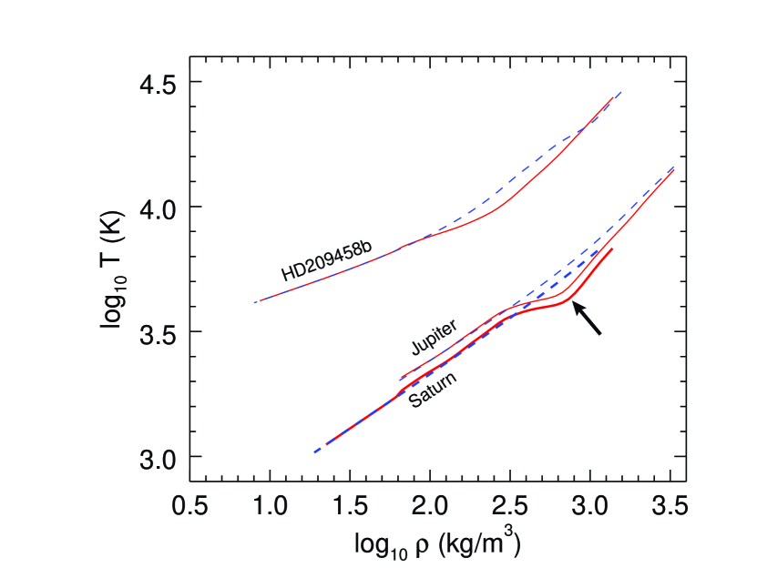
Figure 14: Temperature-density profile for the interior of three specific objects. Solid curves are for DFT-MD and dashed curves are for SC. The enhanced density in the DFT-MD model (see arrow) at pressures near $100$ GPa produces a slightly smaller radius for both Jupiter and Saturn. Below a density of 0.0670 g cm^-3, the SC model is used for both calculations.

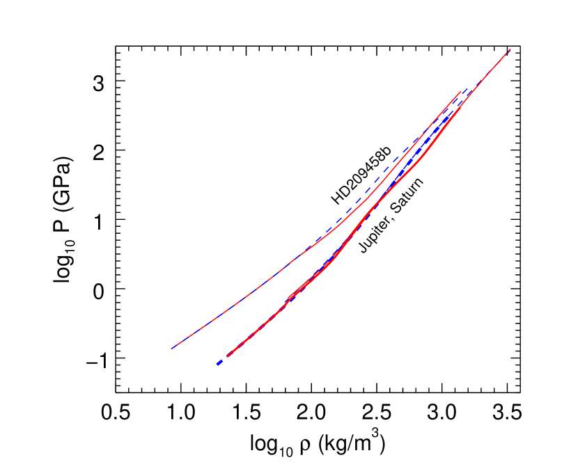
Figure 15: Pressure-density profile for the planetary interiors shown in Fig. 14.

Figure 16 shows differences in evolutionary behavior of our simplified planetary models. This figure plots the value of the central temperature, $T_{\rm central}$, vs. the central density, $\rho_{\rm central}$, for a range of adiabats and masses. During the evolution of a planet of constant mass, its central density increases monotonically while its central temperature exhibits a maximum. During the initial contraction, the temperature in the center increases at first as the material is subjected to increasing pressure. When a degenerate interior state is reached, the contraction ceases and the whole planet starts to cool. According to DFT-MD simulations the maximum temperature reached is up to 10 000 K lower than predicted by the SC model. This deviation may have consequences for the evolution of cores in giant planets that remain to be explored.

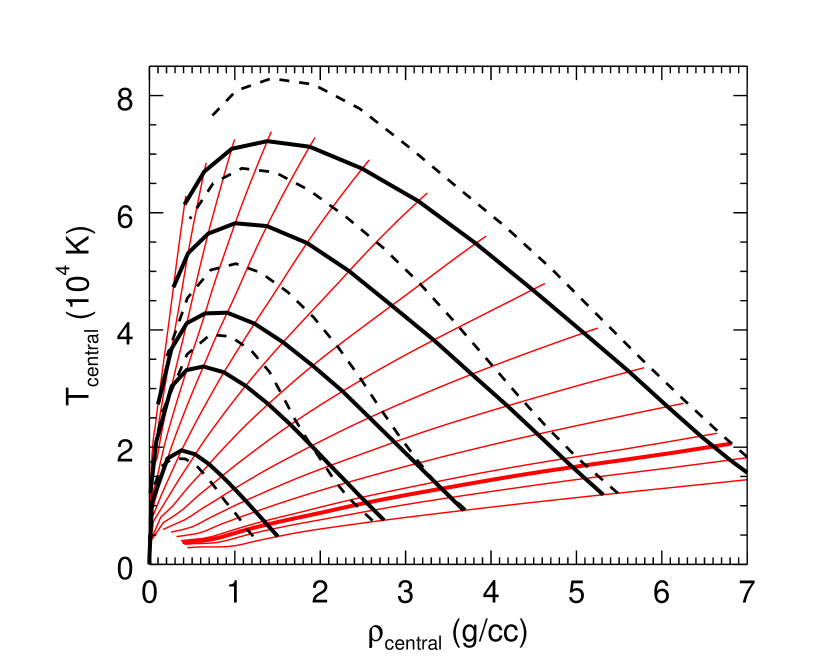
Figure 16: The values of $T$ and $\rho$ at the center of a planets according to the DFT-MD (heavy solid lines) and SC (dashed lines) EOSs for five different planet masses corresponding to 0.3 $M_{J}$ (Saturn, lowest curves), 0.7 $M_{J}$ (HD 209458b), 1.0 $M_{J}$ (Jupiter), 1.5 $M_{J}$, and 2.0 $M_{J}$ (top curves). The thin solid lines refer to various DFT-MD adiabats with entropy values from 6 (lowest curve) to 12 (steepest curve) in steps of 0.5 $k_{b}$/el. The heavy solid line is for Saturn’s entropy of 6.8.

7 Conclusions

This paper provides an equation state table for hydrogen-helium mixtures in giant planet interiors that was derived from ab initio computer simulations. The combination with an efficient thermodynamic integration technique enabled us to calculate the entropy and free energy directly, in addition to pressure and internal energy that follow from standard simulations.

Our complete EOS table with 391 density-temperature points as well as a thermodynamially consistent free energy fit is included in this publication so that our EOS can be easily incorporated in future models for giant planet interiors.

We have identified significant deviations for the Saumon and Chabrier EOS models. The new DFT-MD EOS causes low-entropy giant-planet models ($S\leq 8\,k_{b}$/el.) to shrink in comparison to SC models by up to 0.08 Jupiter radii. But for hot giant planets with mass exceeding $0.5\,M_{J}$ and with interior entropy values in the range from 10$-$12$\,k_{b}$/el., the DFT-MD simulations predict significantly larger radii. The correction to the SC model reaches 0.4 Jupiter radii for the hottest planets. Thus, the revision suggests that some of the most inflated giant exoplanets are at lower entropies than was previously inferred. Our revision could ameliorate the “inflated giant exoplanet” discrepancy to some extent but perhaps not for HD209458b. The matter is to be revisited with detailed evolutionary calculations based on our revised EOS.

Table 1: Equation of state derived from DFT-MD simulations.

$r_{s}$	Density	Temperature	Pressure	Internal Energy	Helmholtz Free	Entropy
($a_{0}$)	(g cm-3)	(K)	(GPa)	(Ha/el)	Energy (Ha/el)	($k_{b}$/el)
0.70	8.9658	5000	17713.9(3)	0.69251(3)	0.641237(7)	3.238(3)
0.80	6.0064	5000	8170.3(4)	0.41280(4)	0.351520(11)	3.870(3)
0.90	4.2185	5000	4064.5(3)	0.24343(4)	0.173088(24)	4.443(4)
1.00	3.0753	5000	2141.5(2)	0.13726(3)	0.058946(16)	4.946(3)
1.10	2.3105	5000	1180.6(2)	0.06926(6)	$-$0.016209(11)	5.398(4)
1.20	1.7797	5000	675.0(1)	0.02513(5)	$-$0.066864(21)	5.810(4)
1.30	1.3998	5000	398.4(1)	$-$0.00370(5)	$-$0.101600(16)	6.183(4)
1.40	1.1207	5000	242.1(1)	$-$0.02265(8)	$-$0.12587(3)	6.519(7)
1.50	0.9112	5000	151.8(2)	$-$0.03527(6)	$-$0.14310(4)	6.810(6)
1.60	0.7508	5000	98.0(1)	$-$0.04400(6)	$-$0.15565(2)	7.051(5)
1.86	0.4779	5000	38.2(1)	$-$0.05755(7)	$-$0.17565(3)	7.459(7)
2.00	0.3844	5000	25.74(8)	$-$0.06295(15)	$-$0.18271(4)	7.563(12)
2.10	0.3321	5000	19.97(9)	$-$0.06627(13)	$-$0.18655(4)	7.596(11)
2.20	0.2888	5000	15.51(9)	$-$0.0685(2)	$-$0.19015(4)	7.683(16)
2.30	0.2528	5000	12.24(7)	$-$0.0702(2)	$-$0.19312(5)	7.765(14)
2.40	0.2225	5000	9.64(6)	$-$0.0714(2)	$-$0.19580(7)	7.855(17)

Note. — Table 1 is published in its entirety in the electronic edition of the Astrophysical Journal. A portion is shown here for guidance regarding its form and content.

Table 2: Coefficients of Free Energy Fit for the equation of state.

	$r_{s}$	$T$	coefficient
	(a.u.)	(a.u.)	(a.u.)
$\frac{\partial F}{\partial T}$	1.75	0.001013	$-$8.67942$\times 10^{-1}$
$F$	1.75	0.001013	$-$9.23942$\times 10^{-2}$
$F$	1.75	0.003131	$-$9.76575$\times 10^{-2}$
$F$	1.75	0.006512	$-$1.12223$\times 10^{-1}$
$F$	1.75	0.011911	$-$1.44120$\times 10^{-1}$
$F$	1.75	0.020533	$-$2.07646$\times 10^{-1}$
$F$	1.75	0.034302	$-$3.23222$\times 10^{-1}$
$F$	1.75	0.056290	$-$5.29287$\times 10^{-1}$
$F$	1.75	0.091403	$-$8.92177$\times 10^{-1}$
$F$	1.75	0.147476	$-$1.53056
$F$	1.75	0.237021	$-$2.64345
$F$	1.75	0.380018	$-$4.58672
$\frac{\partial F}{\partial T}$	1.75	0.380018	$-$1.41575$\times 10^{+1}$

Note. — Table 2 is published in its entirety in the electronic edition of the Astrophysical Journal. A portion is shown here for guidance regarding its form and content. While this manuscript is still under review, a copy of the EOS fit as well as the computer interpolation program may be requested via email: militzer@berkeley.edu

References

- Alastuey & Ballenegger (2012) Alastuey, A. & Ballenegger, V. 2012, Phys. Rev. E, 86, 066402
- Batygin et al. (2011) Batygin, K., Stevenson, D. J., & Bodenheimer, P. 2011, ApJ, 738, 1
- Blöchl (1994) Blöchl, P. E. 1994, Phys. Rev. B, 50, 17953
- Bonev et al. (2004) Bonev, S. A., Militzer, B., & Galli, G. 2004, Phys. Rev. B, 69, 014101
- Burrows et al. (2007) Burrows, A., Hubeny, I., Budaj, J., & Hubbard, W. B. 2007, ApJ, 661, 502
- Caillabet et al. (2011) Caillabet, L., Mazevet, S., & Loubeyre, P. 2011, Phys. Rev. B, 83, 094101
- Chandrasekhar (1957) Chandrasekhar, S. 1957, Introduction to the Study of Stellar Structure (Dover), 84
- Collins et al. (2012) Collins, L. A., Kress, J. D., & Hanson, D. E. 2012, Phys. Rev. B, 85, 233101
- de Wijs et al. (1998) de Wijs, G. A., Kresse, G., & Gillan, M. J. 1998, Phys. Rev. B, 57, 8223
- Desjarlais (2003) Desjarlais, M. P. 2003, Phys. Rev. B, 68, 064204
- Dharma-wardana & Perrot (2002) Dharma-wardana, M. W. C. & Perrot, F. 2002, Phys. Rev. B, 66, 014110
- Driver & Militzer (2012) Driver, K. P. & Militzer, B. 2012, Phys. Rev. Lett., 108, 115502
- Ebeling et al. (2012) Ebeling, W., Kraeft, W., & Roepke, G. 2012, Contrib. Plasma Phys., 52, 7
- Fortney & Nettelmann (2010) Fortney, J. & Nettelmann, N. 2010, SSR, 152, 423
- Hamel et al. (2011) Hamel, S., Morales, M. A., & Schwegler, E. 2011, Phys. Rev. B, 84, 165110
- Hartman et al. (2011) Hartman, J. D., Bakos, G., Torres, G., Latham, D. W., Kovács, G., Béky, B., Quinn, S. N., Mazeh, T., Shporer, A., Marcy, G. W., Howard, A. W., Fischer, D. A., Johnson, J. A., Esquerdo, G. A., Noyes, R. W., Sasselov, D. D., Stefanik, R. P., Fernandez, J. M., Szklenár, T., Lázár, J., Papp, I., & Sári, P. 2011, ApJ, 742, 59
- Hu et al. (2010) Hu, S. X., Militzer, B., Goncharov, V. N., & Skupsky, S. 2010, Phys. Rev. Lett., 104, 235003
- Hu et al. (2011) —. 2011, Phys. Rev. B, 84, 224109
- Izvekov et al. (2003) Izvekov, S., Parrinello, M., Burnham, C. J., & Voth, G. A. 2003, J. Chem. Phys., 120, 10896
- Kohn & Sham (1965) Kohn, W. & Sham, L. 1965, Phys. Rev., 140, A1133
- Kraeft et al. (2002) Kraeft, W. D., Schlanges, M., Vorberger, J., & DeWitt, H. E. 2002, Phys. Rev. E, 66, 046405
- Kresse & Furthmüller (1996) Kresse, G. & Furthmüller, J. 1996, Phys. Rev. B, 54, 11169
- Laughlin et al. (2011) Laughlin, G., Crismani, M., & Adams, F. C. 2011, ApJ, 729, L7
- Lenosky et al. (2000) Lenosky, T. J., Bickham, S. R., Kress, J. D., & Collins, L. A. 2000, Phys. Rev. B, 61, 1
- Magro et al. (1996) Magro, W. R., Ceperley, D. M., Pierleoni, C., & Bernu, B. 1996, Phys. Rev. Lett., 76, 1240
- McMahon et al. (2012) McMahon, J. M., Morales, M. A., Pierleoni, C., & Ceperley, D. M. 2012, Rev. Mod. Phys., 84, 1607
- Mermin (1965) Mermin, N. D. 1965, Phys. Rev., 137, A1441
- Militzer (2005) Militzer, B. 2005, J. Low Temp. Phys., 139, 739
- Militzer (2006) —. 2006, Phys. Rev. Lett., 97, 175501
- Militzer (2009) —. 2009, Phys. Rev. B, 79, 155105
- Militzer (2013) —. 2013, Phys. Rev. B, 87, 014202
- Militzer & Ceperley (2000) Militzer, B. & Ceperley, D. M. 2000, Phys. Rev. Lett., 85, 1890
- Militzer & Ceperley (2001) —. 2001, Phys. Rev. E, 63, 066404
- Militzer et al. (2001) Militzer, B., Ceperley, D. M., Kress, J. D., Johnson, J. D., Collins, L. A., & Mazevet, S. 2001, Phys. Rev. Lett., 87, 275502
- Militzer & Graham (2006) Militzer, B. & Graham, R. L. 2006, Journal of Physics and Chemistry of Solids, 67, 2136
- Militzer & Hubbard (2009) Militzer, B. & Hubbard, W. H. 2009, Astrophys. and Space Sci., 322, 129
- Militzer et al. (2008) Militzer, B., Hubbard, W. H., Vorberger, J., Tamblyn, I., & Bonev, S. A. 2008, Astrophys. J. Lett., 688, L45
- Militzer et al. (1999) Militzer, B., Magro, W., & Ceperley, D. 1999, Contr. Plasma Physics, 39 1-2, 152
- Miller & Fortney (2011) Miller, N. & Fortney, J. 2011, ApJ, 736, L29
- Morales et al. (2009) Morales, M. A., Pierleoni, C., Schwegler, E., & Ceperley, D. M. 2009, Proc. Nat. Acad. Sci., 106, 1324
- Morales et al. (2010) —. 2010, Proc. Nat. Acad. Sci., 107, 12799
- Nettelmann et al. (2012) Nettelmann, N., Becker, A., Holst, B., & Redmer, R. 2012, Astrophys. J., 750, 52
- Nettelmann et al. (2008) Nettelmann, N., Holst, B., Kietzmann, A., French, M., Redmer, R., & Blaschke, D. 2008, Astrophys. J., 683, 1217
- Perdew et al. (1996) Perdew, J. P., Burke, K., & Ernzerhof, M. 1996, Phys. Rev. Lett., 77, 3865
- Pierleoni et al. (1994) Pierleoni, C., Ceperley, D., Bernu, B., & Magro, W. 1994, Phys. Rev. Lett., 73, 2145
- Rogers & Nayfonov (2002) Rogers, J. & Nayfonov, A. 2002, Astrophys. J., 576, 1064
- Safa & Pfenniger (2008) Safa, Y. & Pfenniger, D. 2008, Eur. Phys. J. B, 66, 337
- Saumon & Chabrier (1992) Saumon, D. & Chabrier, G. 1992, Phys. Rev. A, 46, 2084
- Saumon et al. (1995) Saumon, D., Chabrier, G., & Horn, H. M. V. 1995, Astrophys. J. Suppl., 99, 713
- Schneider et al. (2011) Schneider, J., Dedieu, C., Sidaner, P. L., Savalle, R., & Zolotukhin, I. 2011, AAp, 532, A79
- Stevenson & Salpeter (1977) Stevenson, D. & Salpeter, E. 1977, Astrophys. J. Suppl. Ser., 35, 221
- Stixrude & Jeanloz (2008) Stixrude, L. & Jeanloz, R. 2008, Proc. Nat. Ac. Sci., 105, 11071
- Vorberger et al. (2007a) Vorberger, J., Tamblyn, I., Bonev, S., & Militzer, B. 2007a, Contrib. Plasma Phys., 47, 375
- Vorberger et al. (2007b) Vorberger, J., Tamblyn, I., Militzer, B., & Bonev, S. 2007b, Phys. Rev. B, 75, 024206
- Wilson & Militzer (2010) Wilson, H. F. & Militzer, B. 2010, Phys. Rev. Lett., 104, 121101
- Wilson & Militzer (2012a) —. 2012a, Astrophys. J, 745, 54
- Wilson & Militzer (2012b) —. 2012b, Phys. Rev. Lett., 108, 111101