Regularity criteria of weak solutions to NSE in some bounded domains involving the pressure

Abstract.

We present a short and elegant proof of the inequality $\left\lVert p\right\rVert_{L_{s}(\Omega)}\leq c(\Omega)\left(\left\lVert v\right\rVert^{2}_{L_{2s}(\Omega)}+\left\lVert f\right\rVert_{L_{s}(\Omega)}\right)$ for bounded domains $\Omega$ under the slip and Navier boundary conditions. We also show an application of this result for conditional regularity of weak solutions to the Navier-Stokes equations.

1. Introduction

We consider the initial-boundary value problem for the Navier-Stokes equations

(1.1) $$v_{,t}+(v\cdot\nabla)v-\nu\triangle v+\nabla p=f \text{in $\Omega\times(0,T)=:\Omega^{T}$},$$

$$\operatorname{div}v=0 \text{in $\Omega^{T}$},$$

$$v|_{t=0}=v(0) \text{in $\Omega$},$$

either with boundary slip conditions

(1.2) $$\begin{aligned} &n\cdot\mathbb{D}(v)\cdot\tau^{\alpha}=0,\\ &n\cdot v=0\end{aligned} \partial\Omega$$ on

or with the Navier boundary conditions

(1.3) $$\begin{aligned} &\operatorname{rot}v\times n=0,\\ &n\cdot v=0\end{aligned} \partial\Omega$$ on ,

where $\Omega\subset\mathbb{R}^{3}$ is a bounded domain. In case of the boundary slip conditions it is more convenient to write (1.1)₁ in the form

(1.4) $$v_{,t}+(v\cdot\nabla)v-\operatorname{div}\mathbb{T}(v,p)=f.$$

To make the above conditions clear let us recall that $n$ and $\tau^{\alpha}$, $\alpha\in\{1,2\}$ are the unit outward normal vector and the unit tangent vectors. By $\mathbb{T}(v,p)$ we mean the stress tensor

$$\mathbb{T}(v,p)=\nu\mathbb{D}(v)-p\mathbb{I},$$

where $\mathbb{D}(v)$ is the dilatation tensor, which equals $\frac{1}{2}\left(\nabla v+\nabla^{\perp}v\right)$, $\mathbb{I}$ is the unit matrix and $\nu>0$ represents the viscosity coefficient.

Note that (1.3) is sometimes referred also as a boundary slip condition whereas (1.2) as the Navier boundary condition. In some cases these conditions coincide (i.e. $\Omega$ is half-space) but in general they differ. In certain cases this difference can be measured in term of the curvature of $\partial\Omega$ (for $\Omega$ of cylindrical type see e.g. [Now13, Lemma 6.5]) but this issue is beyond the scope of our work.

It is well known that for $v(0)\in H^{1}(\Omega)$ there exists at least one weak solution (see e.g. [Hop50], [Gal00]), but the problem of uniqueness and regularity of weak solution in three dimensions remains open.

Our primary interest in (1.1) is an extension of the regularity criterion for the weak solutions onto bounded domains under boundary slip type conditions. One of the basic ideas used in the proof would rely on testing (1.1) with $v\left\lvert v\right\rvert^{\theta-2}$, $\theta\geq 2$. This approach leads to a difficulty related to the estimate for the pressure term. In the whole space or in periodic setting it can be resolved by the application of the Calderón-Zygmund theorem (see e.g. [Str07]) to the equation

(1.5) $$-\triangle p=\sum_{i,j=1}^{3}\frac{\partial^{2}}{\partial x_{i}\partial x_{j}}\left(v_{i}v_{j}\right),$$

thereby yielding the following estimate

(1.6) $$\left\lVert p\right\rVert_{L_{s}(\Omega)}\leq\left\lVert v\right\rVert_{L_{2s}(\Omega)}^{2}.$$

Clearly, in bounded domains (1.5) must be supplemented with some boundary condition, which at large are difficult or even impossible to establish due to lack of information on $p$ or $\frac{\partial p}{\partial n}$ on $\partial\Omega$ in terms of $v$. One of effective, but restrictive to particular cases remedies that may be exhausted lies in e.g. choosing axially symmetric cylinders with boundary slip conditions (see e.g. [Zaj04, Ch. 3, Lemma 1.1]). One can put another restrictions on the geometry of the domain or on the boundary conditions but at the end we lose certain generality. Therefore, it is reasonable to look for any estimates to for the pressure without the necessity of analyzing (1.5).

In this paper we give an alternative proof of the estimate of the form of (1.6), which indeed does not rely on (1.5). In principle, it is based on an auxiliary Poisson equation with the Neumann boundary conditions. The result reads:

Theorem 1.

Suppose that $f\in L_{s}(\Omega)$ and $v\in L_{2s}(\Omega)$ satisfy (1.1). Let (1.3) hold and $\Omega$ is bounded and sufficiently regular. Then $p\in L_{s}(\Omega)$ and

$$\left\lVert p\right\rVert_{L_{s}(\Omega)}\leq c(\Omega)\left(\left\lVert v\right\rVert_{L_{2s}(\Omega)}^{2}+\left\lVert f\right\rVert_{L_{s}(\Omega)}\right).$$

Let now (1.2) hold. If in addition $\nabla v\in L_{s}(\Omega)$, then

$$\left\lVert p\right\rVert_{L_{s}(\Omega)}\leq c(\Omega)\left(\left\lVert v\right\rVert_{L_{2s}(\Omega)}^{2}+\left\lVert\nabla v\right\rVert_{L_{s}(\Omega)}+\left\lVert f\right\rVert_{L_{s}(\Omega)}\right).$$

Remark 1.1.

The regularity requirement concerning the domain $\Omega$ is related to the Neumann problem for the Poisson equation. For a given $s$ the set $\Omega$ is sufficiently regular if for each $g\in L_{s^{\prime}}(\Omega)$ such that $\int_{\Omega}g\,\mathrm{d}x=0$ the following problem

(1.7) $$-\triangle\psi=g\, \text{in $\Omega$},$$

$$n\cdot\nabla\psi=0 \text{on $S$},$$

$$\int_{\Omega}\psi=0,$$

has the unique solution $u\in W^{2}_{s^{\prime}}(\Omega)$, where $\frac{1}{s}+\frac{1}{s^{\prime}}=1$. It holds, for example, if:

• $\partial\Omega\in C^{1,1}$, $s>1$ (see [Gri85, Lemma 2.4.2.1])

• $\Omega$ is convex, $s\in[2,\infty)$ (see [AJ94]),

• $\Omega\subset\mathbb{R}^{3}$ is a bounded, convex polyhedron and

  $$1<\frac{s}{s-1}<\min\left\{3,\frac{2\alpha_{E}}{(2\alpha_{E}-\pi)_{+}}\right\},$$

  where $\alpha_{E}$ is opening of the dihedral angle with edge $E$ (see [Maz09]),

• $\Omega=[0,a]\times[0,b]\times[0,c]$, $s>1$ (the reflection argument),

• $\Omega=[0,a]\times\Omega^{\prime}$, where $\Omega^{\prime}\subset\mathbb{R}^{2}$ is a bounded set with a smooth boundary, $s>1$ (the reflection argument).

Clearly, apart the already mentioned idea, there are different techniques that could be utilized to analyze problem (1.1) with or without relying on (1.5). It was a great surprise that they seem to work only in case of the Dirichlet boundary conditions (see [Cho98], [BG02, Sec. 3], [Zho04], [KL06], [FKS09], [Kim10]), whereas the boundary slip type conditions were only considered in the half space (see [BJ08] and [BCJ08]) or in the case of axially symmetric solutions (see [Zaj10]). In our work we achieve a little progress. Although the domain we work with is bounded but we assume that it is of cubical type. This kind of restriction, tightly related to the boundary integrals, is removable in many cases (see Remark 4.2). Our major motivation for investigating the simplest domain follows from intention of keeping the calculations clear and simple. The result reads:

Theorem 2.

Let $f\equiv 0$, $T>0$ and $\Omega:=[0,a]\times[0,b]\times[0,c]$ for finite, positive real constants $a$, $b$ and $c$. Suppose that a weak solution $v$ to (1.1) supplemented with either (1.2) or (1.3) satisfies

$$\left\lVert v\right\rVert_{L_{q}(0,T;L_{p}(\Omega))}<+\infty\qquad\text{where}\qquad\frac{3}{p}+\frac{2}{q}=1$$

for $q<+\infty$. Then, $v$ is unique and smooth.

Remark 1.2.

The assumption $f\equiv 0$ is artificial and can be omitted. It does not change the proof but makes it a little longer.

Remark 1.3.

For the definition and the proof of existence of weak solutions to (1.1) supplemented with (1.2) or (1.3) see e.g. Introduction in [Zaj05b].

Remark 1.4.

If we drop the assumption on the cubical shape of the domain, the claim of Theorem 2 in case $q<+\infty$ is still true. The proof is different, easier but does not base on Theorem 1. We will present its sketch at the end of this work.

Remark 1.5.

In cubical domains under both boundary conditions (1.2) and (1.3) the assertion of Theorem 1 reads

$$\left\lVert p\right\rVert_{L_{s}(\Omega)}\leq c(\Omega)\left(\left\lVert v\right\rVert_{L_{2s}(\Omega)}^{2}+\left\lVert f\right\rVert_{L_{s}(\Omega)}\right).$$

Before we move to the next section, let us note that the extension of Serrin condition is mostly studied for the Cauchy problem (see e.g. [KS04], [KZ06], [Zho06], [CT08], [BV11], [PP11]) or for the local-interior regularity (see e.g. [GKT06]), thereby excluding the boundary issues. We do not intend to compare or discuss these improvements. This has been nicely done in several papers. The interested reader we would refer e.g. to [Ber09].

2. Auxiliary results

Throughout this article we use the following Young inequality:

Lemma 2.1 (The Young inequality with small parameter $\kappa$).

For any positive $a$ and $b$ the inequality

$$ab\leq\kappa a^{\lambda_{1}}+(\kappa\lambda_{1})^{-\frac{\lambda_{2}}{\lambda_{1}}}\lambda_{2}^{-1}b^{\lambda_{2}}$$

holds, where $\kappa>0$ and

$$\frac{1}{\lambda_{1}}+\frac{1}{\lambda_{2}}=1,\qquad 1<\lambda_{1},\lambda_{2}<+\infty.$$

Another useful tool is the imbedding lemma for the space $V^{k}_{2}(\Omega^{t})$, which is defined as the closure of $\mathcal{C}^{\infty}(\Omega\times(t_{0},t_{1}))$ in the norm

$$\left\lVert u\right\rVert_{V^{k}_{2}(\Omega^{t})}^{2}=\underset{t\in(t_{0},t_{1})}{\operatorname{ess\,sup}}\left\lVert u(t)\right\rVert_{H^{k}(\Omega)}^{2}\\ +\left(\int_{t_{0}}^{t_{1}}\left\lVert\nabla u(t)\right\rVert^{2}_{H^{k}(\Omega)}\,\mathrm{d}t\right)^{1/2}.$$

The imbedding lemma reads:

Lemma 2.2.

Suppose that $u\in V_{2}^{0}(\Omega^{t})$, where $\Omega^{t}:=\Omega\times(t_{0},t)$, $t_{0}<t\leq t_{1}$. Then $u\in L_{q}(t_{0},t;L_{p}(\Omega))$ and

$$\left\lVert u\right\rVert_{L_{q}(t_{0},t;L_{p}(\Omega))}\leq c(p,q,\Omega)\left\lVert u\right\rVert_{V^{0}_{2}(\Omega^{t})}$$

holds under the condition $\frac{3}{p}+\frac{2}{q}=\frac{3}{2}$, $2\leq p\leq 6$.

Let us emphasize that the constant that appears on the right-hand side does not depend on time.

Lemma 2.3 (Imbedding theorem).

Let $\Omega$ satisfy the cone condition and let $q\geq p$. Set

$$\kappa=2-2r-s-5\left(\frac{1}{p}-\frac{1}{q}\right)\geq 0.$$

Then for any function $u\in W^{2,1}_{p}(\Omega^{t})$ the inequality

$$\left\lVert\partial^{r}_{t}\mathrm{D}_{x}^{s}u\right\rVert_{L_{q}(\Omega^{t})}\leq c_{1}(p,q,r,s,\Omega)\epsilon^{\kappa}\left\lVert u\right\rVert_{W^{2,1}_{p}(\Omega^{t})}+c_{2}(p,q,r,s,\Omega)\epsilon^{-\kappa+2s-2}\left\lVert u\right\rVert_{L_{p}(\Omega^{t})}$$

holds, where the constants $c_{1}$ and $c_{2}$ do not depend on $t$.

For the proof of the lemma we refer the reader to [LSU67, Ch.2, §3, Lemma 3.3].

3. Proof of Theorem 1

Proof.

Let $\psi\in W^{2}_{s^{\prime}}(\Omega)$ be a unique solution to the following elliptic problem:

(3.1) $$-\triangle\psi=p\left\lvert p\right\rvert^{s-2}-\frac{1}{\left\lvert\Omega\right\rvert}\int_{\Omega}p\left\lvert p\right\rvert^{s-2}\,\mathrm{d}x \text{in $\Omega$},$$

$$n\cdot\nabla\psi=0 \text{on $S$},$$

$$\int_{\Omega}\psi\,\mathrm{d}x=0.$$

Then the estimate

(3.2) $$\left\lVert\psi\right\rVert_{W^{2}_{s^{\prime}}(\Omega)}\leq c(s,\Omega)\left\lVert p\right\rVert^{s-1}_{L_{s}(\Omega)}$$

holds. Multiplying (1.1)₁ by $\nabla\psi$ and integrating over $\Omega$ yields

(3.3) $$\int_{\Omega}\big{(}v_{,t}-\nu\triangle v+v\cdot\nabla v+\nabla p\big{)}\cdot\nabla\psi\,\mathrm{d}x=\int_{\Omega}f\cdot\nabla\psi\,\mathrm{d}x.$$

We have four integral on the left-hand side which need to be estimated. First we see

(3.4) $$\int_{\Omega}v_{,t}\cdot\nabla\psi\,\mathrm{d}x=\int_{\Omega}\big{(}\nabla\cdot(v_{,t}\psi)-\operatorname{div}v_{,t}\psi\big{)}\,\mathrm{d}x=\int_{S}\psi(v_{,t}\cdot n)\,\mathrm{d}S=0.$$

The estimate for the second integral varies in dependence on the boundary conditions. Let us assume (1.3) first. Condition (1.2) will be discussed at the end of the proof. Thus,

$$\int_{\Omega}\triangle v\cdot\nabla\psi\,\mathrm{d}x=-\int_{\Omega}\operatorname{rot}\operatorname{rot}v\cdot\nabla\psi\,\mathrm{d}x=-\int_{S}\operatorname{rot}v\times n\cdot\nabla\psi\,\mathrm{d}S=0.$$

For the third integral we have

$$\int_{\Omega}v_{i}v_{j,x_{i}}\psi_{,x_{j}}\,\mathrm{d}x=-\int_{\Omega}v_{i}v_{j}\psi_{,x_{j}x_{i}}\,\mathrm{d}x+\int_{S}v_{i}v_{j}\psi_{,x_{j}}n_{i}\,\mathrm{d}S\leq\left\lVert v\right\rVert^{2}_{L_{2s}(\Omega)}\left\lVert\nabla^{2}\psi\right\rVert_{L_{s^{\prime}}(\Omega)},$$

where we integrated by parts and utilized equality (1.3)₂. The last term on the left-hand side in (3.3) is equal to

(3.5) $$-\int_{\Omega}p\cdot\triangle\psi\,\mathrm{d}x+\int_{S}p\left(n\cdot\nabla\psi\right)\,\mathrm{d}S=-\int_{\Omega}\left\lvert p\right\rvert^{s}\mathrm{d}x+\frac{1}{\left\lvert\Omega\right\rvert}\left(\int_{\Omega}p\left\lvert p\right\rvert^{s-2}\,\mathrm{d}x\right)\,\int_{\Omega}p\,\mathrm{d}x=-\left\lVert p\right\rVert_{L_{s}(\Omega)}^{s},$$

because the boundary integral is equal to zero due to (3.1)₂ and $p$ is a distribution determined up to a constant.

Finally, by the Hölder inequality

$$\int_{\Omega}f\cdot\nabla\psi\,\mathrm{d}x\leq\left\lVert f\right\rVert_{L_{s}(\Omega)}\left\lVert\nabla\psi\right\rVert_{L_{s^{\prime}}(\Omega)}.$$

Summing up the above estimates and in view of (3.2) we obtain

$$\left\lVert p\right\rVert_{L_{s}(\Omega)}^{s}\leq\left\lVert v\right\rVert^{2}_{L_{2s}(\Omega)}\left\lVert\nabla^{2}\psi\right\rVert_{L_{s^{\prime}}(\Omega)}+\left\lVert f\right\rVert_{L_{s}(\Omega)}\left\lVert\nabla\psi\right\rVert_{L_{s^{\prime}}(\Omega)}\leq c(\Omega)\left\lVert p\right\rVert^{s-1}_{L_{s}(\Omega)}\left(\left\lVert v\right\rVert_{L_{2s}(\Omega)}^{2}+\left\lVert f\right\rVert_{L_{s}(\Omega)}\right).$$

Hence

$$\left\lVert p\right\rVert_{L_{s}(\Omega)}\leq c(\Omega)\left(\left\lVert v\right\rVert_{L_{2s}(\Omega)}^{2}+\left\lVert f\right\rVert_{L_{s}(\Omega)}\right),$$

which concludes the proof of the first assertion.

Let now (1.2) hold. Then, instead of (3.3) we have in light of (1.4) the identity

(3.6) $$\int_{\Omega}\big{(}v_{,t}-\operatorname{div}\mathbb{T}(v,p)+v\cdot\nabla v\big{)}\cdot\nabla\psi\,\mathrm{d}x=\int_{\Omega}f\cdot\nabla\psi\,\mathrm{d}x.$$

We need to examine the term involving the Cauchy stress tensor. We see that

(3.7) $$\int_{\Omega}-\operatorname{div}\mathbb{T}(v,p)\cdot\nabla\psi\,\mathrm{d}x\\ =-\int_{S}n\cdot\nu\mathbb{D}(v)\cdot\nabla\psi\,\mathrm{d}S+\int_{S}p\left(\nabla\psi\cdot n\right)\,\mathrm{d}S+\int_{\Omega}\nu\mathbb{D}(v)\nabla^{2}\psi\,\mathrm{d}x+\int_{\Omega}p\triangle\psi\,\mathrm{d}x.$$

Expressing $\mathbb{D}(v)$ in the basis $n,\tau^{\alpha}$, $\alpha=1,2$ yields

$$\int_{S}n\cdot\nu\mathbb{D}(v)\cdot\nabla\psi\,\mathrm{d}S=\nu\int_{S}\left(n\cdot\mathbb{D}(v)\cdot n\right)n\cdot\nabla\psi\,\mathrm{d}S+\nu\int_{S}\left(n\cdot\mathbb{D}(v)\cdot\tau^{\alpha}\right)\tau^{\alpha}\cdot\nabla\psi\,\mathrm{d}S.$$

The first integral vanishes due to (3.1)₂, whereas the second due to (1.2). Combining (3.4), (3.5) and (3.7) we infer from (3.6) that

$$\left\lVert p\right\rVert_{L_{s}(\Omega)}^{s}\leq\left\lVert v\right\rVert^{2}_{L_{2s}(\Omega)}\left\lVert\nabla^{2}\psi\right\rVert_{L_{s^{\prime}}(\Omega)}+\left\lVert\nabla v\right\rVert_{L_{s}(\Omega)}\left\lVert\nabla^{2}\psi\right\rVert_{L_{s^{\prime}}(\Omega)}+\left\lVert f\right\rVert_{L_{s}(\Omega)}\left\lVert\nabla\psi\right\rVert_{L_{s^{\prime}}(\Omega)}\\ \leq c(\Omega)\left\lVert p\right\rVert^{s-1}_{L_{s}(\Omega)}\left(\left\lVert v\right\rVert_{L_{2s}(\Omega)}^{2}+\left\lVert\nabla v\right\rVert_{L_{s}(\Omega)}+\left\lVert f\right\rVert_{L_{s}(\Omega)}\right),$$

which is our second assertion. The proof is complete. ∎

4. Proof of Theorem 2

Proof.

We start with multiplying (1.1) by $v\left\lvert v\right\rvert^{\theta-2}$ and integrating over $\Omega$

(4.1) $$\frac{1}{\theta}\operatorname{\frac{\mathrm{d}}{\mathrm{d}t}}\int_{\Omega}\left\lvert v\right\rvert^{\theta}\,\mathrm{d}x+\nu\int_{\Omega}\nabla v\cdot\nabla\left(v\left\lvert v\right\rvert^{\theta-2}\right)\,\mathrm{d}x=-\int_{\Omega}\nabla p\cdot v\left\lvert v\right\rvert^{\theta-2}\,\mathrm{d}x+\int_{S}\sum_{i,j=1}^{3}v_{j,x_{i}}\cdot v_{j}\left\lvert v\right\rvert^{\theta-2}\cdot n_{i}\,\mathrm{d}S,$$

where $\theta>3$ and the non-linear term vanishes due to

$$\int_{\Omega}(v\cdot\nabla)v\cdot v\left\lvert v\right\rvert^{\theta-2}\,\mathrm{d}x=\frac{1}{2}\int_{\Omega}v_{i}\left(v\cdot v\right)_{,x_{i}}\left\lvert v\right\rvert^{\theta-2}\,\mathrm{d}x=\frac{1}{\theta}\int_{\Omega}v_{i}\left(\left\lvert v\right\rvert^{2}\right)^{\frac{\theta}{2}}_{,x_{i}}\,\mathrm{d}x\\ =-\frac{1}{\theta}\int_{\Omega}\operatorname{div}v\left\lvert v\right\rvert^{\theta}\,\mathrm{d}x+\frac{1}{\theta}\int_{S}\left\lvert v\right\rvert^{\theta}\left(v\cdot n\right)\,\mathrm{d}S=0.$$

Consider first the boundary integral on the right-hand side. On the walls $x_{3}=0$ and $x_{3}=c$ the normal vector $n$ equals $(0,0,\mp 1)$ and conditions (1.2), (1.3) imply $v_{1,x_{3}}=v_{2,x_{3}}=v_{3}=0$ (see [Zaj05b, Lemma 3.1 and its proof] and [Now13, Lemma 6.6], respectively). Therefore

$$\int_{S\cap x_{3}\in\{0,c\}}\sum_{i,j=1}^{3}v_{j,x_{i}}\cdot v_{j}\left\lvert v\right\rvert^{\theta-2}\cdot n_{i}\,\mathrm{d}S=0.$$

Following nearly identical reasoning for $x_{2}\in\{0,b\}$ and $x_{1}\in\{0,a\}$ we conclude that

$$\int_{S}\sum_{i,j=1}^{3}v_{j,x_{i}}\cdot v_{j}\left\lvert v\right\rvert^{\theta-2}\cdot n_{i}\,\mathrm{d}S=0.$$

For the second term on the left-hand side in (4.1) we have

$$\nu\int_{\Omega}\nabla v\cdot\nabla\left(v\left\lvert v\right\rvert^{\theta-2}\right)\,\mathrm{d}x=\nu\int_{\Omega}\left\lvert\nabla v\right\rvert^{2}\left\lvert v\right\rvert^{\theta-2}\,\mathrm{d}x+\frac{4\nu(\theta-2)}{\theta^{2}}\int_{\Omega}\left\lvert\nabla\left\lvert v\right\rvert^{\frac{\theta}{2}}\right\rvert^{2}\,\mathrm{d}x.$$

To estimate the term with the pressure we integrate by parts and use (1.1)₂ and boundary conditions

$$-\int_{\Omega}\nabla p\cdot v\left\lvert v\right\rvert^{\theta-2}\,\mathrm{d}x=\left(\frac{\theta}{2}-1\right)\int_{\Omega}p|v|^{\theta-4}v\cdot\nabla\left\lvert v\right\rvert^{2}\,\mathrm{d}x\leq(\theta-2)\int_{\Omega}\left\lvert p\right\rvert\left\lvert v\right\rvert^{\frac{\theta}{2}-1}\left\lvert\nabla v\right\rvert\left\lvert v\right\rvert^{\frac{\theta}{2}-1}\,\mathrm{d}x.$$

From the Cauchy inequality we immediately get

$$(\theta-2)\int_{\Omega}\left\lvert p\right\rvert\left\lvert v\right\rvert^{\frac{\theta}{2}-1}\left\lvert\nabla v\right\rvert\left\lvert v\right\rvert^{\frac{\theta}{2}-1}\,\mathrm{d}x\leq(\theta-2)\left(\int_{\Omega}\left\lvert p\right\rvert^{2}\left\lvert v\right\rvert^{\theta-2}\,\mathrm{d}x\right)^{\frac{1}{2}}\left(\int_{\Omega}\left\lvert\nabla v\right\rvert^{2}\left\lvert v\right\rvert^{\theta-2}\,\mathrm{d}x\right)^{\frac{1}{2}}.$$

So far we have obtained

(4.2) $$\frac{1}{\theta}\operatorname{\frac{\mathrm{d}}{\mathrm{d}t}}\int_{\Omega}\left\lvert v\right\rvert^{\theta}\,\mathrm{d}x+\frac{4\nu(\theta-2)}{\theta^{2}}\int_{\Omega}\left\lvert\nabla\left\lvert v\right\rvert^{\frac{\theta}{2}}\right\rvert^{2}\,\mathrm{d}x+\nu\int_{\Omega}\left\lvert\nabla v\right\rvert^{2}\left\lvert v\right\rvert^{\theta-2}\,\mathrm{d}x\\ \leq(\theta-2)\left(\int_{\Omega}\left\lvert p\right\rvert^{2}\left\lvert v\right\rvert^{\theta-2}\,\mathrm{d}x\right)^{\frac{1}{2}}\left(\int_{\Omega}\left\lvert\nabla v\right\rvert^{2}\left\lvert v\right\rvert^{\theta-2}\,\mathrm{d}x\right)^{\frac{1}{2}}.$$

To estimate the right-hand side we use the Hölder inequality

$$\left(\int_{\Omega}\left\lvert p\right\rvert^{2}\left\lvert v\right\rvert^{\theta-2}\,\mathrm{d}x\right)^{\frac{1}{2}}\left(\int_{\Omega}\left\lvert\nabla v\right\rvert^{2}\left\lvert v\right\rvert^{\theta-2}\,\mathrm{d}x\right)^{\frac{1}{2}}\\ \leq\left(\left(\int_{\Omega}\left\lvert p\right\rvert^{2\lambda_{1}}\,\mathrm{d}x\right)^{\frac{1}{\lambda_{1}}}\left(\int_{\Omega}\left\lvert v\right\rvert^{(\theta-2)\lambda_{2}}\,\mathrm{d}x\right)^{\frac{1}{\lambda_{2}}}\right)^{\frac{1}{2}}\left(\int_{\Omega}\left\lvert\nabla v\right\rvert^{2}\left\lvert v\right\rvert^{\theta-2}\,\mathrm{d}x\right)^{\frac{1}{2}}.$$

By Remark 1.5

$$\left(\int_{\Omega}\left\lvert p\right\rvert^{2\lambda_{1}}\,\mathrm{d}x\right)^{\frac{1}{2\lambda_{1}}}\leq c(\Omega)\left(\int_{\Omega}\left\lvert v\right\rvert^{4\lambda_{1}}\,\mathrm{d}x\right)^{\frac{2}{4\lambda_{1}}}=c(\Omega)\left\lVert v\right\rVert_{L_{4\lambda_{1}}(\Omega)}^{2},$$

which combined with (4.2) yields

(4.3) $$\frac{1}{\theta}\operatorname{\frac{\mathrm{d}}{\mathrm{d}t}}\int_{\Omega}\left\lvert v\right\rvert^{\theta}\,\mathrm{d}x+\frac{4\nu(\theta-2)}{\theta^{2}}\int_{\Omega}\left\lvert\nabla\left\lvert v\right\rvert^{\frac{\theta}{2}}\right\rvert^{2}\,\mathrm{d}x+\nu\int_{\Omega}\left\lvert\nabla v\right\rvert^{2}\left\lvert v\right\rvert^{\theta-2}\,\mathrm{d}x\\ \leq c(\Omega)(\theta-2)\left\lVert v\right\rVert_{L_{4\lambda_{1}}(\Omega)}^{2}\left\lVert v\right\rVert_{L_{(\theta-2)\lambda_{2}}(\Omega)}^{\frac{\theta-2}{2}}\left(\int_{\Omega}\left\lvert\nabla v\right\rvert^{2}\left\lvert v\right\rvert^{\theta-2}\,\mathrm{d}x\right)^{\frac{1}{2}}.$$

Due to the imbedding $H^{1}(\Omega)\hookrightarrow L_{6}(\Omega)$ and the Poincaré inequality (every component of $v$ vanishes on different part of the boundary) we see that

(4.4) $$\int_{\Omega}\left\lvert\nabla\left\lvert v\right\rvert^{\frac{\theta}{2}}\right\rvert^{2}\,\mathrm{d}x\geq c(\Omega)\left(\int_{\Omega}\left\lvert v\right\rvert^{\frac{\theta}{2}\cdot 6}\,\mathrm{d}x\right)^{\frac{1}{6}\cdot 2}=c(\Omega)\left\lVert v\right\rVert_{L_{3\theta}(\Omega)}^{\theta}.$$

Therefore we interpolate $L_{4\lambda_{1}}(\Omega)$ and $L_{(\theta-2)\lambda_{2}}(\Omega)$ between $L_{\theta}(\Omega)$ and $L_{3\theta}(\Omega)$:

$$\frac{1}{4\lambda_{1}} =\frac{\alpha}{\theta}+\frac{1-\alpha}{3\theta}=\frac{2\alpha+1}{3\theta} \Leftrightarrow \alpha=\frac{1}{2}\left(\frac{3\theta}{4\lambda_{1}}-1\right)=\frac{3\theta-4\lambda_{1}}{8\lambda_{1}},$$

$$\frac{1}{(\theta-2)\lambda_{2}} =\frac{\beta}{\theta}+\frac{1-\beta}{3\theta}=\frac{2\beta+1}{3\theta} \Leftrightarrow \beta=\frac{1}{2}\left(\frac{3\theta}{(\theta-2)\lambda_{2}}-1\right)=\frac{3\theta-(\theta-2)\lambda_{2}}{2(\theta-2)\lambda_{2}}$$

and

$$1-\alpha =1-\frac{3\theta-4\lambda_{1}}{8\lambda_{1}}=\frac{12\lambda_{1}-3\theta}{8\lambda_{1}},$$

$$1-\beta =1-\frac{3\theta-(\theta-2)\lambda_{2}}{2(\theta-2)\lambda_{2}}=\frac{3(\theta-2)\lambda_{2}-3\theta}{2(\theta-2)\lambda_{2}}.$$

Finally

(4.5) $$\left\lVert v\right\rVert_{L_{4\lambda_{1}}(\Omega)}^{2}\left\lVert v\right\rVert_{L_{(\theta-2)\lambda_{2}}(\Omega)}^{\frac{\theta-2}{2}}\leq\left\lVert v\right\rVert_{L_{\theta}(\Omega)}^{w_{1}}\left\lVert v\right\rVert_{L_{3\theta}(\Omega)}^{w_{2}},$$

where

(4.6) $$w_{1}=2\cdot\frac{3\theta-4\lambda_{1}}{8\lambda_{1}}+\frac{\theta-2}{2}\cdot\frac{3\theta-(\theta-2)\lambda_{2}}{2(\theta-2)\lambda_{2}}=\frac{3\theta}{4\lambda_{1}}-1+\frac{3\theta-(\theta-2)\lambda_{2}}{4\lambda_{2}}=\frac{3\theta}{4}-1-\frac{\theta}{4}+\frac{1}{2}\\ =\frac{\theta}{2}-\frac{1}{2}$$

and

(4.7) $$w_{2}=2\cdot\frac{12\lambda_{1}-3\theta}{8\lambda_{1}}+\frac{\theta-2}{2}\cdot\frac{3(\theta-2)\lambda_{2}-3\theta}{2(\theta-2)\lambda_{2}}=3-\frac{3\theta}{4\lambda_{1}}+\frac{3(\theta-2)\lambda_{2}-3\theta}{4\lambda_{2}}\\ =3-\frac{3\theta}{4}+\frac{3\theta}{4}-\frac{3}{2}=\frac{3}{2}.$$

Thus, from (4.3), (4.5), (4.6) and (4.7) it follows

$$\frac{1}{\theta}\operatorname{\frac{\mathrm{d}}{\mathrm{d}t}}\int_{\Omega}\left\lvert v\right\rvert^{\theta}\,\mathrm{d}x+\frac{4\nu(\theta-2)}{\theta^{2}}\int_{\Omega}\left\lvert\nabla\left\lvert v\right\rvert^{\frac{\theta}{2}}\right\rvert^{2}\,\mathrm{d}x+\nu\int_{\Omega}\left\lvert\nabla v\right\rvert^{2}\left\lvert v\right\rvert^{\theta-2}\,\mathrm{d}x\\ \leq c(\Omega)(\theta-2)\left\lVert v\right\rVert_{L_{\theta}(\Omega)}^{\frac{\theta}{2}-\frac{1}{2}}\left\lVert v\right\rVert_{L_{3\theta}(\Omega)}^{\frac{3}{2}}\left(\int_{\Omega}\left\lvert\nabla v\right\rvert^{2}\left\lvert v\right\rvert^{\theta-2}\,\mathrm{d}x\right)^{\frac{1}{2}}.$$

Multiplying by $\theta$ and utilizing (4.4) in the above inequality gives

$$\operatorname{\frac{\mathrm{d}}{\mathrm{d}t}}\int_{\Omega}\left\lvert v\right\rvert^{\theta}\,\mathrm{d}x+\frac{4\nu(\theta-2)}{\theta}\int_{\Omega}\left\lvert\nabla\left\lvert v\right\rvert^{\frac{\theta}{2}}\right\rvert^{2}\,\mathrm{d}x+\nu\theta\int_{\Omega}\left\lvert\nabla v\right\rvert^{2}\left\lvert v\right\rvert^{\theta-2}\,\mathrm{d}x\\ \leq c(\Omega)(\theta-2)\theta\left\lVert v\right\rVert_{L_{\theta}(\Omega)}^{\frac{\theta}{2}-\frac{1}{2}}\left(\int_{\Omega}\left\lvert\nabla\left\lvert v\right\rvert^{\frac{\theta}{2}}\right\rvert^{2}\,\mathrm{d}x\right)^{\frac{3}{2\theta}}\left(\int_{\Omega}\left\lvert\nabla v\right\rvert^{2}\left\lvert v\right\rvert^{\theta-2}\,\mathrm{d}x\right)^{\frac{1}{2}}\\ \leq c(\Omega)(\theta-2)\theta^{2}2^{-\frac{3}{\theta}}\left\lVert v\right\rVert_{L_{\theta}(\Omega)}^{\frac{\theta}{2}-\frac{1}{2}}\left(\int_{\Omega}\left\lvert\nabla v\right\rvert^{2}\left\lvert v\right\rvert^{\theta-2}\,\mathrm{d}x\right)^{\frac{3}{2\theta}+\frac{1}{2}}.$$

Utilizing the Young inequality (see Lemma 2.1) we obtain

(4.8) $$\operatorname{\frac{\mathrm{d}}{\mathrm{d}t}}\int_{\Omega}\left\lvert v\right\rvert^{\theta}\,\mathrm{d}x+\frac{4\nu(\theta-2)}{\theta}\int_{\Omega}\left\lvert\nabla\left\lvert v\right\rvert^{\frac{\theta}{2}}\right\rvert^{2}\,\mathrm{d}x+\nu\theta\int_{\Omega}\left\lvert\nabla v\right\rvert^{2}\left\lvert v\right\rvert^{\theta-2}\,\mathrm{d}x\\ \leq\kappa\left(\int_{\Omega}\left\lvert\nabla v\right\rvert^{2}\left\lvert v\right\rvert^{\theta-2}\,\mathrm{d}x\right)^{\left(\frac{3}{2\theta}+\frac{1}{2}\right)\gamma_{1}}+\left(\frac{1}{\kappa\gamma_{1}}\right)^{\frac{\gamma_{2}}{\gamma_{1}}}\frac{1}{\gamma_{2}}\left(c(\Omega)(\theta-2)\theta^{2}2^{-\frac{3}{\theta}})\right)^{\gamma_{2}}\left\lVert v\right\rVert_{L_{\theta}(\Omega)}^{\left(\frac{\theta}{2}-\frac{1}{2}\right)\gamma_{2}}.$$

Now we chose $\gamma_{1}$ so it satisfies

$$\left(\frac{3}{2\theta}+\frac{1}{2}\right)\gamma_{1}=1\qquad\Leftrightarrow\qquad\gamma_{1}=\frac{2}{\frac{3}{\theta}+1}=\frac{2\theta}{3+\theta}.$$

Thus

$$\gamma_{2}=\frac{\gamma_{1}}{\gamma_{1}-1}=\frac{\frac{2\theta}{3+\theta}}{\frac{2\theta}{3+\theta}-1}=\frac{2\theta}{3+\theta}\cdot\frac{3+\theta}{2\theta-3-\theta}=\frac{2\theta}{\theta-3}.$$

Hence

$$\left(\frac{\theta}{2}-\frac{1}{2}\right)\gamma_{2}=\left(\frac{\theta}{2}-\frac{1}{2}\right)\cdot\frac{2\theta}{3+\theta}=\frac{\theta(\theta-1)}{\theta-3}.$$

and

(4.9) $$\operatorname{\frac{\mathrm{d}}{\mathrm{d}t}}\int_{\Omega}\left\lvert v\right\rvert^{\theta}\,\mathrm{d}x+\nu\int_{\Omega}\left\lvert\nabla\left\lvert v\right\rvert^{\frac{\theta}{2}}\right\rvert^{2}\,\mathrm{d}x+\nu\int_{\Omega}\left\lvert\nabla v\right\rvert^{2}\left\lvert v\right\rvert^{\theta-2}\,\mathrm{d}x\leq c(\nu,\theta,\Omega)\left\lVert v\right\rVert_{L_{\theta}(\Omega)}^{\frac{\theta(\theta-1)}{\theta-3}}.$$

Since

$$\frac{\theta(\theta-1)}{\theta-3}=\theta\left(1+\frac{2}{\theta-3}\right)$$

we put $\theta=p$ and using the assumption on $v$ (then $q$ is equal to $\frac{2p}{p-3}$) we may apply the Gronwall inequality

$$\sup_{0\leq t\leq T}\left\lVert v(t)\right\rVert_{L_{p}(\Omega)}^{p}\leq\exp\left(c(\nu,p,\Omega)\left\lVert v\right\rVert_{L_{q}(0,T;L_{p}(\Omega))}^{q}\right)\left\lVert v(0)\right\rVert^{p}_{L_{p}(\Omega)}.$$

Integrating (4.9) with respect to $t$ gives

$$\sup_{0\leq t\leq T}\left\lVert v(t)\right\rVert^{p}_{L_{p(\Omega)}}+\nu\int_{\Omega^{T}}\left\lvert\nabla\left\lvert v\right\rvert^{\frac{p}{2}}\right\rvert^{2}\,\mathrm{d}x\,\mathrm{d}t\leq c(\nu,p,\Omega)\int_{0}^{T}\left\lVert v(t)\right\rVert_{L_{p}(\Omega)}^{p+q}\,\mathrm{d}t+\left\lVert v(0)\right\rVert^{p}_{L_{p}(\Omega)}\\ \leq c(\nu,p,\Omega)\exp\left(c(\nu,p,\Omega)\left\lVert v\right\rVert_{L_{q}(0,T;L_{p}(\Omega))}^{q}\right)\left\lVert v\right\rVert_{L_{q}(0,T;L_{p}(\Omega))}^{q}\left\lVert v(0)\right\rVert_{L_{p}(\Omega)}^{p}+\left\lVert v(0)\right\rVert^{p}_{L_{p}(\Omega)}.$$

By Lemma 2.2 we get

(4.10) $$\left\lVert v\right\rVert_{L_{\frac{5}{3}p}(\Omega^{t})}\leq\left[c(\nu,p,\Omega)\exp\left(c(\nu,p,\Omega)\left\lVert v\right\rVert_{L_{q}(0,T;L_{p}(\Omega))}^{q}\right)\left\lVert v\right\rVert_{L_{q}(0,T;L_{p}(\Omega))}^{q}+1\right]\left\lVert v(0)\right\rVert_{L_{p}(\Omega)}\\ =:c(\text{data}).$$

In view of the classical theory (see e.g. [Sol64], [Sol76], [Sol77], [Sol90] and recently [Zaj11]) we infer (see Remark 4.1)

$$\left\lVert v\right\rVert_{W^{2,1}_{s}(\Omega^{t})}+\left\lVert\nabla p\right\rVert_{L_{s}(\Omega^{t})}\leq c(s,\nu,\Omega)\left\lVert(v\cdot\nabla)v\right\rVert_{L_{s}(\Omega^{t})}+\left\lVert v(0)\right\rVert_{W^{2-\frac{2}{s}}_{s}(\Omega)}.$$

for $t\in(0,T)$. By the Hölder inequality

$$\left\lVert(v\cdot\nabla)v\right\rVert_{L_{s}(\Omega^{t})}\leq\left\lVert v\right\rVert_{L_{\frac{5}{3}p}(\Omega^{t})}\left\lVert\nabla v\right\rVert_{L_{r}(\Omega^{t})},$$

where

$$\frac{1}{\frac{5}{3}p}+\frac{1}{r}=\frac{1}{s}.$$

Lemma 2.3 yields

$$\left\lVert\nabla v\right\rVert_{L_{r}(\Omega^{t})}\leq\epsilon^{\kappa}\left\lVert v\right\rVert_{W^{2,1}_{s}(\Omega^{t})}+\epsilon^{-\kappa}\left\lVert v\right\rVert_{L_{s}(\Omega^{t})},$$

where

$$\kappa=2-1-5\left(\frac{1}{s}-\frac{1}{r}\right)=1-\frac{3}{p}>0\qquad\Leftrightarrow\qquad p>3,$$

thereby

$$\left\lVert v\right\rVert_{W^{2,1}_{s}(\Omega^{t})}+\left\lVert\nabla p\right\rVert_{L_{s}(\Omega^{t})}\leq c(\text{data})\left\lVert v\right\rVert_{L_{s}(\Omega^{t})}+\left\lVert v(0)\right\rVert_{W^{2-\frac{2}{s}}_{s}(\Omega)}.$$

For $s=p$ the right hand side is finite, thus $v$ and $p$ are smooth provided $v(0)$ is smooth. This completes the proof. ∎

Figure 1. The localized problem near the corner $O=(0,0,0)$.

Remark 4.1.

At the end of the proof of Theorem 2 we used some references to classical theory concerning the regularity of the Stokes system under boundary slip conditions. One of the assumptions in these results is certain smoothness of the boundary (roughly speaking: the higher regularity the higher boundary smoothness). In our case we deal with domains of cubical type, which have corners. Nevertheless, the classical theory holds because we can localize the problem near corners and due to either (1.2) or (1.3) reflect it outside the cube. For example, let us consider the corner at $O=(0,0,0)$ (see Figure 1).

As we saw in the beginning of the proof of Theorem 2 we have on the wall $x_{3}=0$ the equality $v_{1,x_{3}}=v_{2,x_{3}}=v_{3}=0$, which suggests the reflection

$$\check{v}(x)=\begin{cases}\bar{v}(x)&x_{3}\in\overline{\operatorname{supp}\zeta\cap\Omega},\\ (\bar{v}^{\prime}(\bar{x}),-\bar{v}_{3}(\bar{x}))&x_{3}\leq 0,\end{cases}$$

where $\bar{x}=(x^{\prime},-x_{3})$ (see Figure 2a).

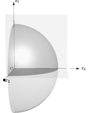
(a) Reflection with respect to $x_{3}=0$.

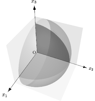
(b) Reflectiom with respect to $x_{3}=0$ and $x_{1}=0$.

Figure 2. Reflections of the localized problem.

By $\operatorname{supp}\zeta$ we denote the support of the cut-off function $\zeta$, and $\bar{v}$ denotes $v$ localized to $\operatorname{supp}\zeta$, i.e. $\bar{v}=v\zeta$. Similarly, since $f=0$ we immediately get that $\frac{\partial p}{\partial n}=0$ on each part of the boundary. This implies that the reflection with respect to $x_{3}$ preserves the Stokes system. Now, to get the problem in the half-space we need one more reflection (see Figure 2b). Observe that on $x_{1}=0$ we have $v_{1}=v_{2,x_{1}}=v_{3,x_{1}}=0$ and $\frac{\partial p}{\partial n}=0$, so we introduce

$$\check{\check{v}}(x)=\begin{cases}\check{v}(x)&x_{1}\in\overline{\operatorname{supp}\check{v}},\\ (-\check{v}_{1}(\bar{\bar{x}}),\check{v}_{2}(\bar{\bar{x}}),\check{v}_{3}(\bar{\bar{x}}))&x_{1}\leq 0,\end{cases}$$

where $\bar{\bar{x}}=(-x_{1},x_{2},x_{3})$. Now we see that $\check{\check{v}}$ is defined in the half-space $x_{2}\geq 0$ and the Stokes system is preserved.

Remark 4.2.

We have already mentioned that the assumption on the cubical shape of the domain can be relaxed. This motivation follows from (4.1), where the appearing boundary integral can be written in the form

(4.11) $$\int_{S}\sum_{i,j=1}^{3}v_{j,x_{i}}\cdot v_{j}\left\lvert v\right\rvert^{\theta-2}\cdot n_{i}\,\mathrm{d}S=\int_{S}\left\lvert v\right\rvert^{\theta-2}\left(\operatorname{rot}v\times n\right)\cdot v\,\mathrm{d}S-\int_{S}\sum_{i,j=1}^{3}v_{i,x_{j}}n_{i}v_{j}\,\mathrm{d}S.$$

We see that under (1.2) the first integral on the right-hand side vanishes.

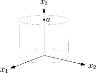
Figure 3. The set $\Omega$.

To eliminate the second integral we impose that $\Omega$ is of cylindrical type, parallel to the $x_{3}$ axis with convex cross section (see Figure 3). Denoting the side boundary by $S_{1}$, the bottom and the top of the cylinder (perpendicular to $x_{3}$) by $S_{2}$, the normal unit vector and the tangent unit vectors by $n$, $\tau^{\alpha}$, $\alpha=1,2$, respectively, we easily establish (see e.g. Introduction in [Zaj05a]) that

(4.12) $$n|_{S_{1}}=\frac{1}{\left\lvert\nabla\varphi\right\rvert}(\varphi_{,x_{1}},\varphi_{,x_{2}},0) \tau^{1}|_{S_{1}}=\frac{1}{\left\lvert\nabla\varphi\right\rvert}(-\varphi_{,x_{2}},\varphi_{,x_{1}},0) \tau^{2}|_{S_{1}}=(0,0,1)$$

$$n|_{S_{2}}=\left(0,0,\frac{a}{\left\lvert a\right\rvert}\right) \tau^{1}|_{S_{2}}=(1,0,0) \tau^{2}|_{S_{2}}=(0,1,0),$$

where $\varphi(x_{1},x_{2})=c_{0}$ is a sufficiently smooth, convex, closed curve in the plane $x_{3}=\operatorname{const}$.

Since $n$ does not depend on $x_{3}$ on $S_{1}$ we get in view of (4.12) that

$$\int_{S_{1}}\sum_{i,j=1}^{3}v_{i,x_{j}}n_{i}v_{j}\,\mathrm{d}S=\frac{\left(v\cdot\tau_{1}\right)^{2}}{\left\lvert\nabla\varphi\right\rvert^{3}}\left(\tau^{1}_{1}n_{1,x_{1}}\tau^{1}_{1}+\tau^{1}_{1}n_{1,x_{2}}\tau^{1}_{2}+\tau^{1}_{2}n_{2,x_{1}}\tau^{1}_{1}+\tau^{1}_{2}n_{2,x_{2}}\tau^{1}_{2}\right)=(v\cdot\tau_{1})^{2}\cdot\kappa,$$

where $\kappa$ is the curvature of $\varphi$. On $S_{2}$ we immediately see that $v_{3}=v_{3,x_{1}}=v_{3,x_{2}}=0$. Thus, (4.11) is negative and can be safely removed from (4.1).

For further geometrical considerations of the last term on the right-hand side in (4.11) we would refer the reader to e.g. [Wat03, Section 2].

Remark 4.3.

If we do not use the estimate for the pressure from Theorem 1, then we proceed as follows. First, we multiply (1.1)_1,2, (1.2) and (1.3) by $\eta_{k}(t)$, $k\in\mathbb{N}$, where

$$\eta_{k}(t)=\begin{cases}1&\text{for }t\in\big{(}kT,(k+1)T\big{)},\\ 0&\text{for }t\leq(k-1)T\end{cases}$$

with the properties $\eta_{k}\in\mathcal{C}^{\infty}_{c}(0,\infty)$ and $\frac{\mathrm{d}}{\mathrm{d}t}\eta_{k}(t)\leq\frac{1}{T}$. Denoting $\bar{v}=v\eta_{k}$ (we omit $k$ for clarity) we see that (1.1) becomes

(4.13) $$\bar{v}_{,t}+(v\cdot\nabla)\bar{v}-\nu\triangle\bar{v}+\nabla\bar{p}=\bar{f}-v\eta_{,t}=:\bar{F} \text{in $\Omega\times\big{(}(k-1)T,(k+1)T\big{)}=:\Omega^{kT}$},$$

$$\operatorname{div}\bar{v}=0 \text{in $\Omega^{kT}$},$$

$$v|_{t=(k-1)T}=0 \text{in $\Omega$}.$$

and for (1.2) and (1.3) we have

(4.14) $$\begin{aligned} &n\cdot\mathbb{D}(\bar{v})\cdot\tau_{\alpha}=0,\\ &n\cdot\bar{v}=0\end{aligned} \partial\Omega$$ on

and

(4.15) $$\begin{aligned} &\operatorname{rot}\bar{v}\times n=0,\\ &n\cdot\bar{v}=0\end{aligned} \partial\Omega$$ on .

By similar reasoning as in [Sol02] we get

$$\left\lVert\bar{v}\right\rVert_{W^{2,1}_{p,q}(\Omega^{kT})}+\left\lVert\nabla p\right\rVert_{L_{q}((k-1)T,(k+1)T;L_{p}(\Omega))}\\ \leq c(\nu,p,q,T,\Omega)\left(\left\lVert(v\cdot\nabla)\bar{v}\right\rVert_{L_{q}((k-1)T,(k+1)T;L_{p}(\Omega))}+\left\lVert\bar{F}\right\rVert_{L_{q}((k-1)T,(k+1)T;L_{p}(\Omega))}\right).$$

The Hölder inequality implies that

$$\left\lVert(v\cdot\nabla)\bar{v}\right\rVert_{L_{q}((k-1)T,(k+1)T;L_{p}(\Omega))}\leq\left\lVert v\right\rVert_{L_{s}((k-1)T,(k+1)T;L_{r}(\Omega))}\left\lVert\nabla\bar{v}\right\rVert_{L_{\beta}((k-1)T,(k+1)T;L_{\alpha}(\Omega))},$$

where

(4.16) $$\frac{1}{r}+\frac{1}{\alpha}=\frac{1}{p}\qquad\text{and}\qquad\frac{1}{s}+\frac{1}{\beta}=\frac{1}{q}.$$

The imbedding $W^{2,1}_{p,q}(\Omega^{kT})\hookrightarrow{L_{q}((k-1)T,(k+1)T;L_{p}(\Omega))}$ holds (see e.g. [BIN78, Ch.3, §10.2]) provided

$$\left(\frac{1}{p}-\frac{1}{\alpha}\right)\frac{3}{2}+\frac{1}{2}+\left(\frac{1}{q}-\frac{1}{\beta}\right)=1,$$

which in view of (4.16) is equivalent to

$$\frac{3}{r}+\frac{2}{s}=1.$$

Thus,

(4.17) $$\left\lVert\bar{v}\right\rVert_{W^{2,1}_{p,q}(\Omega^{kT})}+\left\lVert\nabla p\right\rVert_{L_{q}((k-1)T,(k+1)T;L_{p}(\Omega))}\\ \leq c(\nu,p,q,T,\Omega)\left(\left\lVert v\right\rVert_{L_{s}((k-1)T,(k+1)T;L_{r}(\Omega))}+\frac{c(initial\ data)}{T}+\left\lVert\bar{f}\right\rVert_{L_{q}((k-1)T,(k+1)T;L_{p}(\Omega))}\right)$$

for $T$ small enough.

By the same interpolation argument we deduce that the solution to (1.1) satisfies

$$\left\lVert v\right\rVert_{W^{2,1}_{p,q}(\Omega^{T})}+\left\lVert\nabla p\right\rVert_{L_{q}(0,T;L_{p}(\Omega))}\\ \leq c(\nu,p,q,T,\Omega)\left(\left\lVert v\right\rVert_{L_{s}(0,T;L_{r}(\Omega))}+\left\lVert f\right\rVert_{L_{q}(0,T;L_{p}(\Omega))}\right)+\left\lVert v(0)\right\rVert_{W^{2-\frac{2}{p}}(\Omega)}$$

for $T$ small enough. Thus, combining the above inequality with (4.17) and summing over $k$ yields

$$\left\lVert v\right\rVert_{W^{2,1}_{p,q}(\Omega^{T})}+\left\lVert\nabla p\right\rVert_{L_{q}(0,T;L_{p}(\Omega))}\leq c(initial\ and\ external\ data)$$

for arbitrary large $T<+\infty$. Now, the classical theory yields smoothness of $v$ and $p$.

References

- [AJ94] V. Adolfsson and D. Jerison, -integrability of the second order derivatives for the Neumann problem in convex domains, Indiana Univ. Math. J. 43 (1994), no. 4, 1123–1138.
- [BCJ08] H.-O. Bae, H.J. Choe, and B.J. Jin, Pressure representation and boundary regularity of the Navier-Stokes equations with slip boundary condition, J. Differential Equations 244 (2008), no. 11, 2741–2763.
- [Ber09] L.C. Berselli, Some criteria concerning the vorticity and the problem of global regularity for the 3D Navier-Stokes equations, Ann. Univ. Ferrara Sez. VII Sci. Mat. 55 (2009), no. 2, 209–224.
- [BG02] L.C. Berselli and G.P. Galdi, Regularity criteria involving the pressure for the weak solutions to the Navier-Stokes equations, Proc. Amer. Math. Soc. 130 (2002), no. 12, 3585–3595.
- [BIN78] O.V. Besov, V.P. Il’in, and S.M. Nikol’skiĭ, Integral representations of functions and imbedding theorems. Vol. I, V. H. Winston & Sons, Washington, D.C., 1978, Translated from the Russian, Scripta Series in Mathematics, Edited by Mitchell H. Taibleson.
- [BJ08] H.-O. Bae and B.J. Jin, Regularity for the Navier-Stokes equations with slip boundary condition, Proc. Amer. Math. Soc. 136 (2008), no. 7, 2439–2443.
- [BV11] C. Bjorland and A. Vasseur, Weak in space, log in time improvement of the Ladyženskaja-Prodi-Serrin criteria, J. Math. Fluid Mech. 13 (2011), no. 2, 259–269.
- [Cho98] H.J. Choe, Boundary regularity of weak solutions of the Navier-Stokes equations, J. Differential Equations 149 (1998), no. 2, 211–247.
- [CT08] C. Cao and E.S. Titi, Regularity criteria for the three-dimensional Navier-Stokes equations, Indiana Univ. Math. J. 57 (2008), no. 6, 2643–2661.
- [FKS09] R. Farwig, H. Kozono, and H. Sohr, Energy-based regularity criteria for the Navier-Stokes equations, J. Math. Fluid Mech. 11 (2009), no. 3, 428–442.
- [Gal00] G.P. Galdi, An introduction to the Navier-Stokes initial-boundary value problem, Fundamental directions in mathematical fluid mechanics, Adv. Math. Fluid Mech., Birkhäuser, Basel, 2000, pp. 1–70.
- [GKT06] S. Gustafson, K. Kang, and T.-P. Tsai, Regularity criteria for suitable weak solutions of the Navier-Stokes equations near the boundary, J. Differential Equations 226 (2006), no. 2, 594–618.
- [Gri85] P. Grisvard, Elliptic problems in nonsmooth domains, Monographs and Studies in Mathematics, vol. 24, Pitman (Advanced Publishing Program), Boston, MA, 1985.
- [Hop50] E. Hopf, Über die Anfangswertaufgabe für die hydrodynamischen Grundgleichungen., Math. Nachr. 4 (1950), no. 1, 213–231.
- [Kim10] J.-M. Kim, On regularity criteria of the Navier-Stokes equations in bounded domains, J. Math. Phys. 51 (2010), no. 5, 053102, 7.
- [KL06] Kyungkeun Kang and Jihoon Lee, On regularity criteria in conjunction with the pressure of Navier-Stokes equations, Int. Math. Res. Not. (2006), Art. ID 80762, 25. MR 2250016 (2007j:35159)
- [KS04] H. Kozono and Y. Shimada, Bilinear estimates in homogeneous Triebel-Lizorkin spaces and the Navier-Stokes equations, Math. Nachr. 276 (2004), 63–74.
- [KZ06] I. Kukavica and M. Ziane, One component regularity for the Navier-Stokes equations, Nonlinearity 19 (2006), no. 2, 453–469.
- [LSU67] O.A. Ladyženskaja, V.A. Solonnikov, and N.N. Ural’ceva, Linear and quasilinear equations of parabolic type, Translated from the Russian by S. Smith. Translations of Mathematical Monographs, Vol. 23, American Mathematical Society, Providence, R.I., 1967.
- [Maz09] V. Maz’ya, On the boundedness of first derivatives for solutions to the Neumann-Laplace problem in a convex domain, J. Math. Sci. (N. Y.) 159 (2009), no. 1, 104–112, Problems in mathematical analysis. No. 40.
- [Now13] B. Nowakowski, Large time existence of strong solutions to micropolar equations in cylindrical domains, Nonlinear Anal. Real World Appl. 14 (2013), no. 1, 635–660.
- [PP11] P. Penel and M. Pokorný, On anisotropic regularity criteria for the solutions to 3D Navier-Stokes equations, J. Math. Fluid Mech. 13 (2011), no. 3, 341–353.
- [Sol64] V. A. Solonnikov, Estimates for solutions of a non-stationary linearized system of Navier-Stokes equations, Trudy Mat. Inst. Steklov. 70 (1964), 213–317.
- [Sol76] by same author, Estimates of the solution of a certain initial-boundary value problem for a linear nonstationary system of Navier-Stokes equations, Zap. Naučn. Sem. Leningrad. Otdel Mat. Inst. Steklov. (LOMI) 59 (1976), 178–254, 257, Boundary value problems of mathematical physics and related questions in the theory of functions, 9.
- [Sol77] by same author, The solvability of the second initial-boundary value problem for a linear nonstationary system of Navier-Stokes equations, Zap. Naučn. Sem. Leningrad. Otdel. Mat. Inst. Steklov. (LOMI) 69 (1977), 200–218, 277, Boundary value problems of mathematical physics and related questions in the theory of functions, 10.
- [Sol90] by same author, An initial-boundary value problem for a Stokes system that arises in the study of a problem with a free boundary, Trudy Mat. Inst. Steklov. 188 (1990), 150–188, 192, Translated in Proc. Steklov Inst. Math. 1991, no. 3, 191–239, Boundary value problems of mathematical physics, 14 (Russian).
- [Sol02] by same author, Estimates of solutions of the Stokes equations in S. L. Sobolev spaces with a mixed norm, Zap. Nauchn. Sem. S.-Peterburg. Otdel. Mat. Inst. Steklov. (POMI) 288 (2002), no. Kraev. Zadachi Mat. Fiz. i Smezh. Vopr. Teor. Funkts. 32, 204–231, 273–274.
- [Str07] M. Struwe, On a Serrin-type regularity criterion for the Navier-Stokes equations in terms of the pressure, J. Math. Fluid Mech. 9 (2007), no. 2, 235–242.
- [Wat03] J. Watanabe, On incompressible viscous fluid flows with slip boundary conditions, Proceedings of the 6th Japan-China Joint Seminar on Numerical Mathematics (Tsukuba, 2002), vol. 159, 2003, pp. 161–172.
- [Zaj04] W.M. Zajączkowski, Global special regular solutions to the Navier-Stokes equations in a cylindrical domain under boundary slip conditions, GAKUTO International Series, Mathematical Sciences and Applications, no. 21, Gakkōtosho, 2004.
- [Zaj05a] by same author, Global regular nonstationary flow for the Navier-Stokes equations in a cylindrical pipe, Topol. Methods Nonlinear Anal. 26 (2005), no. 2, 221–286.
- [Zaj05b] by same author, Long time existence of regular solutions to navier-stokes equations in cylindrical domains under boundary slip conditions., Stud. Math. 169 (2005), no. 3, 243–285.
- [Zaj10] by same author, A regularity criterion for axially symmetric solutions to the Navier-Stokes equations, Zap. Nauchn. Sem. S.-Peterburg. Otdel. Mat. Inst. Steklov. (POMI) 385 (2010), no. Kraevye Zadachi Matematicheskoi Fiziki i Smezhnye Voprosy Teorii Funktsii. 41, 54–68, 234.
- [Zaj11] by same author, Nonstationary stokes system in Sobolev-Slobodetski spaces, Submitted.
- [Zho04] Y. Zhou, Regularity criteria in terms of pressure for the 3-D Navier-Stokes equations in a generic domain, Math. Ann. 328 (2004), no. 1-2, 173–192.
- [Zho06] by same author, On regularity criteria in terms of pressure for the Navier-Stokes equations in , Proc. Amer. Math. Soc. 134 (2006), no. 1, 149–156 (electronic).