Low stellar obliquities in compact multiplanet systems

Abstract

We measure the sky-projected stellar obliquities ($\lambda$) in the multiple-transiting planetary systems KOI-94 and Kepler-25, using the Rossiter-McLaughlin effect. In both cases the host stars are well-aligned with the orbital planes of the planets. For KOI-94 we find $\lambda=-11\pm 11^{\circ}$, confirming a recent result by Hirano and coworkers. Kepler-25 was a more challenging case because the transit depth is unusually small (0.13%). To obtain the obliquity it was necessary to use prior knowledge of the star’s projected rotation rate, and apply two different analysis methods to independent wavelength regions of the spectra. The two methods gave consistent results, $\lambda=7\pm 8^{\circ}$ and $-0.5\pm 5.7^{\circ}$.

There are now a total of five obliquity measurements for host stars of systems of multiple transiting planets, all of which are consistent with spin-orbit alignment. This alignment is unlikely to be the result of tidal interactions, because of the relatively large orbital distances and low planetary masses in the systems. In this respect the multiplanet host stars differ from hot-Jupiter host stars, which commonly have large spin-orbit misalignments whenever tidal interactions are weak. In particular the weak-tide subset of hot-Jupiter hosts have obliquities consistent with an isotropic distribution ($p=0.6$), but the multiplanet hosts are incompatible with such a distribution ($p\sim 10^{-6}$). This suggests that high obliquities are confined to hot-Jupiter systems, and provides further evidence that hot Jupiter formation involves processes that tilt the planetary orbit.

1. Introduction

Over the last few years, many stars with exoplanets have been found to have high obliquities, i.e., large angles between the stellar equator and the planet’s orbital plane (e.g. Hébrard et al., 2008; Winn et al., 2009; Queloz et al., 2010; Collier Cameron et al., 2010b; Moutou et al., 2011; Johnson et al., 2011; Albrecht et al., 2012b). However, for practical reasons almost all of the measurements have been made for stars with hot Jupiters. Systems with smaller planets, longer-period planets, and multiple planets remain relatively unexplored.

For the hot Jupiters, Winn et al. (2010) and Albrecht et al. (2012c) found evidence that the obliquities of many systems have been affected by tidal evolution: the systems for which one would expect planet-star tidal interactions to be strongest are preferentially found to have low obliquities. Systems with weaker tides have a more random obliquity distribution. This suggests that at the time of hot Jupiter formation, before tides had any opportunity to act, the orbital planes were only loosely correlated with the equatorial planes of their host stars. This in turn provides evidence that whatever “migration” process produces hot Jupiters also causes their orbits to be tilted away from the initial plane of formation, favoring scenarios such as planet-planet scattering or the Kozai effect over the once dominant paradigm of gradual inspiral within the protoplanetary disk.

The interpretation of the hot-Jupiter results is not settled, though, because the possibility remains that high obliquities are a generic feature of planetary systems, not specific to hot Jupiter migration. There are several proposed mechanisms for tilting a star relative to its protoplanetary disk: chaotic star formation (e.g. Bate et al., 2010; Thies et al., 2011), magnetic star-disk interactions (Lai et al., 2011; Foucart & Lai, 2011), torques due to internal gravity waves (Rogers et al., 2012), and torques due to neighboring stars Batygin (2012). In these scenarios, we should observe high obliquities not only in hot-Jupiter systems but also in a broader class of planetary systems.

One may test this idea by measuring stellar obliquities in systems with multiple transiting planets. In such systems the planets’ orbits are likely to be coplanar, and presumably mark the plane of the protoplanetary disk out of which the planets originally formed. If these systems have low stellar obliquities as a rule, then the high obliquities in hot-Jupiter systems are probably due to planet migration. If instead the obliquity distribution of multiple-transiting systems is similar to that of hot-Jupiter systems, then the obliquities are clues to more general processes in star and planet formation, and not specific to hot Jupiters.

The first multiple-transiting system for which the projected obliquity was measured was Kepler-30 (Sanchis-Ojeda et al., 2012). The authors took advantage of Kepler photometry and the occurrence of star-spots to measure the projected obliquity. More recently Hirano et al. (2012b) measured the projected obliquity in KOI-94 making use of the Rossiter-McLaughlin (RM) effect, and Chaplin et al. (2013) constrained the obliquities of Kepler-50 and Kepler-65 using asteroseismology. All of these systems were found to be consistent with good spin-orbit alignment.

Table 1Relative radial-velocity measurements

System	Time	RV	Unc.
	(BJDTDB)	(m s-1)	(m s-1)
Kepler-25	$2455761.77513$	$-7.07$	$3.53$
Kepler-25	$2455761.78302$	$-5.47$	$3.45$
Kepler-25	$2455761.85205$	$-6.80$	$3.77$
⋮

In this work we present an obliquity determination for the Kepler-25 multiple-transiting system, as well as an independent observation of the KOI-94 system. Between these and the previously published measurements, there are now five multiple-exoplanet systems for which we have information about the stellar obliquity (and of course the Solar system provides a sixth multiple-planet system). We are now in a position to make a statistical comparison between the multiple-planet systems and the hot-Jupiter systems.

The plan of this paper is as follows. The observations are described in Section 2. Section 3 presents the results for KOI-94. Section 4 gives the results for Kepler-25, which were obtained with two independent analysis methods because of the relatively challenging nature of the detection. The first method involved analyzing the “anomalous radial velocity” due to the RM effect (Section 4.1), and the second method involved direct modeling of the line-profile distortions (Section 4.2.4). As a test of the latter method, an analysis of archival spectra of the HAT-P-2 system is also presented. Finally, Section 5 presents statistical comparisons of the stellar obliquities in multiple-planet systems and hot-Jupiter systems.

2. Observations

All the observations analyzed here were obtained with the Keck I telescope and its High Resolution Spectrograph (HIRES; Vogt et al., 1994). We observed KOI-94 during the night of 2012 August 9/10, when it was transited by KOI-94.01. We observed Kepler-25 on two nights coinciding with transits of the largest planet c (2011 July 18/19 and 2012 May 31/June 1). We determined relative radial velocities in the usual way for HIRES, by analyzing the stellar spectra filtered through an iodine cell. The iodine absorption lines cover the wavelength range from about 500 to 600 nm. The analysis was performed with a descendant of the original code by Butler et al. (1996). The RVs of the Kepler-25 and KOI-94 systems are presented in Table 1.

3. KOI-94

The KOI-94 system has been studied in detail by Weiss et al. (2013). It harbors four planets in orbit around a late F-star (Table 2). KOI-94.01 is the largest of these planets, blocking nearly $0.8$% of the starlight during transits. By analyzing the light-curve of a mutual planet–planet eclipse in front of the stellar disk, Hirano et al. (2012b) showed that the mutual inclination between KOI-94.01 and KOI-94.03 is low ($1.15\pm 0.55^{\circ}$). This suggests that the planets have not been dynamically disrupted and that their orbits are faithful indicators of the plane of their formation.

Table 2Characteristics of KOI-94

KIC	6462863
Kepler magnitude	$12.2$
$T_{\rm eff}$	$6182(58)$ K
$\log g$	$4.182(0.066)$
Metallically, [Fe/H]	$0.0228(20)$
Projected stellar rotation speed, $v\sin i_{\star}$	$7.3(0.5)$ km s-1
Stellar radius, $R_{\star}$	$1.52(14)~{}R_{\odot}$
Stellar mass, $M_{\star}$	$1.277(50)~{}M_{\odot}$
$\star$ Data from MAST archive http://archive.stsci.edu/kepler/
$\dagger$ Data from Weiss et al. (2013)

Figure 1.— Rossiter-McLaughlin effect for KOI-94. Left: Apparent RV variation spanning the transit of planet KOI-94.01 on 2012 August 9/10. Black error bars show internal uncertainties as estimated by the RV measurement routine; gray error bars show uncertainties after adding a ’stellar jitter’ term in quadrature with the internal uncertainties to obtain a reduced $\chi^{2}$ of $1$. In the upper left panel, the solid curve represents the best-fitting model. The lower left panel displays the residuals, with the light and dark gray bars indicating the calculated times of first, second, third and fourth contact. Right panels: Parameter distributions, based on an MCMC analysis. The main plot shows the posterior in the $v\sin i_{\star}$ –$\lambda$ plane, with dark shading indicating high probability. The black, dark gray, and light gray lines outline the two-dimensional $68.3$ %, $95$ %, and $99.73$ % confidence limits. The one-dimensional projections of this posterior are shown on the upper and right sides. We find $\lambda=-11\pm 11^{\circ}$ and $v\sin i_{\star}$ $=7.3\pm 0.6$ km s^-1. The dashed line indicates the prior knowledge on $v\sin i_{\star}$  ($7.3\pm 1.5$ km s^-1) which was adopted for this analysis.

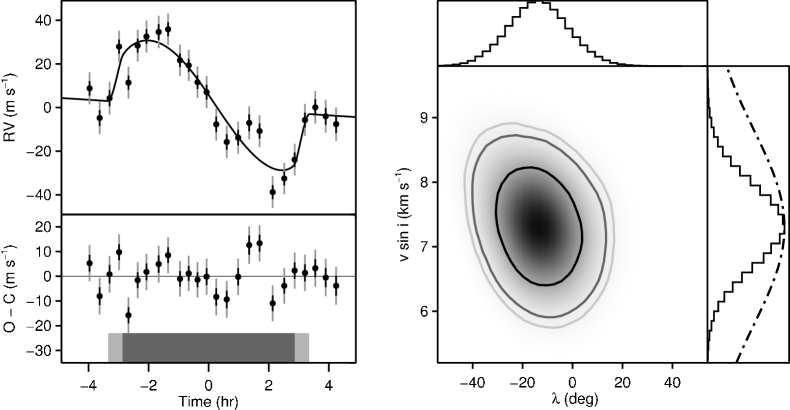
By observing the RM effect with Subaru and its High Dispersion Spectrograph, Hirano et al. (2012b) measured a low projected obliquity ($\lambda=-6_{+13}^{-11}$^∘) for the host star, relative to the orbit of KOI-94.01. Here, we present an analysis of the very same transit, based on data obtained with a different telescope. To analyze the RVs we used the approach of Albrecht et al. (2012c), which is based on the analytic description of the RM effect by Hirano et al. (2011) to model the RM effect. The model takes into account the rotation of the star, macroturbulence (e.g. Gray, 2005), thermal broadening, and line-broadening due to the finite resolution of the spectrograph. We added the prescription for the convective blueshift developed by Shporer & Brown (2011), as implemented by Albrecht et al. (2012b). We assumed the convective blueshift to have an amplitude of $1$ km s^-1, larger than that of the Sun ($0.5$ km s^-1) because it is thought that slightly hotter stars such as KOI-94 have stronger convective blueshifts (see Shporer & Brown, 2011, and references therein).

Along with the RVs, we analyzed the transit photometry obtained with the Kepler telescope in its short cadence mode (one-minute sampling). We fitted the photometric data with the Mandel & Agol (2002) transit model to determine the orbital period ($P$), the time of a particular mid-transit ($T_{\rm c}$), and the geometric parameters of the transit. The geometric parameters are the stellar radius in units of the orbital distance ($R_{\star}/a$), the planet-to-star radius ratio ($R_{\rm p}/R_{\star}$), and the cosine of the orbital inclination ($\cos i_{\rm o}$). We assumed a quadratic limb-darkening law and allowed both of the coefficients to be free parameters. The light curve was fitted simultaneously with the RVs. To calculate the anomalous RV due to the RM effect, we also assumed a quadratic limb-darkening law, with priors on the coefficients based on the tabulated values of Claret (2000): $u_{1,{\rm RM}}=0.35$ and $u_{2,{\rm RM}}=0.35$. We allowed ($u_{1,{\rm RM}}+u_{2,{\rm RM}}$) to be adjusted, with prior constraint centered on the tabulated value of $0.7$ and with a Gaussian width of $0.1$. The difference between the two parameters ($u_{1,{\rm RM}}-u_{2,{\rm RM}}$) was held fixed at the tabulated value of $0.0$ since the difference is only weakly constrained by the data and in turn has little effect on the other parameters.

Our prior on the projected stellar rotation speed ($v\sin i_{\star}$) was based on the determination by Weiss et al. (2013) using Spectroscopy Made Easy (SME; see Table 2). This spectroscopic modeling code is described by Valenti & Piskunov (1996); Valenti & Fischer (2005). Our confidence interval for this prior was enlarged to $1.5$ km s^-1, because the $v\sin i_{\star}$ value measured from the broadening of stellar absorption lines might not be fully representative for the projected rotation speed of the stellar surface area covered during transit. For example depending on the impact parameter, differential rotation might lead to such a mismatch. Our prior on the macroturbulent velocity is based on Valenti & Fischer (2005). From their equation (1) we obtained a macroturbulence velocity ($\zeta$) of $5.17$ km s^-1, for which we assumed a confidence interval of $1.5$ km s^-1.

To isolate the RM signal one must subtract (or model simultaneously) the orbital RV variation. One possibility is to subtract a model of the orbital RV variation based on the RV semiamplitude ($K_{\star}$) obtained by Weiss et al. (2013), which was based on RVs obtained sporadically over several months. We did not choose this approach out of concern that apparent RV variation due to starspots or other astrophysical noise can depend strongly on timescale. Starspot-induced signals, for example, can introduce slow drifts in the measured RV signal on a particular night. Such a signal would be averaged out in a data set obtained over many stellar rotation periods. See Albrecht et al. (2012c) for examples of this effect and how it can influence measurements of $\lambda$. Consequently we did not apply a prior constraint on $K_{\star}$ or on the systemic velocity $\gamma$ in our analysis.

For the estimation of the uncertainty intervals, we used an MCMC algorithm (see, e.g., Tegmark et al., 2004). In Table 3 we report the results derived from the posterior, where the quoted uncertainties exclude $15.85$ % of all values at both extremes, and encompass $68.3$ % of the total probability. Figure 1 presents the measured RVs, the best fitting model and the posterior in the $v\sin i_{\star}$ –$\lambda$ plane. The key result is $\lambda=-11\pm 11^{\circ}$, a low projected obliquity between the orbital angular momentum of KOI-94.01 and the angular momentum of the stellar rotation. Hirano et al. (2012b) found $\lambda=-6^{+13}_{-11}$^∘, which is consistent with our results. However, there were some differences in the methods of analysis. Hirano et al. (2012b) did not account for correlations between the uncertainty in $\lambda$ and the uncertainties in $T_{c}$, $R_{\star}/a$, $R_{\rm p}/R_{\star}$, $i_{\rm o}$, or $\zeta$; they did not model the convective blueshift; and they used RV observations obtained on different nights. For a fairer comparison we repeated the analysis of their RVs with the same constraints we applied to our own data. In this way we found $\lambda=-7\pm 17^{\circ}$ based on the Subaru dataset. We therefore conclude that two independent data sets support the finding of a low stellar obliquity in the KOI-94 system.

4. Kepler-25

The transiting objects in the Kepler-25 system were confirmed to be planets by Steffen et al. (2012), through the detection and interpretation of transit timing variations (TTV). The system was also recently analyzed by Lithwick et al. (2012), who measured masses of $7.13\pm 2.5$ $M_{\earth}$ and $13.1\pm 2.6$ $M_{\earth}$ for the two transiting planets b and c. (For comparison the mass of Neptune is $17.15$ $M_{\earth}$.) Table 4 gives the basic system parameters. Detection of the RM effect for this system is particularly challenging because the largest planet c blocks only 0.13% of the starlight. This leads to a low signal-to-noise ratio (S/N) detection of the RM effect. To gain more confidence in the results we employed two different techniques for measuring $\lambda$, relying on two different portions of the stellar spectrum. These two measurements are largely independent, although for both methods we use the Kepler photometry as supporting data. In the first technique (section 4.1), we analyze the RV time series which is derived from the iodine region of the spectrum. In the second technique (section 4.2.4) we do not analyze RVs; rather, we directly model the deformation of the stellar absorption lines. For this we use a method which we originally developed for the analysis of mutual events in eclipsing star systems (Albrecht et al., 2007, 2009, 2011a, 2012a). A similar approach has also been used by Collier Cameron et al. (2010a, b); Miller et al. (2010); Gandolfi et al. (2012) and Brown et al. (2012).

Table 3Parameters of the KOI-94 system

Parameter	Values
Parameters mainly derived from photometry
Mid-transit time $T_{\rm c}$ [BJDTDB$-$2 400 000]	$54965.74092$  $\pm$	$0.00014$
Period, $P$ [days]	$22.342971$  $\pm$	$0.000004$
Cosine orbital inclination KOI-94.01, $\cos i_{\rm o}$	$0.0112$  $\pm$	$0.0012$
Fractional stellar radius, $R_{\rm\star}/a$	$0.03807$  $\pm$	$0.0003$
Fractional planetary radius, $R_{\rm p}/R_{\star}$	$0.07019$  $\pm$	$0.00018$
$u_{1}+u_{2}$	$0.538$  $\pm$	$0.018$
$u_{1}-u_{2}$	$0.070$  $\pm$	$0.053$
Parameters mainly derived from RVs
Velocity offset, $\gamma$ [m s-1]	$-2.3$  $\pm$	$2.1$
Orbital semi-amplitude, K⋆ [m s-1]	$74$  $\pm$	$64$
$\sqrt{v\sin i_{\star}}\sin\lambda$ [${\sqrt{\rm km\,s^{-1}}}$]	$-0.527$  $\pm$	$0.53$
$\sqrt{v\sin i_{\star}}\cos\lambda$ [${\sqrt{\rm km\,s^{-1}}}$]	$2.60$  $\pm$	$0.14$
Macro turbulence parameter, $\zeta$ [km s-1]	$5.04$  $\pm$	$1.5$
$u_{1,{\rm RM}}+u_{2,{\rm RM}}$	$0.65$  $\pm$	$0.3$
Indirectly derived parameters
Orbital inclination KOI-94.01, $i_{\rm o}$ [∘]	$89.36$  $\pm$	$0.07$
Full duration, $T_{14}$ [hr]	$6.689$  $\pm$	$0.008$
Ingress or egress duration, $T_{12}$ [hr]	$0.477$  $\pm$	$0.009$
Projected stellar rotation speed, $v\sin i_{\star}$ [km s-1]	$7.3$  $\pm$	$0.6$
Projected spin-orbit angle, $\lambda$ [∘]	$-11$  $\pm$	$11$

4.1. Analyzing the RVs

The analyis of the Kepler-25 RV time series was similar to the analysis of the KOI-94 RV time series. Because for Keopler-25 we had RV measurements from two different transit nights, separated by nearly one year, we introduced for each night a different velocity offset ($\gamma$) and a different parameter to fit the out-of-transit velocity slope ($K_{\star}$). We used a prior on $v\sin i_{\star}$  based on an SME analysis (see Table 4). For $\zeta$ we used $4.85\pm 1.5$ km s^-1, which was obtained in the same way as for KOI-94. From the tables of Claret (2000) we obtained prior information on the limb-darkening coefficients ($u_{1,{\rm RM}}=0.33$ and $u_{2,{\rm RM}}=0.36$). As the expected RM signal has an amplitude of only a few m s^-1, the convective blueshift (CB) might have a significant influence on the observed RM signal (Shporer & Brown, 2011). Thus we allowed the CB parameter to vary, with only a weak prior of $1\pm 0.5$ km s^-1  instead of keeping it fixed as we did for KOI-94.

Because the planet shows TTVs we used a slightly different approach for incorporating the Kepler photometry into our analysis. First we examined the Kepler photometry for the two particular transits observed with HIRES, and derived midtransit times. From these we computed the ephemeris $T_{\rm c}=2455762.03086\pm 0.00050$ BJD and $P=12\fd 7203424\pm 0\fd 00003$ days. Second, we measured midtransit times for all the Kepler transits and used these to create a single, phase-folded, high-S/N transit light curve for Kepler-25 c. This light curve was then fitted together with the RVs, providing tight constraints on the geometric transit parameters.

Figure 2 shows the RVs from both nights, and the results for $v\sin i_{\star}$ and $\lambda$ based on an MCMC analysis of these RVs. The results are given in Table 5, second column. Our measurement of $\lambda=5\pm 8^{\circ}$ is consistent with alignment between the orbital plane of planet c and the stellar equator.

Table 4Kepler-25: Stellar characteristics

KOI	244
KIC	4349452
Kepler magnitude	$10.73$ mag
$T_{\rm eff}$	$6301(82)$K
$\log g$	$4.02(0.1)$
Metallically, [FeH]	$-0.10(4)$
Projected stellar rotation speed, $v\sin i_{\star}$ km s-1	$9.5(0.5)$
Stellar radius, $R_{\star}$	$1.36(13)R_{\odot}$
Stellar mass, $M_{\star}$	$1.22(6)M_{\odot}$
$\star$ Data from MAST archive http://archive.stsci.edu/kepler/
$\dagger$ Obtained using the SME package Valenti & Piskunov (1996)
$\ddagger$ Data from Steffen et al. (2012)

Figure 2.— Measured projected obliquity in Kepler-25 The same as Figure 1 but this time for the Kepler-25 system. The RV measurements from the two transit nights are indicated with solid (July 18/19, 2011) and open (May/June 31/1, 2012) symbols. We find $\lambda=5\pm 8^{\circ}$ and $v\sin i_{\star}$ $=8.5\pm 0.6$.

Figure 3.— RM signal for different obliquities. The plot shows the expected RM signal for a system like Kepler-25 during transit of planet c. The solid line shows the signal for the parameters printed in the second column of Table 5 but now with $\lambda=0^{\circ}$. The dashed and dashed dotted lines show the signals for $\lambda=90^{\circ}$ and $\lambda=-90^{\circ}$. The maximum amplitude of the aligned signal is smaller than for the strongly misaligned cases.

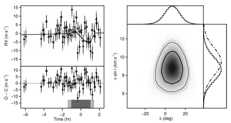
Because the amplitude of the RM effect is $\approx 4$ m s^-1, comparable to typical uncertainty of a single RV measurement, we must be skeptical and examine this result further. Why does our algorithm find such a small uncertainty interval for $\lambda$, given that the RM signal is so difficult to discern in the time series of the RV measurements (Figure 2)?

We have a great deal of prior knowledge of all the system parameters relevant for the RM effect, except for $\lambda$, allowing us to predict accurately the expected characteristics of the RM signal as a function of $\lambda$. To first order the amplitude of the RM effect is proportional to the covered surface area and the projected rotation speed. (See Gaudi & Winn, 2007; Albrecht et al., 2011b, for a more detailed discussion.) However the amplitude of the RM effect also depends on $\lambda$ itself. The amplitude of the RM signal is nearly twice as large for $\lambda=\pm 90^{\circ}$ as it is for $\lambda$ near $0^{\circ}$ or $180^{\circ}$ (Figure 3). Because of this and because there is a hint of a prograde signal in the RVs (Figure 2) the low projected obliquity is favored.

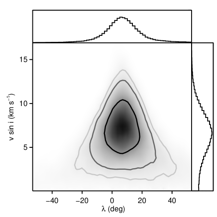
In more detail: we know from the Kepler photometry that planet c has a high impact parameter, i.e., it travels near the stellar limb throughout the transit. We also know a priori that the star has a substantial projected rotation speed from the SME analysis. Combining these two pieces of information we know there is no way to make the RM effect vanish. Figure 2 illustrates that we did not make a high-S/N detection of the RM effect. We might therefore ask which values of $\lambda$ would lead to the smallest RM amplitude, or an RM signal which would be easiest to hide by adjusting other parameters in our model. We have just noted that the maximum amplitude of the RM effect is larger for $|\lambda|$ near $90^{\circ}$ than for $\lambda$ near $0^{\circ}$ or $180^{\circ}$ (Figure 3). This is because limb darkening attenuates the signal by a factor of $0.6-0.7$ for a star like Kepler-25. The RM signal has maxima when the planet crosses the stellar limb where limb darkening is strongest, and the signal is zero near mid-transit where limb darkening is weakest. For $|\lambda|$ near $90$ degrees the maximum RM signal occurs nearer to the center of the stellar disk. In addition, the parameters $\gamma$ and $K_{\star}$ (the out-of-transit slope) are most strongly covariant with $\lambda$ when $\lambda$ is near $0^{\circ}$ or $180^{\circ}$ (Albrecht et al., 2011b). This is because of the time-antisymmetry of the RM signal in such cases. In contrast, for $\lambda$ near $\pm 90^{\circ}$ the RM signal is time-symmetric. Finally, differential rotation would also weaken the RM signal for $\lambda=0^{\circ}$ or $180^{\circ}$ compared to the $\lambda=\pm 90^{\circ}$ signal, though this is a comparatively minor effect ($\sim 10$ %). Together these factors make it easier to hide an RM signal with $\lambda=0$ (or $180$) than $\lambda=\pm 90^{\circ}$. Therefore, it is possible to infer that $\lambda$ must be near $0^{\circ}$ or $180^{\circ}$ with a sufficiently constraining upper limit on the amplitude of the RM effect. Here the data prefer $0^{\circ}$ over $180^{\circ}$ as there is a hint of a prograde RM signal in the data. As mentioned above there is only one parameter that is not at least partly constrained by photometry or prior knowledge, which is the projected obliquity. This is the qualitative explanation for the MCMC result of $\lambda=5\pm 8$ degrees. Note that the a priori knowledge on $v\sin i_{\star}$ is crucial in this situation (e.g Albrecht et al., 2011b). We illustrate this point by runing a chain without using the prior knowledge on $v\sin i_{\star}$ , where the uncertainty interval is enlarged to $\lambda=7\pm 13^{\circ}$. The result is shown in Figure 4.

However it is not completely satisfactory to argue for a low obliquity based on the absence of a clear signal. Therefore we sought an independent method to detect the RM effect. The next section describes our analysis of a wavelength region in which no iodine lines are present, and which therefore was not used in the determination of the RVs. We used this spectral range to make a second independent measurement of $\lambda$.

Figure 4.— Kepler-25 results without using prior knowledge on $v\sin i_{\star}$ . The same as the left panels from Figure 2 but this time without using the $v\sin i_{\star}$ prior. Constequently the uncertainties for $\lambda$ and $v\sin i_{\star}$ increased to $\lambda=7\pm 13^{\circ}$ and $v\sin i_{\star}$ $=6.2\pm 3$.

4.2. Measurement of the planet’s Doppler shadow

In this method of analysis we did not use RVs as proxies for the distortions in the stellar absorption lines. Instead we analyzed the line shapes directly to infer $\lambda$. The transiting planet selectively distorts the line profile, blocking a certain range of velocity components that ordinarily contribute to the overall line broadening, a phenomenon referred to as the “Doppler shadow” by Collier Cameron et al. (2010a). To model this phenomenon we used a code developed for double-lined eclipsing binaries (e.g. Albrecht et al., 2007, 2012a). For binary star systems, the difficulty lays in the additional set of stellar absorption lines originating from the eclipsing foreground star. In the case of planetary transits, this particular difficulty is eliminated, as the planet’s emitted light is negligible; rather, the challenge stems from the small amplitude of the RM signal. In the case of a Jupiter-sized planet such as HAT-P-2b, about 1% of the light is blocked from view. In the case of the transit of planet c in front of Kepler-25 only $0.13$ % of the light is blocked. For this reason we will present the application of our code to the Jupiter-sized planet in the bright ($m_{\rm V}=8.7$) HAT-P-2 system, as a test case. We then proceed to the more challenging Kepler-25 system.

4.2.1 The method

We used a two-step process to measure $\lambda$ from stellar spectra. In the first step we combined the signals from many stellar absorption lines into one high-S/N absorption line, which we will call the “kernel.” The spectrum is modeled as the convolution of the kernel and a series of $\delta$-functions at the central wavelengths of the absorption lines. This was done for each individual spectrum. In the second step, we analyzed the distortions that are seen in the kernels, which are caused by the transit of the planet over the rotating photosphere. As the first step is different from the approach used by Albrecht et al. (2007), we discuss it in detail in the following subsection.

Table 5Results for the Kepler-25 system.

Parameter	Values RV		Values Distortion
Parameters mainly derived from photometry
Mid-transit time $T_{\rm c}$ [BJDTDB$-$2 400 000]	$55762.0309$  $\pm$	$0.0005^{\rm a}$	$55762.0308$  $\pm$	$0.0005^{\rm a}$
Period, $P$ [days]	$12.72034$  $\pm$	$0.00003^{\rm a}$	12.7203424 (fixed)
Cosine orbital inclination Kepler-25 c, $\cos i_{\rm o}$	$0.0472$  $\pm$	$0.0008$	$0.0476$  $\pm$	$0.0008$
Fractional stellar radius, $R_{\rm\star}/a$	$0.0537$  $\pm$	$0.0007$	$0.0540$  $\pm$	$0.0007$
Fractional planetary radius, $R_{\rm p}/R_{\star}$	$0.0360$  $\pm$	$0.0006$	$0.0362$  $\pm$	$0.0007$
$u_{1}+u_{2}$	$0.569$  $\pm$	$0.020$	$0.560$  $\pm$	$0.019$
$u_{1}-u_{2}$	$-0.10$  $\pm$	$0.5$	$0.04$  $\pm$	$0.6$
Parameters mainly derived from spectroscopy
Velocity offset 2011, $\gamma$ [m s-1]	$-3.7$  $\pm$	$1.3$	b
Velocity offset 2012, $\gamma$ [m s-1]	$2.7$  $\pm$	$0.7$	b
Orbital semi-amplitude 2011, K⋆ [m s-1]	$-10$  $\pm$	$23$	b
Orbital semi-amplitude 2012, K⋆ [m s-1]	$-32$  $\pm$	$25$	b
$\sqrt{v\sin i_{\star}}\sin\lambda$ [${\sqrt{\rm km\,s^{-1}}}$]	$-0.35$  $\pm$	$0.39$	b
$\sqrt{v\sin i_{\star}}\cos\lambda$ [${\sqrt{\rm km\,s^{-1}}}$]	$2.9$  $\pm$	$0.23$	b
Macro turbulence parameter, $\zeta$ [km s-1]	$4.9$  $\pm$	$1.5$	$4.1$  $\pm$	$1.1$
Convective blueshift [km s-1]	$-1.0$  $\pm$	$0.5$	$-0.8$  $\pm$	$0.07$
$u_{1rm}+u_{2rm}$	$0.70$  $\pm$	$0.10$	$0.65$  $\pm$	$0.09$
Point Spread Function, PSF [km s-1]	3 (fixed)		$4.2$  $\pm$	$0.4$
Indirectly derived parameters
Impact parameter Kepler-25 c, $b$	$0.879$  $\pm$	$0.004$	$0.881$  $\pm$	$0.004$
Orbital inclination Kepler-25 c, $i_{\rm o}$ [∘]	$87.30$  $\pm$	$0.05$	$87.27$  $\pm$	$0.05$
Full duration, $T_{14}$ [hr]	$2.860$  $\pm$	$0.009$	$2.861$  $\pm$	$0.009$
Ingress or egress duration, $T_{12}$ [hr]	$0.405$  $\pm$	$0.014$	$0.410$  $\pm$	$0.015$
Projected stellar rotation speed, $v\sin i_{\star}$ [km s-1]	$8.7$  $\pm$	$1.3$	$8.2$  $\pm$	$0.2$c
Projected spin-orbit angle, $\lambda$ [∘]	$7$  $\pm$	$8$	$-0.5$  $\pm$	$5.7$c
Notes —
a We used the priors $P=12\fd 7203424\pm 0\fd 00003$  and $T_{\rm c}=2455762.03086\pm 0.00050$ BJD,
as determined using the Kepler photometry of the appropriate transits (see section  4.1).
b Was not determined.
c Here we step directly in $v\sin i_{\star}$ and $\lambda$ as they are less correlated than for RV measurements.

4.2.2 Measuring high S/N ratio stellar rotation kernels

Preparing the spectra.

The new algorithm works as follows. First we normalize the spectra using observations of fast rotating B-stars. Specifically we use polynomials fitted to the same and adjacent orders in the B-star spectrum to normalize the spectral orders of our science target. We use adjacent orders to remove the influence of shallow spectral lines present in the B star spectrum. All spectra are shifted according to the barycentric correction, and a correction term derived from the measurements of deep telluric lines in the red wavelength arm of HIRES. These corrections line up the spectra with an accuracy of $100-200$ m s^-1 (but see also below). Next, a high-S/N spectrum is created by averaging over all out-of-transit observations obtained during the night. Now each spectrum is compared to this high-S/N spectrum to mark and discard bad pixels. We also make one final small differential correction in the normalization of all spectra. For this we compare all spectra to the high-S/N spectrum and fit a third-order polynomial to the residuals, in which no absorption lines are present. Such a polynomial is created for each order and spectrum and is used for the correction.

Creating and refining a template.

To combine all the information contained in the different absorption lines, we need a sharp-lined template spectrum matching that of the target star. Our approach to obtain such a template—which matches the observed spectrum after convolution with a “master” absorption line profile—was inspired by Reiners & Schmitt (2003), but see also Donati et al. (1997) and Rucinski (1999) for similar approaches to obtain high-S/N kernels.

It is not only important that all the lines present in the observed spectrum are also present in the template; it is also important that the line depths in the template match the depths in the observed spectrum. We establish the appropriate line depths in the template spectrum in the following manner. As a starting point for this iterative process we query the Vienna Atomic Line Database (VALD; Kupka et al., 1999) for line positions and line depths appropriate for a star with the given effective temperature and surface gravity (our inputs in this case are based on the SME analysis; see Table 4). We now adjust the line depths so that a kernel convolved with the line list gives the best fit (smallest $\chi^{2}$) to the high-S/N spectrum we had obtained above. This kernel is created simultaneously with the optimization of the line depths. At this stage the kernel is purely phenomenological, and is not subject to any physical boundary conditions. It consists of a number of free parameters. Each parameter represents one pixel along the dispersion direction of the spectrograph, translated into velocity for the wavelength region of interest ($\approx 1.3$ km s^-1 at $390-480$ nm). The number of pixels is chosen such that the range of velocities that is covered is about twice as large as the $v\sin i_{\star}$ of the star. For HAT-P-2 we have $61$ free parameters and for Kepler-25 we have $33$ free parameters. To increase the speed of the computation each order is split into several sections, and for each section the best fitting line depths and kernels are found separately.

After this initial round we create an average kernel out of all kernels from all sections in all orders. Here the kernels from each section are weighted by the blaze function (for which we use the B-star spectra as proxy) of that section, and the equivalent width of the absorption lines in that section. We exclude regions at the short and long wavelength end of each order, regions dominated by deep, large lines, and regions for which clearly no good fit was achieved, i.e. lines are missing in the template. About 10% of the available spectral range was excluded for one or another of these reasons.

This newly obtained average kernel is now used for all sections in a second round, during which only line depths are adjusted. In the following round only the section kernels are optimized. These last two steps are repeated two more times to optimize the line depths. Finally the template with the optimized line depths is saved for later use, while the high-S/N spectrum as well as the average kernel are discarded.

Measuring high S/N ratio kernels.

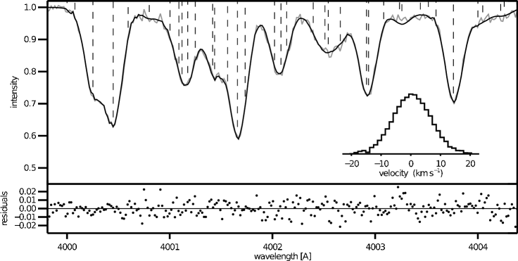
Now we use the depth-optimized template to obtain an average absorption line kernel in each section of all observations. Figure 5 displays one section of one Kepler-25 observation during the transit night. Also shown is the kernel derived from this section. Using the same weighting scheme as used above we can now create an average kernel for each observation.

4.2.3 Analyzing high-S/N kernels

The kernels obtained in the last section are then analyzed with the same code which was used by Albrecht et al. (2007). In short we pixelate the visible stellar surface and assign to each pixel a radial velocity, based on contributions from stellar rotation, macroturbulence, and the convective blueshift. At each phase of the transit we integrate over the exposed portion of the stellar surface to obtain the stellar absorption-line kernel. In this step we assume a quadratic limb-darkening law. Finally the absorption line is convolved with a Gaussian function representing both micro-turbulence in the photosphere and the point-spread function (PSF) of HIRES.

Changes in the spectrograph PSF during the transit nights.

Before the model absorption lines can be compared to the measured kernels one last step has to be taken which is specific to these observations. The spectra are obtained with a slit spectrograph and we therefore have to take into account possible changes in the PSF throughout the night. This is because small changes in telescope guiding cause variability in the illumination of the slit, and consequent changes in the PSF of the spectrograph. Changes in illumination of the slit might shift the PSF, sharpen or widen it, as well as introduce skewness and higher frequency terms. As a measured spectrum is convolved with the PSF such changes do effect the measured absorption lines directly.

We are interested in a time-varying signal: the distortion due to the transiting planet. Therefore it is important to compensate for changes in the absorption lines due to changes in the PSF. It is not crucial to know the PSF itself. In the next paragraph we explain how we deal with these potential shifts and stretches, and how we deal with higher-order changes by interpolating between observations obtained just before and after transit.

Figure 5.— Small portion of the normalized spectrum of Kepler-25. The thin gray line represents a small part of the third observed spectrum during the night of 2012 May 31/June 1. The dark line represents the convolution of the template (marked by the dashed lines) with the optimized kernel. The optimized kernel is shown in the lower right corner. The lower panel shows the difference between the observed spectrum and template convolved with the kernel. For each spectrum of Kepler-25, a total of about 900 Å were analyzed in the same fashion as shown in this 4 Å section.

To compensate for changes in the absorption lines caused by changes in the PSF we performed the following steps. We take the mean of the first few spectra, and the mean of the last few spectra, during a transit night. (If the PSF of the spectrograph would have been stable and our correction for any RV changes would have been perfect, then these should be identical, assuming no stellar activity). Next we linearly interpolate in time between these to create an absorption line appropriate for the time of each individual observation. These lines do not contain a transit signal, but include slow monotonic changes in the PSF. To isolate the transit signal we subtract the measured kernels from these interpolated lines.

Figure 6.— Doppler shadow of HAT-P-2b. During the planetary transit, part of the stellar photosphere is hidden from view, distorting the rotationally-broadened stellar absorption lines. The left upper panel (A) shows the time-variable planet shadow during a transit in the HAT-P-2 system. The dashed lines indicate times of first and last contact. At the beginning of the transit, parts of the approaching stellar surface area are hidden from view, and therefore blueshifted light is hidden. At the end of the transit, redshifted light is hidden. In addition to the transit signal, some artifacts are visible. They originate mainly form hour-to-hour (“fast”) changes in the wavelength position of the kernels. A mismatch in wavelength between the out-of-transit kernel and the current kernel leads to a deficit on one side of the kernel (dark) and a positive residual on the other side (light color). Panel (B) shows the results after correcting for these fast changes, as described in the text. Here, for illustration purposes, we only used an average kernel based on the post-transit data, rather than the interpolation between pre-transit and post-transit kernels, as described in the text. There is a continuous buildup of difference between the observed and assumed kernels towards the beginning of the night (“slow” changes). Panel (C) shows the results when the assumed kernel is based on interpolation in time between the pre-transit and post-transit kernels. Panel (D) shows the residuals after our best fitting model for the planetary transit is subtracted from the data shown in panel (C). There are some low-level patterns in the residuals, likely originating form changes in the PSF which are not modeled by our algorithm. To facilitate comparison between the different panels, the kernels form each system have been normalized to a height of unity (see Figure 7 and Figure 8). The grayscale bar next to each panel indicates the signal strength on the same scale. It is interesting to note that the depth of the HAT-P-2b velocity signal is more than twice as deep as the photometric transit signal. For rapidly rotating stars the depth of the deformation is not proportional to the square of the radii ratio, but is better approximated by the ratio itself.

Figure 7.— Doppler shadow of Kepler-25c. The same as panels (c) and (d) in Figure 6, but this time for the transit on 2012 May 31/June 1 of Kepler-25c. In the left panel (A) one can see the signature of a distortion traveling from negative RV towards positive RV throughout the transit: the signature of a prograde orbit. Modeling the distortion gives $\lambda=-0.5\pm 5.7^{\circ}$, indicating good alignment between the projections of the stellar and orbital spins. Panel (B) shows the residuals after subtraction of our best-fitting model.

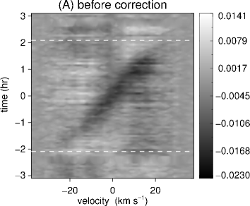
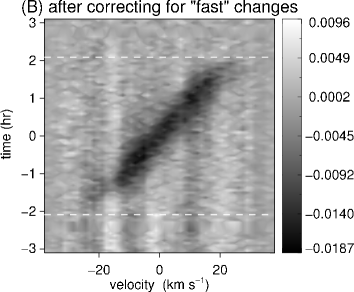
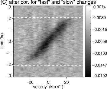
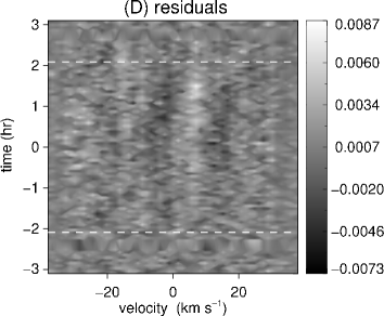
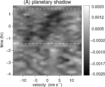
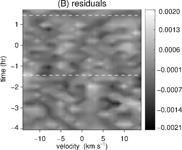
To correct for low-order fast changes in the PSF we allow the kernel of each observation to shift in velocity space and we further allow for a scaling in the velocity scale of the measured absorption line. This leads to two free parameters for each observation, which are evaluated each time the observations are compared to a specific model. The drifts are less then $200$ m s^-1 and the scaling in velocity space is always less than $0.5$ %. See Figure 6 for an illustration of how these different corrections influence the signal.

With this scheme we can compensate for a constant unknown PSF, slow changes in the PSF, as well as fast low-order changes in the PSF. We do not attempt to correct for fast high-order changes in the PSF as these would likely be correlated with the planet transit signal, which is itself a higher-order change in the stellar absorption lines.

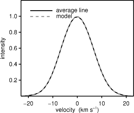
In addition to analyzing the changes in the absorption lines, we also use the observations taken before transit and compare them to the model line. This gives additional constraints on $v\sin i_{\star}$ , $\zeta$, and limb darkening. Here the PSF is modeled as a simple Gaussian with only one free parameter, the width ($\sigma_{\rm PSF}$). No accurate modeling of the PSF is required as we do not attempt to identify a small transit signal, but rather simply to measure the line width. See Figure 8 for a comparison between a measured absorption line and our model. The evaluation of the planet shadow and the out-of-transit line is done simultaneously.

Figure 8.— Comparison of overall line shape to model. The solid line shows the average line shape of Kepler-25 as measured with the first three observation during the transit May/June 31/1, 2012. The gray dashed line shows our best-fitting model of this line. The model includes quadratic limb-darkening, stellar rotation, micro and macroturbulence, the convective blueshift, and a PSF which is modeled as a simple Gaussian. Apart from the $\sigma_{\rm PSF}$ parameter, all other parameters are also simultaneously used to find the best-fitting model for the planet shadow (Figure 7). Our results for HAT-P-2 are not shown here but are of similar quality.

Figure 9.— Kepler-25 results form the analysis of the absorption lines and comparison to the RVs. The left panels show our results from the analysis of the distortion in the stellar absorption lines. We measure $\lambda=-0.5\pm 7^{\circ}$ and $v\sin i_{\star}=8.2\pm 0.2$ km s^-1. To allow a comparison to the RV data, the solid line in the right panel shows the anomalous RV signal that is implied by the best-fitting model of the line distortions. It is seen here to be compatible with the RV data even though the RV data was not used directly to constrain this model. (For this visual comparison, the out-of-transit RV trends were subtracted from the measured RVs.) The lower panel shows the difference between the measurements and the model, illustrating the good agreement between the line-distortion method and the anomalous-RV method for characterizing the planetary transit.

HAT-P-2

As our technique had to this point only been used for binary star systems, we applied it to the HAT-P-2 system before using it on the more challenging Kepler-25 dataset. The spectra of the HAT-P-2 system were obtained and analyzed by Winn et al. (2007) and the RVs were reanalyzed by Albrecht et al. (2012c) who found a low projected obliquity ($\lambda=9\pm 10^{\circ}$; the formal result was $\lambda=9\pm 5^{\circ}$, but due to residual structure in the RVs after substruction of our best fitting model we estimated the true uncertainty to be higher). Here we use the spectral region from $443$ to $455$ nm and the same photometric priors as used by Albrecht et al. (2012c). We find $\lambda=7.6\pm 0.5^{\circ}$. This is compatible with the RV-based results and, formally, implies a small misalignment in this system. However, given the patterned residuals visible in panel D of Figure 6 the true uncertainty is probably larger. To investigate this very high-S/N dataset further, the fidelity of our spectral model would need to be increased, and it would also be preferable to repeat the measurement with a different spectrograph. If the misalignment is confirmed than this would make HAT-P-2 an important system to study tidal alignment. Here, with the good agreement between the results of the RV and shape methods, we gained confidence that our algorithm to extract projected obliquities directly from modeling stellar absorption lines also works for the case of planetary transits observed with a slit spectrograph.

4.2.4 Kepler-25: changes in stellar absorption lines

Using the scheme described above we then analyzed the Kepler-25 spectra obtained during the two transit nights. We used the spectral region from $398$ to $479$ nm, blueward of the iodine lines. We did this separately for each transit night. We first focused on the transit night 2012 May 31/June 1. We used the same composite photometric light curve as used in our analysis of the RVs, and left $P$ fixed at the value determined from the photometry. With this method of analysis there is no need to determine $K_{\star}$ and $\gamma$ for the transit nights, as had been necessary for our analysis in Section 4.1. This reduced the number of free parameters by two; on the other hand there was a new parameter $\sigma_{\rm PSF}$ as described above. We did not impose any prior constraints on this parameter. To estimate the parameters and their uncertainty intervals we again used an MCMC algorithm.

Figure 10.— Changes in airmass during the Kepler-25 observations. The upper panel shows the changes in air-mass for the observations in 2011 (filled symbols) and 2012 (open symbols). The transit interval is indicated by the gray bars. Lower panel: The measured RVs for telluric lines on the red CCD of HIRES.

Figure 11.— Projected obliquity (either $\lambda$ or $i_{\star}$) as a function of the relative tidal-alignment timescale, for hot-Jupiter and multiple-planet systems. The systems are plotted as a function of a simple metric for the expected timescale for tidal dissipation within the star (see Albrecht et al. 2012c eq. 2–3). Stars which have temperatures higher then $6250$ K are shown with red filled symbols. Blue open symbols show stars with temperatures lower then $6250$ K. Stars which measured effective temperature include $6250$ K in their 1-$\sigma$ interval are shown by split symbols. Systems for which $\lambda$ was measured are indicated by a circle and refer to the left-hand axis. Measurements of $i_{\star}$ are indicated by a square and refer to the right-hand axis. Systems which harbor multiple planets are given dark black borders. The systems with short tidal timescales are seen to be well-aligned. All of the multiple-planet systems are well-aligned despite having weak tidal dissipation.

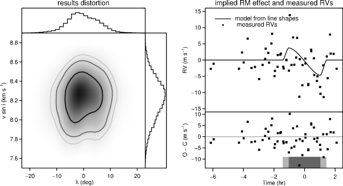
Figures 7 and 8 show the comparison between the data and the best-fitting models. Our results for $v\sin i_{\star}$  and $\lambda$ are shown in the left panel of Figure 9 and printed in column 3 of Table 5. These are consistent with the results found using the RVs of both data sets (Section 4.1, Table 5 column 2). In particular the results for $\lambda$ are consistent with each other. Analyzing RVs obtained with the iodine technique we obtain $\lambda=5\pm 8^{\circ}$. Analyzing the change in the absorption lines in the blue part of the spectrum we obtain $\lambda=-0.5\pm 5.7^{\circ}$. These results are independent from each other as different wavelength regions of the obtained spectra have been used (although the supporting photometric data was the same in both cases). In addition, the two independent measurements of $v\sin i_{\star}$ are consistent with each other. To illustrate the consistency of the results we show in the right panel of Figure 9 the expected RV signal from our best solution to the distortion of the absorption lines in the blue spectra. We further show the RVs measured during the two transits in the red part of the spectra, and which are displayed in Figure 2. We also show the difference between the measured RVs and the implied RV changes from the distortion. These signals are simply plotted on the same axes; they were not adjusted to match each other. The agreement of these two different approaches lends additional confidence to the conclusion that the projected stellar obliquity is low in Kepler-25. Why do we obtain a smaller uncertainty interval for $\lambda$ by measuring the deformations of the lines, rather than measuring RVs? We believe there are two reasons. When the line width is dominated by rotation, the spectroscopic transit depth is deeper than the broad-band transit, because in the spectroscopic transit only the portion of the star with the appropriate radial velocity is contributing to the contrast (Figure 7). Furthermore the $\lambda$ parameter is not strongly correlated with the other parameters that alter the position of the spectral lines, unlike the strong correlations that are observed when fitting RV data.

However, for the first transit night (2011 July 18/19) there was no secure detection of the Doppler shadow. What might have prevented a detection in this case? The main difference between the two datasets is a difference in the range of airmasses through which the observations were made (Figure 10, upper panel). During the 2011 transit the airmass increased from $1.1$ to $1.9$. In contrast, in 2012 the transit was observed at low zenith angles, always below an airmass of 1.1. The large variation in airmass during the 2011 observations strongly increases the difficulty of modeling the observed spectra. This is because a change in the angle under which an object is observed can lead to changes in the slit illumination which in turn changes the effective PSF. This can most readily be seen in the lower panel of Figure 10 where the apparent shift in radial velocity of telluric lines is plotted against time. The apparent changes are about $\approx 1$ km s^-1 for the night where we detect no signal and only $\approx 150$ m s^-1 where the changes in airmass are low and where the transit signal was detected. Telluric lines are intrinsically stable to at least a few tens of m s^-1 (e.g. Gray & Brown, 2006; Figueira et al., 2010).

The apparent changes in radial velocity of the telluric lines are measurement artifacts, caused by changes in the PSF, which also apply to stellar lines. We suspect that on top of the RV shifts higher order changes occur, which our algorithm cannot correct with sufficiently accuracy to allow for the detection of the small distortion induced by the planetary transit. During the observations of our test system HAT-P-2 the air-mass also changed significantly, from 1.2 to 2, and the observed RVs of telluric lines changed by $\approx 1$ km s^-1. The residuals of $0.8$ % in our test system (Figure 6, panel D) are larger than the expected distortion of $0.2$ % in the absorption lines in Kepler-25 (Figure 7, panel A). The signal of HAT-P-2b was nevertheless detected because of its relatively large amplitude; but the nondetection of a transit signal during the 2011 observations of Kepler-25 is not surprising in this context.

5. Comparison with Hot-Jupiter systems

In this section we will analyze our results for KOI-94 and Kepler-25 together with the results for three additional multi-transiting systems to try and clarify the interpretation of the high obliquities seen in hot-Jupiter systems. The other three systems are Kepler-30, 50, and 65. Using the occurrence of star spots, Sanchis-Ojeda et al. (2012) measured $\lambda$ to be $1\pm 10^{\circ}$ in Kepler-30. Chaplin et al. (2013) measured the inclination of the stellar rotation axis towards the observer ($i_{\star}$) for two additional systems, via asteroseismology. For Kepler-50 they found $i_{\star}=82^{+8}_{-7}$^∘ and for Kepler-65 they found $i_{\star}=81^{+9}_{-16}$^∘. An estimate of the stellar inclination in Kepler-50 had also been obtained earlier by Hirano et al. (2012a), using a combination of estimates for the rotation period, stellar radius, and $v\sin i_{\star}$. Their result was less constraining than, but compatible with, the result of Chaplin et al. (2013).

High obliquities: planet migration or star-disk evolution?

For HJ systems, evidence has accumulated that the stellar obliquities varied over a very large range when the gas giants arrived near their host stars (Winn et al., 2010; Schlaufman, 2010; Albrecht et al., 2012c). This has been taken as evidence that the orbital plane of the planet has changed, presumably via the same mechanism which also changed its orbital distance. However, as mentioned in the introduction, there are other mechanisms which might create a misalignment between the stellar orientation and the planetary orbit. In multiple-transiting planet systems there is reason to think that the orbits still trace the plane of the disk out of which they have formed. Therefore measuring the obliquities in these systems lets us learn about the degree of alignment between protoplanetary disks and stellar spin axes.

If we find that the distribution of obliquities for multiplanet systems is closer to alignment, than the distribution of obliquities for HJ systems, then this would indicate that the large obliquities in HJ systems are caused by the evolution of the planets’ orbits. If on the other hand we find that the distribution in obliquities for multiplanet systems is similar to the distribution of obliquities for HJs then the measured obliquities are not necessarily related to planet migration.

We note that the host stars in both groups, close in gas giants and multiple planet systems, are on the main-sequence and cover the spectral classes from F to K. The only readily apparent difference between these systems is that for one group, several planets are found on compact coplanar orbits, within in the other group there are solitary transiting gas giants.

The influence of tides.

Before we can compare the two distributions of obliquities we first need to know if tides have dampened the obliquities. It would be advantageous to only include systems which have not undergone any significant tidal influence, instead of attempting to model the influence of tides on the obliquity.

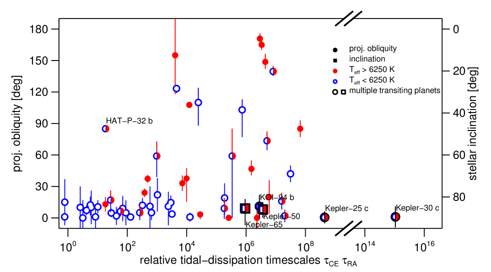
To check which systems might be influenced by tides, we calculate the same two alignment timescales presented in Albrecht et al. (2012c) for the multiple planet systems. Either approach to calculating the timescale leads to the conclusion that tides probably had little or no influence on the stellar obliquities in the five multiplanet systems. In Figure 11 we show the results for the timescale which is calibrated based on binary-star data (Albrecht et al., 2012c). In the same Figure we also show all the hot-Jupiter systems from Albrecht et al. (2012c), after including some newly published measurements. We included the new measurements for WASP-32 and WASP-38 from Brown et al. (2012), HAT-P-17 Fulton et al. (2013), updated the value for CoRoT-11 from Gandolfi et al. (2012), and updated the value for WASP-19 from Tregloan-Reed et al. (2013). As mentioned we also added the $\lambda$ and $i_{\star}$ measurements for the multiple transiting planet systems. The left-hand $y$-axis indicates $\lambda$ and the right-hand $y$-axis indicates $i_{\star}$. Indication of good alignment is a low value in $\lambda$ or a large value of $i_{\star}$. The long tidal realignment timescales in the studied multiple planet systems is due to the long orbital periods and the small masses of the planets.

According to Figure 11 it does seem unlikely that any of the multiple planet system was influenced by tides. But which hot Jupiter systems should be included in the comparison? As we do not have a clear cut criterion we will use three samples: (1) All hot Jupiters; (2) all hot Jupiters with $\tau$ equal or larger to the $\tau$ of the first clearly misaligned system ($\tau>10^{2.7}$); and (3) only hot Jupiters which have timescales $\tau$ equal to or larger than the shortest $\tau$ found amongst the multiple-planet systems ($\tau=10^{5.8}$).

Comparing the distributions.

In the regime of weak tides, the hot Jupiter results appear to be nearly random. Therefore we first ask: could either population be drawn from an isotropic distribution on a sphere? For hot Jupiters we have only measurements of $\lambda$, the projected obliquity. We can therefore compare these measurements to a distribution in $\lambda$ for the isotropic case using a Kolmogorov-Smirnov (K-S) test (e.g Press et al., 1992). For case (1) the K-S test suggests that there is negligible probability that the $\lambda$ measurements of all hot-Jupiter systems are drawn from an isotropic distribution. For case (2) there is still only a $0.04$ % probability that the results are drawn from an isotropic distribution. However for case (3) we find there is a $61$ % chance that this distribution is consistent with an isotropic distribution in $\lambda$. Figure 12 shows the cumulative distribution in $\lambda$ for these HJs and the expected distribution in $\lambda$ for an isotropic distribution.

For the multiple planet systems we have two distinct measures of obliquity, $\lambda$ and $i_{\star}$, which cannot be translated into each other (at least not without already assuming a distribution, see Fabrycky & Winn 2009). Therefore we use a Monte Carlo approach instead of a K-S test. We create a distribution of obliquities which has a uniform distribution in $\lambda$ (Kepler-30, KOI-94, Kepler-25) and in $\cos i_{\star}$ (Kepler-50, Kepler-65) to simulate a isotropic distribution in the obliquities. Form these we draw five “measurements” which we compare to the three measurements of $\lambda$ and two measurements of $i_{\star}$. The uncertainties in the actual measurements are included as Gaussian random numbers, every time a comparison is made. In particular for the comparison in $i_{\star}$ we use half-Gaussians with peaks at $90^{\circ}$ and standard deviations derived from the inclination measurement plus the measurement uncertainty. We repeat this experiment $5\times 10^{7}$ times. Only in $0.0003$% of these experiments do we draw sufficiently low values of $\lambda$, and sufficiently high values of $i_{\star}$, to be compatible with the measured $\lambda$s and $i_{\star}$. It seems unlikely that obliquities in multiple planet systems are drawn from an isotropic distribution. A narrow distribution centered near zero obliquity is more appropriate. We will defer an analysis of which is the exact distribution until more obliquity measurements in multiplanet systems are available. See Fabrycky & Winn (2009) for possible approaches on how a comparison can be made. Such an analysis would be interesting as it might shed light on the origin of the small ($6^{\circ}$) obliquity of the Sun.

Now combining that 1) multiplanet systems have a different obliquity distribution than systems with single, close-in gas giants, 2) planets in multiple planet systems presumably trace with their orbits the plane of the circumstellar disk out of which they formed, and 3) we are not able to detect any other significant difference between stars which have close in giant planets and stars which hosts multiple planets, we conclude that the misalignments between stellar rotation and planetary orbits are due to changes of the inclinations of the orbital planes. Our results disfavor theories which aim to explain large obliquities due to a change in the angle between protoplanetary disk and the star (e.g. Bate et al., 2010; Thies et al., 2011; Batygin, 2012) or changes in the internal structure of the star (Rogers et al., 2012).

Of course it must be acknowledged that a sample of 5 systems is not sufficient for a firm conclusion. The systems studied here only cover a small parameter space, for example a limited range in stellar mass. In other systems, mechanisms for tilting stars may be more important. One clue that this is indeed the case is the finding that both stars in the DI Herculis system are strongly inclined with respect to their mutual orbit (Albrecht et al., 2009). Here however, we have found that the evidence to date supports the conclusion that the high obliquities of hot-Jupiter systems are due to evolution of the planets’ orbits.

Figure 12.— Kolmogorov-Smirnov test on the isotropic distribution of $\lambda$ for single, close in, gas giant planets. The solid line shows the cumulative fraction of $|\lambda|$ for an isotropic distribution of obliquities on a sphere, all $\lambda$ are equally likely a priori. The dashed line shows the cumulative distribution for measurements of $\lambda$ in HJ systems. We only included systems with $\tau>10^{5.8}$ (See Figure 11), to avoid systems which are strongly influenced by tides. According to the Kolmogorov-Smirnov test there is a $61$% chance that the projected obliquities of these systems are drawn from an isotropic distribution.

Relation to planet migration theories.

If we assume that the smaller mass planets in multiple-planet systems migrated inwards then it seems that we have (at least) two types of processes which may be of importance in planet migration. One type of process changes the obliquity while the other does not. We could identify disk migration with the latter, and dynamical interactions with the former. We note, though, that it is not necessarily true that the compact multiplanet systems have experienced inward migration; see, for example, Chiang & Laughlin 2012.

A number of mechanisms have been proposed for changing the orbital inclination of a planet. Two processes which have attracted particular attention are planet-planet scattering (e.g. Rasio & Ford, 1996; Chatterjee et al., 2008; Matsumura et al., 2010; Nagasawa & Ida, 2011) and Kozai Cycles with Tidal Friction (KCTF, Eggleton & Kiseleva-Eggleton 2001). Kozai cycles can be induced by the influence of a distant stellar companion (e.g. Wu & Murray, 2003; Fabrycky & Tremaine, 2007; Naoz et al., 2012) or by a distant planet (e.g. Naoz et al., 2011). To confirm Kozai migration via a stellar companion, searches for stellar companions to hot-Jupiter hosts will be helpful (e.g. Narita et al., 2012). Another way to test theories of hot Jupiters involving tidal circularization from a highly eccentric orbit is to search for their putative high-eccentricity progenitors. Socrates et al. (2012) predicted that there should be a stream of gas giant on very eccentric orbits (eccentricity $<0.9$) if hot Jupiters were transported directly inwards from beyond the snow line. Dawson et al. (2012) searched the Kepler database for such objects, did not find any, and placed an upper bound on such a population. This indicates that if KCTF is an important migration path, then likely the starting point for KCTF is closer than the snow line. This suggests that gas giants migrate via a combination of processes. For example initial scattering or disk migration followed by Kozai cycles and finally tidal circularization.

6. Summary

In the multiple-planet systems KOI-94 and Kepler-25 we measured good alignment between the stellar rotation axes and the orbital plane of the transiting planets. For both systems we used the radial velocity anomaly (Rossiter-McLaughlin effect) during planetary transits to determine the degree of alignment. For KOI-94 our result is consistent with an independent study by Hirano et al. (2012b). As the Rossiter-McLaughlin effect in the Kepler-25 system has only a small amplitude, we further measured the distortion of the stellar absorption lines directly in another part of the obtained stellar spectra. We found consistent results with both methods.

Combining our results with measurements in three other multiple planet systems (Kepler-30, Kepler-50, Kepler-65) we can now compare the obliquity distributions of multiple planet systems to the obliquities measured in Hot-Jupiter systems. We find that there is only a $0.0003$ % chance that multiple planet systems have a isotropic obliquity distribution. This is in contrast to the apparent isotropic obliquity distribution in Hot-Jupiter systems when taking tidal realignment into account (i.e., omitting systems with relatively strong tidal interactions).

Our results support the idea that the inward migration of close in gas-giants is fundamentally different from the migration occurring in compact multiple planet systems. It suggests that the planets we see in the multiple planet systems might have migrated via disk-planet interactions while Hot-Jupiters must have taken a different route. Their path not only brought them close to their host stars but also transported them out of the orbital plane of the disk out in which they have formed.

References

- Albrecht et al. (2009) Albrecht, S., Reffert, S., Snellen, I. A. G., & Winn, J. N. 2009, Nature, 461, 373
- Albrecht et al. (2007) Albrecht, S., Reffert, S., Snellen, I., Quirrenbach, A., & Mitchell, D. S. 2007, A&A, 474, 565
- Albrecht et al. (2012a) Albrecht, S., Setiawan, J., Torres, G., Fabrycky, D. C., & Winn, J. N. 2012a, ArXiv e-prints, arXiv:1211.7065 [astro-ph.SR]
- Albrecht et al. (2012b) Albrecht, S., Winn, J. N., Butler, R. P., et al. 2012b, ApJ, 744, 189
- Albrecht et al. (2011a) Albrecht, S., Winn, J. N., Carter, J. A., Snellen, I. A. G., & de Mooij, E. J. W. 2011a, ApJ, 726, 68
- Albrecht et al. (2011b) Albrecht, S., Winn, J. N., Johnson, J. A., et al. 2011b, ApJ, 738, 50
- Albrecht et al. (2012c) —. 2012c, ApJ, 757, 18
- Bate et al. (2010) Bate, M. R., Lodato, G., & Pringle, J. E. 2010, MNRAS, 401, 1505
- Batygin (2012) Batygin, K. 2012, Nature
- Brown et al. (2012) Brown, D. J. A., Cameron, A. C., Anderson, D. R., et al. 2012, MNRAS, 423, 1503
- Butler et al. (1996) Butler, R. P., Marcy, G. W., Williams, E., et al. 1996, PASP, 108, 500
- Chaplin et al. (2013) Chaplin, W. J., Sanchis-Ojeda, R., Campante, T. L., et al. 2013, ApJ submitted
- Chatterjee et al. (2008) Chatterjee, S., Ford, E. B., Matsumura, S., & Rasio, F. A. 2008, ApJ, 686, 580
- Chiang & Laughlin (2012) Chiang, E., & Laughlin, G. 2012, ArXiv e-prints, arXiv:1211.1673 [astro-ph.EP]
- Claret (2000) Claret, A. 2000, A&A, 363, 1081
- Collier Cameron et al. (2010a) Collier Cameron, A., Bruce, V. A., Miller, G. R. M., Triaud, A. H. M. J., & Queloz, D. 2010a, MNRAS, 403, 151
- Collier Cameron et al. (2010b) Collier Cameron, A., Guenther, E., Smalley, B., et al. 2010b, MNRAS, 407, 507
- Dawson et al. (2012) Dawson, R. I., Murray-Clay, R. A., & Johnson, J. A. 2012, ArXiv, arXiv:1211.0554 [astro-ph.EP]
- Donati et al. (1997) Donati, J.-F., Semel, M., Carter, B. D., Rees, D. E., & Collier Cameron, A. 1997, MNRAS, 291, 658
- Eggleton & Kiseleva-Eggleton (2001) Eggleton, P. P., & Kiseleva-Eggleton, L. 2001, ApJ, 562, 1012
- Fabrycky & Winn (2009) Fabrycky, D. C., & Winn, J. N. 2009, ApJ, 696, 1230
- Fabrycky & Tremaine (2007) Fabrycky, D., & Tremaine, S. 2007, ApJ, 669, 1298
- Figueira et al. (2010) Figueira, P., Pepe, F., Lovis, C., & Mayor, M. 2010, A&A, 515, A106
- Foucart & Lai (2011) Foucart, F., & Lai, D. 2011, MNRAS, 412, 2799
- Fulton et al. (2013) Fulton, B. J., Howard, A. W., Winn, J. N., et al. 2013, ArXiv e-prints, arXiv:1301.6289 [astro-ph.EP]
- Gandolfi et al. (2012) Gandolfi, D., Collier Cameron, A., Endl, M., et al. 2012, A&A, 543, L5
- Gaudi & Winn (2007) Gaudi, B. S., & Winn, J. N. 2007, ApJ, 655, 550
- Gray (1984) Gray, D. F. 1984, ApJ, 281, 719
- Gray (2005) —. 2005, The Observation and Analysis of Stellar Photospheres, 3rd Ed. (ISBN 0521851866, Cambridge University Press)
- Gray & Brown (2006) Gray, D. F., & Brown, K. I. T. 2006, PASP, 118, 399
- Hébrard et al. (2008) Hébrard, G., Bouchy, F., Pont, F., et al. 2008, A&A, 488, 763
- Hébrard et al. (2013) Hébrard, G., Collier Cameron, A., Brown, D. J. A., et al. 2013, A&A, 549, A134
- Hirano et al. (2011) Hirano, T., Narita, N., Shporer, A., et al. 2011, PASJ, 63, 531
- Hirano et al. (2012a) Hirano, T., Sanchis-Ojeda, R., Takeda, Y., et al. 2012a, ApJ, 756, 66
- Hirano et al. (2012b) Hirano, T., Narita, N., Sato, B., et al. 2012b, ArXiv, arXiv:1209.4362 [astro-ph.EP]
- Isaacson & Fischer (2010) Isaacson, H., & Fischer, D. 2010, ApJ, 725, 875
- Johnson et al. (2011) Johnson, J. A., Winn, J. N., Bakos, G. Á., et al. 2011, ApJ, 735, 24
- Kupka et al. (1999) Kupka, F., Piskunov, N., Ryabchikova, T. A., Stempels, H. C., & Weiss, W. W. 1999, A&AS, 138, 119
- Lai et al. (2011) Lai, D., Foucart, F., & Lin, D. N. C. 2011, MNRAS, 412, 2790
- Lithwick et al. (2012) Lithwick, Y., Xie, J., & Wu, Y. 2012, ArXiv, arXiv:1207.4192 [astro-ph.EP]
- Mandel & Agol (2002) Mandel, K., & Agol, E. 2002, ApJ, 580, L171
- Matsumura et al. (2010) Matsumura, S., Peale, S. J., & Rasio, F. A. 2010, ApJ, 725, 1995
- Miller et al. (2010) Miller, G. R. M., Collier Cameron, A., Simpson, E. K., et al. 2010, A&A, 523, A52
- Moutou et al. (2011) Moutou, C., Díaz, R. F., Udry, S., et al. 2011, A&A, 533, A113
- Nagasawa & Ida (2011) Nagasawa, M., & Ida, S. 2011, ApJ, 742, 72
- Naoz et al. (2011) Naoz, S., Farr, W. M., Lithwick, Y., Rasio, F. A., & Teyssandier, J. 2011, Nature, 473, 187
- Naoz et al. (2012) Naoz, S., Farr, W. M., & Rasio, F. A. 2012, ApJ, 754, L36
- Narita et al. (2012) Narita, N., Takahashi, Y. H., Kuzuhara, M., et al. 2012, ArXiv, arXiv:1209.4422 [astro-ph.EP]
- Press et al. (1992) Press, W. H., Teukolsky, S. A., Vetterling, W. T., & Flannery, B. P. 1992, Numerical recipes in FORTRAN. The art of scientific computing, 2rd Ed. (Cambridge: University Press)
- Queloz et al. (2010) Queloz, D., Anderson, D., Collier Cameron, A., et al. 2010, A&A, 517, L1
- Rasio & Ford (1996) Rasio, F. A., & Ford, E. B. 1996, Science, 274, 954
- Reiners & Schmitt (2003) Reiners, A., & Schmitt, J. H. M. M. 2003, A&A, 398, 647
- Rogers et al. (2012) Rogers, T. M., Lin, D. N. C., & Lau, H. H. B. 2012, ArXiv, arXiv:1209.2435 [astro-ph.SR]
- Rucinski (1999) Rucinski, S. 1999, in ASP Conf. Ser. 185: IAU Colloq. 170: Precise Stellar Radial Velocities, ed. J. B. Hearnshaw & C. D. Scarfe, 82
- Sanchis-Ojeda et al. (2012) Sanchis-Ojeda, R., Fabrycky, D. C., Winn, J. N., et al. 2012, Nature, 487, 449
- Schlaufman (2010) Schlaufman, K. C. 2010, ApJ, 719, 602
- Shporer & Brown (2011) Shporer, A., & Brown, T. 2011, ApJ, 733, 30
- Socrates et al. (2012) Socrates, A., Katz, B., Dong, S., & Tremaine, S. 2012, ApJ, 750, 106
- Steffen et al. (2012) Steffen, J. H., Fabrycky, D. C., Ford, E. B., et al. 2012, MNRAS, 421, 2342
- Tegmark et al. (2004) Tegmark, M., Strauss, M. A., Blanton, M. R., et al. 2004, Phys. Rev. D, 69, 103501
- Thies et al. (2011) Thies, I., Kroupa, P., Goodwin, S. P., Stamatellos, D., & Whitworth, A. P. 2011, MNRAS, 417, 1817
- Tregloan-Reed et al. (2013) Tregloan-Reed, J., Southworth, J., & Tappert, C. 2013, MNRAS, 428, 3671
- Valenti & Fischer (2005) Valenti, J. A., & Fischer, D. A. 2005, ApJS, 159, 141
- Valenti & Piskunov (1996) Valenti, J. A., & Piskunov, N. 1996, A&AS, 118, 595
- Vogt et al. (1994) Vogt, S. S., Allen, S. L., Bigelow, B. C., et al. 1994, in SPIE Conference Series, ed. D. L. Crawford & E. R. Craine, Vol. 2198, 362
- Weiss et al. (2013) Weiss, L. M., Marcy, G. W., Rowe, J. F., et al. 2013, ApJ submitted
- Winn et al. (2010) Winn, J. N., Fabrycky, D., Albrecht, S., & Johnson, J. A. 2010, ApJ, 718, L145
- Winn et al. (2009) Winn, J. N., Johnson, J. A., Albrecht, S., et al. 2009, ApJ, 703, L99
- Winn et al. (2007) Winn, J. N., Johnson, J. A., Peek, K. M. G., et al. 2007, ApJ, 665, L167
- Wu & Murray (2003) Wu, Y., & Murray, N. 2003, ApJ, 589, 605