Deep redshift topological lensing: strategies for the $T^{3}$ candidate

Abstract

The 3-torus ($T^{3}$) Friedmann-Lemaître-Robertson-Walker (FLRW) model better fits the nearly zero large-scale two-point auto-correlation of the Wilkinson Microwave Anisotropy Probe (WMAP) cosmic microwave background (CMB) sky maps than the infinite flat model. The $T^{3}$ model’s parameters, recently found using an optimal cross-correlation method on WMAP data, imply approximately equal-redshift topological lensing at redshifts $z\sim 6$, the redshift range of the upcoming generation of new instruments and telescopes. We investigate observational strategies that can reject the $T^{3}$ solution for a given region of parameter space of physical assumptions, or provide good candidate topologically lensed galaxy pairs for detailed spectroscopic followup. $T^{3}$ holonomies are applied to (i) existing $z\sim 6$ observations and (ii) simulated observations, creating multiply connected catalogues. Corresponding simply connected catalogues are generated. The simulated observational strategies are motivated by the matched discs principle. Each catalogue is analysed using a successive filter method and collecting matched quadruples. Quadruple statistics between the multiply and simply connected catalogues are compared. The expected rejection of the hypothesis, or detection of candidate topologically lensed galaxies, is possible at a significance of 5% for a pair of $T^{3}$ axis-centred northern and southern surveys if photometric redshift accuracy is $\sigma(z_{\mathrm{phot}})\,\lower 2.58334pt\hbox{$\buildrel<\over{\sim}$}\,0.01$ for a pair of nearly complete 100 deg² surveys with a total of $\,\lower 2.58334pt\hbox{$\buildrel>\over{\sim}$}\,500$ galaxies over $4.3<z<6.6$, or for a pair of 196 deg² surveys with $\,\lower 2.58334pt\hbox{$\buildrel>\over{\sim}$}\,400$ galaxies and $\sigma(z_{\mathrm{phot}})\,\lower 2.58334pt\hbox{$\buildrel<\over{\sim}$}\,0.02$ over $4<z<7$. Dropping the maximum time interval in a pair from $\Delta t=1$ $h^{-1}$ Gyr to $\Delta t=0.1$ $h^{-1}$ Gyr requires $\sigma(z_{\mathrm{phot}})\,\lower 2.58334pt\hbox{$\buildrel<\over{\sim}$}\,0.005$ or $\sigma(z_{\mathrm{phot}})\,\lower 2.58334pt\hbox{$\buildrel<\over{\sim}$}\,0.01$, respectively. Millions of $z\sim 6$ galaxies will be observed over fields of these sizes during the coming decades, implying much stronger constraints. The question is not if the hypothesis will be rejected or confirmed, it is when.

1 Introduction

The predictions implied by cosmic topology interpretations of the lack of large-scale (hereafter, $r\,\lower 2.58334pt\hbox{$\buildrel>\over{\sim}$}\,10{\mbox{$h^{-1}$ Gpc}}$) structure in the cosmic microwave background (CMB) maps are relevant for the design of deep redshift observational strategies. The large-scale structures in the CMB as observed by the COsmic Background Explorer (COBE) and the Wilkinson Microwave Anisotropy Probe (WMAP) (Bennett et al. 2003), i.e., in particular, the second moment of the temperature fluctuation distribution, can be statistically analysed using either (i) spherical harmonics analysis of the temperature fluctuations, which at large angular scales yields estimates that depend strongly on statistical assumptions if observations near the galactic plane are contaminated (Copi et al. 2009, and references therein), or (ii) the angular or spatial two-point auto-correlation function of the temperature fluctuations. [In principle, all orders of the correlation functions are taken into account in integrated form by using Minkowski functionals (Mecke et al. 1994); for iso-temperature excursion sets in relation to CMB analysis see Schmalzing & Buchert (1997); Schmalzing & Gorski (1998); Ducout et al. (2013).] Interpreting the (second moment) large-scale harmonics to be generated by statistically independent Gaussian distributions requires an unlikely “conspiracy” between the harmonics at low $l$ values (Copi et al. 2007, 2009; Sarkar et al. 2011; Copi et al. 2010) in order to match the nearly zero value of the (two-point) auto-correlation function at large ($r\,\lower 2.58334pt\hbox{$\buildrel>\over{\sim}$}\,r_{\mathrm{SLS}}\approx 10.0{\mbox{$h^{-1}$ Gpc}}$) pair separations (Spergel et al. 2003, Sect. 7, Fig. 16; Roukema et al. 2008b, also Fig. 1) where $r_{\mathrm{SLS}}$ is the comoving distance to the surface of last scattering (SLS). Thus, applying Occam’s razor, our interpretation is that an approximately zero large-scale auto-correlation function provides a simpler statistical model for the largest scales than the harmonic analysis.

The Friedmann-Lemaître-Robertson-Walker (FLRW) models of the Universe assume that the comoving spatial section is a 3-manifold, having both curvature and topology (e.g., de Sitter 1917; Friedmann 1923, 1924; Lemaître 1927; Robertson 1935). For recent reviews and terminology such as “fundamental domain”, “covering space”, and “topological lensing” (where the topology of a spatial section of the Universe can be thought of as a “lens”, in analogy with gravitational lensing), see Lachièze-Rey & Luminet (e.g., 1995); Luminet (e.g., 1998); Starkman (e.g., 1998); Luminet & Roukema (e.g., 1999); Rebouças & Gomero (e.g., 2004), or shorter, Roukema (2000); Luminet (2006).

Structures bigger than the fundamental domain of an FLRW model (i.e. of the 3-manifold of the comoving spatial section) cannot physically exist, so observations that are most easily interpreted in the universal covering space (apparent space) should approximately reveal this (Starobinsky 1993; Stevens et al. 1993; though see also Fig. 1, Roukema 1996). Thus, according to several analyses, the simpler interpretation of the large-scale CMB observations is that the Universe is a multiply connected FLRW model rather than a simply connected FLRW model: the near-zero large-scale two-point auto-correlation reveals the size of the Universe. Among the models that are considered to provide better fits to the WMAP data than the infinite flat model are the Poincaré dodecahedral space ($S^{3}/I^{*}$, Luminet et al. 2003; Aurich et al. 2005a, b; Gundermann 2005; Caillerie et al. 2007; Roukema et al. 2008b; Roukema et al. 2008a), the Picard space ($H^{3}/\mathrm{PSL}_{2}(\mathbb{Z}[i])$, Picard 1884; Aurich et al. 2004), the regular 3-torus ($T^{3}$, Spergel et al. 2003; Aurich et al. 2007; Aurich 2008; Aurich et al. 2008; Aurich et al. 2010), and the “2-torus” ($S^{1}\times S^{1}\times\mathbb{R}$, Aslanyan & Manohar 2012), though some analyses, also assuming an FLRW (homogeneous) metric, favour the infinite flat model (Key et al. 2007; Niarchou & Jaffe 2007; Bielewicz & Banday 2011).

While there is a lack of consensus in fitting models to the WMAP data, the $T^{3}$ model fits have a particular advantage from an observational point of view: they imply sub-SLS topological lensing at redshifts that are becoming observationally realistic. Many cosmic topology CMB analyses consider ensembles of possible sizes and orientations of the fundamental domain of a given model. A more empirical approach requires that the fundamental domain of the real Universe must have a specific size and orientation in astronomical coordinates. We live in a specific realisation of the physical processes that led to our Universe, not an ensemble of realisations. Aurich (2008) applied the optimal cross-correlation method (Roukema et al. 2008b; Roukema et al. 2008a) to find a specific $T^{3}$ solution. This solution implies equal-redshift topological lensing at redshifts $z\,\lower 2.58334pt\hbox{$\buildrel>\over{\sim}$}\,6$, the redshift range at which many detections are expected with the upcoming generation of new instruments and telescopes. Thus, this candidate 3-manifold is, in principle, empirically testable independently of the CMB.

Table 1: Preferred fundamental directions $1\leq i\leq 6$ of the Aurich (2008) $T^{3}$ solution in galactic coordinates^a , with a directional uncertainty of $\sim 2^{\circ}$ (great circle degrees).

$$\begin{array}[]{c c rrr rrr}\hline\cr\hline\cr&i&1&2&3&4^{b}\ignorespaces&5^{b}\ignorespaces&6^{b}\ignorespaces\\ &\mathrm{unit}\\ \hline\cr l^{T^{3}}_{i}&{}^{\circ}&6&17&107&186&197&287\\ b^{T^{3}}_{i}&{}^{\circ}&77&-13&3&-77&13&-3\\ L^{T^{3}}&c/H_{0}&\lx@intercol\hfil 3.80\pm 0.05^{c}\ignorespaces\hfil\lx@intercol\\ \hline\cr\end{array}$$

^aThe typographical error (sign of $b^{T^{3}}_{6}$) in Table 1 of Aurich (2008) has been corrected (cf Figs 6, 7 of Aurich 2008).
^bThe directions 4, 5, and 6 are exactly antipodal to the directions 1, 2, and 3, respectively, and are listed for convenience only.
^cMean and standard error adopted from our analysis (2.1).

Roukema & Kazimierczak (2011) presented a corollary of the matched circles principle (Cornish et al. 1996, 1998): the matched discs principle. In general, topologically lensed pairs of images of a given physical object occur at different redshifts. This complicates observational tests: the lifetimes of quasars are short compared to typical differences in lookback times, and at high redshifts, a galaxy seen in one direction at a redshift of $z_{1}$ may be absent at an expected position with a higher redshift $z_{2}>z_{1}$ because the initial starburst occurs after $z_{2}$ and before $z_{1}$. Matched discs minimise this problem, by selecting the set of spatial positions—discs—for which a topologically lensed pair of any given galaxy occurs at identical redshifts in the two matched discs (Fig. 1, Roukema & Kazimierczak 2011). The redshift is lowest at the centre of a disc and increases radially outwards. The Poincaré dodecahedral space matched discs occur with $z_{\min}=106\pm 18$, so detection of gravitationally collapsed objects (galaxies) would require the existence and detection of rare high overdensity peaks of the density fluctuation distribution that collapsed very early. In contrast, the Aurich (2008) $T^{3}$ candidate has $z_{\min}\sim 5$ (Fig. 10, Sect. 3, Aurich 2008). While relatively small numbers of quasars have been detected with $z\,\lower 2.58334pt\hbox{$\buildrel>\over{\sim}$}\,5$, many Lyman break galaxies (LBGs) and Lyman alpha emitters (LAEs) in this redshift range have now been observed [with spectroscopic confirmations up to $z=8.6$ (Lehnert et al. 2010)] and many more are likely to be detected with the new instruments and telescopes of the coming decade. LBGs and LAEs have a topological lensing advantage over quasars: the emission from a given object is expected to be much more isotropic than the beamed jets of a quasar, and the lifetime is likely to be much longer, because of long galaxy dynamical time scales and stellar lifetimes.

Thus, the Aurich (2008) solution is going to be testable over matched discs of many square degrees using observations to be made over the next few years (e.g., VISTA/VIKING, Subaru/CISCO, EUCLID, VLT/X-Shooter, VLT/MUSE, JWST; see Sect. 2.2.2 for details). Although surveys that are approximately limited to a narrow band in redshift correspond to thin shells rather than thin discs, surveys over solid angles $\ll 4\pi$ (e.g. many square degrees) can strongly overlap with matched discs if made over the predicted redshift ranges. Since observational and theoretical uncertainties in the candidate 3-manifold cannot be avoided, a successive filter method for finding sets of likely topologically lensed pairs (Roukema 1996; Uzan et al. 1999; Marecki et al. 2005; Fujii & Yoshii 2011, 2013) is preferable to the pair separation histogram (PSH) method (Lehoucq et al. 1996), as the former can reveal very weak topological lensing signals (Fujii & Yoshii 2011). Here, a successive filter method, motivated by the matched discs principle, is applied to existing observational data and planned or possible surveys, using numerical simulations, in order to investigate observational strategies that can reject the $T^{3}$ solution, on the assumption that the FLRW metric is close enough to physical reality.

In Sect. 2.1, we briefly present the Aurich (2008) $T^{3}$ solution, matched discs, and not-quite-matched beams. Existing and planned or possible observations that can be used to predict sky positions and redshifts of topologically lensed copies are presented in Sect. 2.2. For existing observations, we apply the successive filter method to two partly simulated catalogues. The signal is represented by analysing the union of the observational catalogue with its topologically lensed images on (approximately) the opposite side(s) of the sky. Noise is represented by analysing the union of the observational catalogue with a simulated (non-lensed) data set in the region of comoving space where lensed objects would be found. Thus, signal is compared to noise. For planned or possible observations, the data are fully simulated, comparing a multiply connected $T^{3}$ simulation with a simply connected $\mathbb{R}^{3}$ simulation. The simulation methods are described in Sect. 2.3, and the successive filter method is presented in Sect. 2.4. Statistical tests, either to find a low probability of falsely excluding the $T^{3}$ hypothesis, or to find a low probability of falsely detecting evidence in favour of the hypothesis, are presented in Sect. 2.5.

Figure 1: Sub-gigaparsec-scale mean cross-correlation $\left<\xi_{\mathrm{C}}\right>_{r}(L)$ [Eq. (1)] in $\mu\mathrm{K}^{2}$ as a function of Universe size $L^{T^{3}}$ in units of $c/H_{0}$, for the WMAP 9-year ILC map using the KQ85 galactic mask, for $r=0.2,0.4,1.0\,{\mbox{$h^{-1}$ Gpc}}$ from top to bottom (red, green, blue, respectively, online), for the orientation given in Table 1.

Figure 2: Matched discs in the universal covering space, as per Fig. 1, Roukema & Kazimierczak (2011), but for the Aurich (2008) $T^{3}$ solution, with the addition of matched pencil beam observations. Spheres corresponding to an example redshift $z=6.2$ are shown intersecting themselves (in the covering space). The redshift at the centres of the matched discs is less than this, and within a disc, the redshift increases radially out to the surface of last scattering (SLS). An observer (at the centre) pointing a telescope towards the right-hand matched disc can observe the $z\,\lower 2.06668pt\hbox{$\buildrel<\over{\sim}$}\,6.2$ portion of the right-hand copy of the pencil beam at roughly the same redshifts as those of the corresponding portion of the left-hand copy of the pencil beam.

Figure 3: Relation between topological image pair with respect to observer and matched disc centres, as in Fig. 2. The object is at comoving radial distances $r$ and $r^{\prime}$, respectively, and at angles $\theta$ and $\theta^{\prime}$, respectively, from the matched disc centres. The relation between these is given in Eq. (2).

Results are presented in Sect. 3 and conclusions are given in Sect. 4. All distances are FLRW comoving distances except if stated otherwise, and $\Omega_{m}$ and $\Omega_{\Lambda}$ are the dimensionless matter density and dark energy density, respectively. The Hubble constant is written $H_{0}=100h$ km/s/Mpc and $c$ is the conversion factor from time units to space units (e.g. Taylor & Wheeler 1992).

2 Method

2.1 The Aurich (2008) $T^{3}$ solution, matched discs, and not-quite-matched beams

Table 2: Redshifts increasing radially outwards from the centre of matched discs for the Aurich (2008) $T^{3}$ solution, but with $L^{T^{3}}=3.8$ motivated by the WMAP7 ILC map (Fig. 1), at angle $\beta$ from the disc centre, and approximate fraction of full sky covered by the three pairs of discs $\omega/(4\pi)$^a , depending on the assumed FLRW metric parameter $\Omega_{\mathrm{m}}$, where $\Omega_{\Lambda}=1-\Omega_{\mathrm{m}}$.

$$\begin{array}[]{r rrrrr r}\hline\cr\hline\cr\rule{0.0pt}{10.76385pt}\Omega_{\mathrm{m}}=&0.26&0.27&0.28&0.29&0.30\\ \beta&\lx@intercol\hfil z\hfil\lx@intercol&\omega/(4\pi)\\ \hline\cr\rule{0.0pt}{10.76385pt}{}^{\circ}\\ \hline\cr\rule{0.0pt}{10.76385pt}0&4.98&5.17&5.35&5.55&5.75&0\%\\ 5&5.04&5.22&5.42&5.61&5.82&1\%\\ 10&5.21&5.41&5.61&5.82&6.04&5\%\\ \mbox{\em 10}^{b}\ignorespaces&\mbox{\em 6.10}&\mbox{\em 6.36}&\mbox{\em 6.63}&\mbox{\em 6.92}&\mbox{\em 7.21}&\mbox{\em 5\%}\\ 15&5.52&5.74&5.96&6.20&6.45&10\%\\ 20&6.02&6.27&6.53&6.81&7.10&18\%\\ 25&6.78&7.1&7.42&7.77&8.13&28\%\\ 30&7.99&8.41&8.85&9.31&9.81&40\%\\ \hline\cr\end{array}$$

^aGalactic masking would modify these rough estimates.
^bCalculation assuming $L^{T^{3}}=4.0$ for the circle with $\beta=10^{\circ}$, to illustrate the effect of uncertainty in $L^{T^{3}}$.

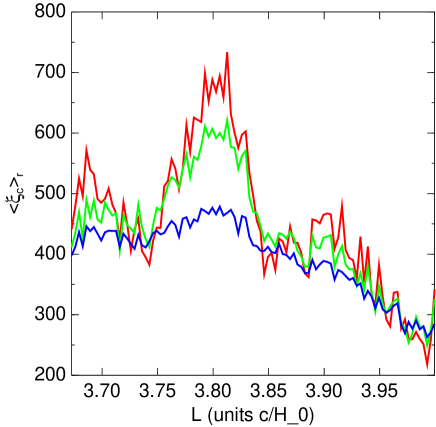
The coordinates of the Aurich (2008) $T^{3}$ solution are given in Table 1. We check the cross-correlation $\xi_{\mathrm{C}}$ (Roukema et al. 2008b) on the 9-year WMAP internal linear combination (ILC) map, using the corresponding KQ85 galactic contamination mask (Bennett et al. 2013), and show the dependence of the sub-gigaparsec-scale mean cross-correlation

$$\left<\xi_{\mathrm{C}}\right>_{r}(L):=\frac{1}{r}\int_{0}^{r}\xi_{\mathrm{C}}(r^{\prime},L)\mathrm{d}r^{\prime}$$ (1)

in Fig. 1. The cross-correlation $\xi_{\mathrm{C}}$ is a two-point correlation function that at small scales correlates pairs of points that are observed to be separated by large distances but according to the hypothesised 3-manifold are also separated by a small distance. The cross-correlation should be low if the hypothesis is wrong (Fig. 2 Roukema et al. 2008b) and high if the hypothesis is correct (Fig. 3 Roukema et al. 2008b). The strongest cross-correlation in Fig. 1 occurs for $L^{T^{3}}\approx 3.80\pm 0.05$ (in units of $c/H_{0}$), where the uncertainty is the half-width of the maximum at its base. The Aurich (2008) uncertainties are estimated from the pseudo-probability function used in the Monte Carlo Markov Chain search for an optimal solution. Since the pseudo-probability estimator is not a true probability, other methods are needed to estimate a realistic uncertainty. Figure 9 of Aurich (2008), showing the estimates in different foreground-subtracted single waveband WMAP maps, suggests $\sigma(L^{T^{3}})\approx 0.02$, combining random and some systematic sources of error (ILC versus single band maps). The shift by $0.05(c/H_{0})$ between Aurich (2008)’s estimate of $L^{T^{3}}$ for WMAP5 data and that shown in Fig. 1 suggests that inclusion of systematic error would give $\sigma(L^{T^{3}})\,\lower 2.58334pt\hbox{$\buildrel>\over{\sim}$}\,0.05$, i.e. 150$h^{-1}$ Mpc, rather than $\sigma(L^{T^{3}})=0.02$. The angular uncertainty given by Aurich (2008), $2^{\circ}$, is similar to that of the Poincaré dodecahedral space solution found earlier with the optimal cross-correlation method (Roukema et al. 2008b; Roukema et al. 2008a), i.e. a few hundred comoving $h^{-1}$ Mpc in a tangential direction at a radial distance of 5 to 10 $h^{-1}$ Gpc.

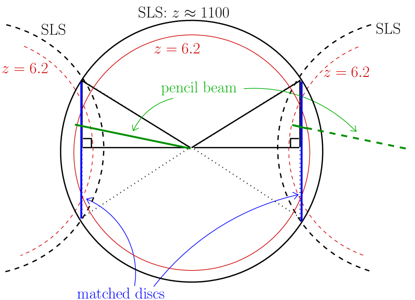
Leaving aside these uncertainties for the moment, the observationally most dramatic element of this $T^{3}$ solution is revealed by considering the redshift of an object topologically lensed in opposite directions along a fundamental axis. Aurich (2008) shows this in his Fig. 10 and briefly discusses it. Here, we use the principle of matched discs (Roukema & Kazimierczak 2011), shown with some extra detail in Fig. 2, and Table 2, listing the redshifts at the centres of a pair of matched discs and at circles increasing radially outwards to form the pair of matched discs. The fractional sky coverage $\omega/(4\pi)=12\pi(1-\cos\beta)/(4\pi)$, for discs of angular radius $\beta$, is also shown.

Given the rapidly increasing numbers of observed objects in the $5\,\lower 2.58334pt\hbox{$\buildrel<\over{\sim}$}\,z\,\lower 2.58334pt\hbox{$\buildrel<\over{\sim}$}\,6$ range, the beginning of detections around $6\,\lower 2.58334pt\hbox{$\buildrel<\over{\sim}$}\,z\,\lower 2.58334pt\hbox{$\buildrel<\over{\sim}$}\,8$, and the large fractional covering of the sky by the matched discs, it is obvious that independently of the few hundred $h^{-1}$ Mpc uncertainties in the $T^{3}$ solution, the observational data to reject or confirm the solution to very high statistical significance are going to become available over the next decade or two. The absence of topologically lensed images of quasars can be interpreted as a problem of their short lifetimes and highly anisotropic nature (beamed jets), but the absence of topologically lensed images of early forming galaxies would be much more difficult to explain.

Let us return to the uncertainty in the $T^{3}$ solution parameters. Pencil beam observations (“deep fields”) that probe to $z\sim 6$ have typical widths of at most a few arcminutes, i.e. a few $h^{-1}$ Mpc in comoving thickness at these redshifts. Thus, an accuracy of a few hundred $h^{-1}$ Mpc suggests that deep fields of a few degrees in size—pointed in the appropriate directions—will most likely be needed. The fourth row of entries in Table 2 shows the redshifts at the $\beta=10^{\circ}$ radius circle for $L^{T^{3}}=4.0$, i.e. $4\sigma$ greater than the WMAP9-ILC estimate shown in Fig. 1 if $\sigma$ is defined as the absolute difference between the Aurich (2008) WMAP5 estimate and the WMAP9-ILC estimate made here. Thus, for surveys limited to, e.g. $z<6.2$, observations closer to the face centres would better test the solution.

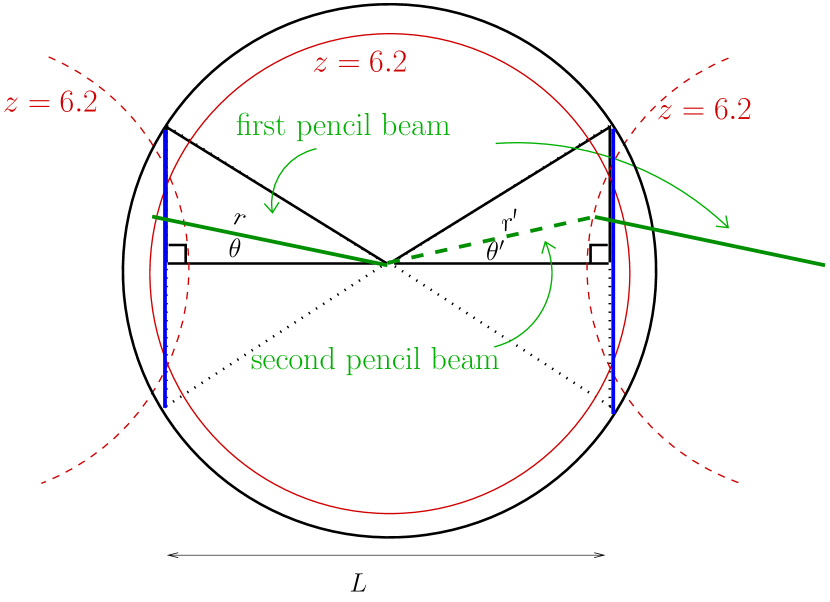
Figure 2 also shows a pair of not-quite-matched beams. These are not truly matched, since they exactly match only where they intersect the matched discs. The topologically matched parts of the two beams to the left (in Fig. 2) of their respective discs occur in the left-hand copy of the beam at slightly higher redshifts and in the right-hand copy at slightly lower redshifts, with respect to the redshift of the intersections with the matched discs. Since realistic surveys usually have wide redshift distributions, there is a fair chance of covering the topologically lensed region. However, this requires that the survey of the right-hand copy (in this figure) of the beam be wide enough in solid angle to cover the projection of the “beam” onto the sky, since the right-hand copy is not a beam from the observer’s point of view. For a small angular distance of the left-hand copy of the beam from the matched disc centre, the projected solid angle of a small portion of the right-hand copy will not be too large. Thus, for a small angular offset from the matched disc centres (axes of the fundamental domain), “not-quite-matched beams” can potentially test topological lensing hypotheses. The relation between an object near a matched disc centre and its topological image is illustrated (for the $T^{3}$ case) in Fig. 3, giving

$$\theta^{\prime} = \mathrm{atan}\left(\frac{r\sin\theta}{L-r\cos\theta}\right)$$

$$r^{\prime} = \frac{r\sin\theta}{\sin\theta^{\prime}}.$$ (2)

While matched discs and not-quite-matched beams indicate the parts of the sky that should be observed, detecting a significant statistical signal and generating a list of candidate pairs of topologically lensed objects requires a sensitive statistical method. This is presented below in Sect. 2.4. However, first we need to consider existing, planned and possible surveys in the three-dimensional regions of interest.

Table 3: Number of astrophysical objects with $5\leq z\leq 6.2$ and within 10^∘ of the Aurich (2008) $T^{3}$ solution fundamental axes (numbered as in Table 1) listed in NED^a as of 28 Oct 2012.

$$\begin{array}[]{c rrr rrr}\hline\cr\hline\cr i&1&2&3&4&5&6\\ \hline\cr\mbox{NED count}&44&0&0&9&1&0\\ \hline\cr\end{array}$$

^aNASA/IPAC Extragalactic Database, (http://ned.ipac.caltech.edu)

Table 4: Some well-known deep fields and their angular distance $\theta_{i}$ from the nearest $T^{3}$ axis (listed if $\theta\leq 20^{\circ}$).

$$\begin{array}[]{r rrrrr}\hline\cr\hline\cr\rule[-4.73611pt]{0.0pt}{13.77771pt}\mathrm{name}&l&b&\mathrm{min}_{i=1}^{6}(\theta_{i})&l_{T^{3}}&b_{T^{3}}\\ \mathrm{unit}&{}^{\circ}&{}^{\circ}&{}^{\circ}&{}^{\circ}&{}^{\circ}\\ \hline\cr\rule{0.0pt}{10.76385pt}\mathrm{VVDS}~{}\mbox{0226$-$04}^{a}\ignorespaces&172.&-58.&20.&186.&-77.\\ \mathrm{CDFS}^{b}\ignorespaces&224.&-54.&26.\\ \mbox{HDF-S}^{c}\ignorespaces&328.&-49.&52.\\ \mathrm{VVDS}~{}\mbox{2217+00}^{a}\ignorespaces&63.&-44.&50.\\ \mathrm{VVDS}~{}\mbox{1003+01}^{a}\ignorespaces&238.&43.&46.\\ \mathrm{HDF}^{d}\ignorespaces&126.&55.&43.\\ \mathrm{AEGIS}^{e}\ignorespaces&97.&60.&33.\\ \mathrm{VVDS}~{}\mbox{1400+05}^{f}\ignorespaces&343.&63.&16.&6.&77.\\ \mathrm{SDF}^{g}\ignorespaces&38.&83.&8.&6.&77.\\ \hline\cr\end{array}$$

^aVIRMOS Very Deep Survey (Le Fèvre et al. 2003)
^bChandra Deep Field South (Giacconi et al. 2001;
http://www.eso.org/~vmainier/cdfs_pub/CDFSfield.html)
^cHubble Deep Field-South “WPFC2 (apex) pointing” (Williams et al. 2000;
http://www.stsci.edu/ftp/science/hdfsouth/coordinatesS.html)
^dHubble Deep Field (Williams et al. 1996)
^eAll-Wavelength Extended Groth Strip International Survey (Davis et al. 2007)
^fIovino et al. (2005)
^gSubaru Deep Field (Maihara et al. 2001)

Table 5: Known objects^a near the northern galactic matched disc at sky position $(l_{1},b_{1})$ and redshift $z_{1}$ and their predicted most likely southern galactic positions $(l_{2},b_{2})$ and redshifts $z_{2}$, and redshift and cosmological time differences $\Delta z:=z_{1}-z_{2}$ and $\Delta t:=t_{2}-t_{1}$ (in $h^{-1}$ Myr), respectively, assuming metric parameters $\Omega_{\mathrm{m}}=0.28,\Omega_{\mathrm{r}}=1.65\times 10^{-4}\Omega_{\mathrm{m}},\Omega_{\Lambda}=1-\Omega_{\mathrm{m}}-\Omega_{\mathrm{r}}$ and the $T^{3}$ fundamental axis $(l=6^{\circ},b=+77^{\circ})$ of length $L=11.4{\mbox{$h^{-1}$ Gpc}}$.

$$\begin{array}[]{l ccc ccc rr}\hline\cr\hline\cr\rule{0.0pt}{10.76385pt}\mbox{name}&l_{1}&b_{1}&l_{2}&b_{2}&z_{1}&z_{2}&\Delta z&\Delta t\\ \hline\cr\rule{0.0pt}{10.76385pt}\mbox{{[SKD2006]~{}017721}}&35.597&82.506&174.850&-70.004&5.724&5.281&0.443&75.6\\ \mbox{{[SKD2006]~{}036334}}&36.053&82.455&174.632&-70.020&5.705&5.300&0.405&69.2\\ \mbox{{[SKD2006]~{}034503}}&36.000&82.515&174.771&-69.984&5.698&5.308&0.390&66.6\\ \mbox{SDF~{}J132519.4+271829}&36.238&82.470&174.368&-69.758&6.000&5.058&0.942&160.2\\ \mbox{[SKD2006]~{}018699}&35.605&82.619&175.130&-69.980&5.645&5.356&0.289&49.4\\ \mbox{[SKD2006]~{}020087}&35.642&82.613&175.045&-69.917&5.724&5.286&0.438&74.8\\ \mbox{[SKD2006]~{}031858}&35.934&82.554&174.870&-69.965&5.692&5.314&0.378&64.5\\ \mbox{SDSS~{}J134040.24+281328.1}^{b}\ignorespaces&41.523&79.054&165.545&-71.950&5.338&5.654&-0.315&-53.9\\ \mbox{[SKD2006]~{}020495}&35.635&82.719&175.272&-69.858&5.697&5.314&0.383&65.4\\ \mbox{SDF~{}J132426.5+271600}&35.900&82.666&174.836&-69.609&6.030&5.039&0.991&168.2\\ \mbox{[SKD2006]~{}023759}&35.721&82.737&175.288&-69.846&5.687&5.324&0.363&61.9\\ \mbox{[SKD2006]~{}031765}&35.920&82.705&175.167&-69.852&5.691&5.321&0.370&63.1\\ \mbox{[SKD2006]~{}073078}&37.030&82.493&174.428&-69.913&5.700&5.314&0.386&65.8\\ \mbox{[SKD2006]~{}027787}&35.814&82.765&175.300&-69.801&5.707&5.308&0.399&68.0\\ \mbox{[SKD2006]~{}046904}&36.307&82.703&175.075&-69.843&5.665&5.347&0.318&54.2\\ \mbox{[SKD2006]~{}042576}&36.182&82.745&175.175&-69.806&5.684&5.331&0.353&60.2\\ \mbox{[SKD2006]~{}039849}&36.112&82.767&175.232&-69.788&5.692&5.324&0.368&62.7\\ \mbox{[SKD2006]~{}050215}&36.394&82.720&175.070&-69.809&5.682&5.333&0.349&59.4\\ \mbox{SDF~{}J132501.3+272628}&37.258&82.538&174.767&-70.166&5.337&5.666&-0.329&-56.1\\ \mbox{SDF~{}J132442.5+272423}&36.992&82.607&174.394&-69.554&6.040&5.038&1.002&169.8\\ \mbox{SDF~{}J132345.6+271701}&36.019&82.817&175.043&-69.415&6.110&4.986&1.124&190.4\\ \mbox{[SKD2006]~{}061418}&36.716&82.675&174.839&-69.763&5.748&5.276&0.472&80.3\\ \mbox{[SKD2006]~{}048328}&36.338&82.782&175.196&-69.758&5.693&5.325&0.368&62.6\\ \mbox{[SKD2006]~{}093966}&37.603&82.523&174.308&-69.824&5.721&5.302&0.419&71.4\\ \mbox{[SKD2006]~{}070600}&36.978&82.784&175.054&-69.738&5.654&5.366&0.288&49.0\\ \mbox{[SKD2006]~{}096007}&37.679&82.641&174.544&-69.752&5.696&5.329&0.367&62.5\\ \mbox{[SKD2006]~{}124783}&38.436&82.458&173.942&-69.801&5.720&5.308&0.412&70.1\\ \mbox{[SKD2006]~{}095588}&37.672&82.650&174.530&-69.710&5.738&5.292&0.446&75.8\\ \mbox{[SKD2006]~{}084305}&37.352&82.740&174.832&-69.706&5.695&5.331&0.364&62.0\\ \mbox{[SKD2006]~{}124530}&38.442&82.515&174.085&-69.784&5.689&5.337&0.352&59.8\\ \mbox{[SKD2006]~{}084720}&37.374&82.768&174.891&-69.695&5.682&5.343&0.339&57.6\\ \mbox{[SKD2006]~{}132343}&38.639&82.481&173.954&-69.785&5.697&5.331&0.366&62.3\\ \mbox{[SKD2006]~{}121315}&38.376&82.624&174.302&-69.688&5.716&5.317&0.399&67.8\\ \mbox{[SKD2006]~{}113271}&38.176&82.675&174.464&-69.673&5.710&5.322&0.388&65.9\\ \mbox{[SKD2006]~{}126848}&38.522&82.593&174.197&-69.697&5.718&5.315&0.403&68.4\\ \mbox{[SKD2006]~{}108164}&38.033&82.762&174.709&-69.653&5.672&5.358&0.314&53.4\\ \mbox{[SKD2006]~{}152586}&39.251&82.713&174.280&-69.578&5.681&5.359&0.322&54.7\\ \mbox{[SKD2006]~{}154296}&39.280&82.709&174.235&-69.550&5.715&5.329&0.386&65.5\\ \mbox{[SKD2006]~{}166310}&39.595&82.696&174.140&-69.547&5.698&5.346&0.352&59.6\\ \mbox{[SKD2006]~{}158036}&39.404&82.755&174.329&-69.540&5.676&5.366&0.310&52.5\\ \mbox{[SKD2006]~{}168127}&39.668&82.757&174.268&-69.518&5.674&5.370&0.304&51.4\\ \mbox{[SKD2006]~{}163079}&39.556&82.785&174.353&-69.505&5.676&5.368&0.308&52.1\\ \mbox{SDSS~{}J133412.56+122020.7}^{b}\ignorespaces&339.134&72.136&223.205&-77.385&5.134&5.962&-0.828&-139.6\\ \mbox{SDSS~{}J140940.72+274507.1}^{c}\ignorespaces&39.513&72.652&146.699&-75.339&5.359&5.819&-0.460&-76.1\\ \hline\cr\end{array}$$

^aThe objects are galaxies except where otherwise indicated. ^bQSO. ^cObject type uncertain.

2.2 Observational catalogues

2.2.1 Existing observations

Table 3 shows that almost all of the $z\sim 6$ objects that are so far known near the $T^{3}$ axes are those near the high galactic latitude, northern fundamental direction 1, although a few are also known near the corresponding southern fundamental direction 4. Most of the northern objects are from the Subaru Deep Field observed with the Cooled Infrared Spectrograph and Camera for [the] OH airglow suppressor (CISCO, Motohara et al. 2002) on the 8.2 m Subaru telescope (Maihara et al. 2001; Shimasaku et al. 2006), listed along with some of the other well-known deep fields in Table 4. The galactic coordinates and redshifts of the northern objects are listed as part of Table 5.

2.2.2 Planned and possible observations

First let us consider high-redshift quasars. The VISTA/VIKING 4-m class telescope project should discover quasars at $z\sim 7$ over about 1500 deg² centred on the northern and southern Galactic poles (Findlay et al. 2011). Although Table 2 here and the expected completeness levels shown in Fig. 13 of Findlay et al. (2011) indicate that coverage of the desired regions is possible (depending on the value of $\Omega_{\mathrm{m}}$), only about 8 quasars are expected in the whole survey (Sect. 4.1, Findlay et al. 2011), clearly too low to obtain significant evidence either for or against the $T^{3}$ candidate.

Polsterer et al. (2012) find 22,992 photometric quasar candidates with $5.5<z<6.2$ and an estimated error of $\sigma(\Delta z)=0.087$, expecting about half the candidates to be true quasars. However, the solid angle from which the quasars are selected is about $2\pi$, giving a candidate surface density of about 1/deg² and an expected spectroscopic number density of about 0.5/deg² if a complete spectroscopic followup were to be performed. This is about 100 times higher than for the VISTA/VIKING survey (as presently designed), but still somewhat low. While quasars dominated high-redshift records for the decades when $z>1$ was considered a high redshift for a spectroscopically confirmed extragalactic object, this seems less likely at $z\sim 6$. For a given apparent magnitude limit, it is clear that LBG and LAE catalogues are present in much high number densities at $z\sim 6$.

Plans for LBG and LAE searches typically focus on the existing “deep fields”, with the aims of achieving wide coverage across the electromagnetic spectrum. Several of these fields and their angular distances $\theta_{i}$ from the closest $T^{3}$ axes are given in Table 4, indicating which fields would be the most useful for testing the $T^{3}$ candidate via LBG and LAE searches. Comparison with Table 2 indicates that for $5\,\lower 2.58334pt\hbox{$\buildrel<\over{\sim}$}\,z\,\lower 2.58334pt\hbox{$\buildrel<\over{\sim}$}\,7$ searches, the Subaru Deep Field and its corresponding northern region is optimal, while for $5.5\,\lower 2.58334pt\hbox{$\buildrel<\over{\sim}$}\,8$ searches, the Virmos Very Deep Survey fields 0226$-$04 and 1400+05 and their northern and southern, respectively, counterparts would be worth observing.

The EUCLID mission planned for launch in 2019 has a deep survey (Sect. 1.3, Refregier et al. 2010), the EUCLID optical and NIR Deep Imaging Survey, planned over 40 deg². This should obtain “thousands” of likely LBG’s and LAE’s with $z>6$ based on photometric redshifts (Sect. 14.2, Refregier et al. 2010), i.e., $\,\lower 2.58334pt\hbox{$\buildrel>\over{\sim}$}\,50$/deg². If a few objects had quadruple multiplicities that made them very likely topological lensing candidates, then optical/near-infrared spectroscopic followup with an instrument such as X-Shooter (300 nm $\,\lower 2.58334pt\hbox{$\buildrel<\over{\sim}$}\,\lambda\,\lower 2.58334pt\hbox{$\buildrel<\over{\sim}$}\,$ 2400 nm, Vernet et al. 2011) on the Very Large Telescope (VLT) on the southern objects and corresponding spectra of the northern objects with the Keck or Subaru telescopes should obtain enough rest-frame spectral energy distribution information to check whether the would-be topologically lensed pairs of objects resembled each other more than would be expected for arbitrary pairs of objects at similar redshifts. The Multi Unit Spectroscopic Explorer (MUSE) on the VLT, which should be well-tested by the time that the EUCLID data are available, would be useful for secondary followup to study the spatial environments of the candidate lensed objects, especially when the cosmological time difference between the members of a pair is small compared to a typical galaxy dynamical time scale.

Thus, we should simulate several square degrees of observations with parameters consistent with those estimated for EUCLID. In particular, it would be interesting to see if a statistical signal could be obtained from photometric redshifts alone, prior to spending high amounts of exposure time on highly sought after telescope/instrument combinations.

The Ultra-Deep Survey of the James Webb Space Telescope (JWST) should detect galaxies at $z\,\lower 2.58334pt\hbox{$\buildrel>\over{\sim}$}\,6$, but over only about 10 arcmin² (Sect. 2, Table II, Gardner et al. 2006). The JWST’s planned Deep Wide Survey should find galaxies over $1\,\lower 2.58334pt\hbox{$\buildrel<\over{\sim}$}\,z\,\lower 2.58334pt\hbox{$\buildrel<\over{\sim}$}\,6$ over a larger solid angle, 100 arcmin² (Sect. 3.6, Table III, Gardner et al. 2006). For an initial uncertainty of about two degrees in the $T^{3}$ axes, these surveys are clearly too narrow.

2.3 Simulations

Simulating searches for matched quadruples requires comparison of observations in a $T^{3}$ model to those in an $\mathbb{R}^{3}$ model. The existing Subaru Deep Field observations are used to provide an observationally based simulation of both sorts, in which the southern field is generated for the $T^{3}$ model by applying the Aurich (2008) $T^{3}$ holonomy (Table 1) to the Subaru galaxies, and simulated independently of real observations in the case of the $\mathbb{R}^{3}$ model. For a hypothetical observational program aimed at the centres of both the 1–4 axis expected matched discs, fully simulated data are needed in both cases.

The spatial two-point auto-correlation function $\xi(r)$ could, in principle, lead to excess non-topological chance isometries if the tolerances for requiring isometry are not tight enough. For the low number densities of objects expected, the effect is unlikely to be strong. Half of a large number of points are first generated uniformly within a redshift shell defined by the required redshift limits. Each further point is chosen by randomly choosing an existing point, and placing the new point in a 3-Euclidean direction chosen uniformly from $4\pi$ ster at a comoving distance chosen with the probability $P(r,\mathrm{d}r)\propto 1+\xi(r)$, where

$$\xi(r)=\left\{\begin{array}[]{l l}\left(\frac{r_{0}}{r_{\min}}\right)^{\gamma},&r\leq r_{\min}\\ \left(\frac{r_{0}}{r}\right)^{\gamma},&r_{\min}\leq r<r_{\max}\\ 0,&r\geq r_{\max},\end{array}\right.$$ (3)

for a correlation length $r_{0}$ and power law index $\gamma$, and numerical cutoffs $r_{\min}$ and $r_{\max}$. Points that do not fall in the redshift shell are ignored, and new points are generated in the same way until the required number fill the shell. Numerical measurement of the resulting simulated distributions shows that in practice, this simulates a stronger correlation than that required. Thus, the chance of non-topological isometries is overestimated, i.e. our results are conservative: real observations are less likely to give a false positive detection. Moreover, in order to err on the side of possibly underestimating the numbers of matching quadruples in the multiply connected case, the correlation function is not used when simulating this case; uniform distributions are drawn from instead. Again, this is conservative: we slightly underestimate the statistical significance of the method (Sect. 2.5).

Peculiar velocities and the uncertainties in redshift estimation need to be simulated (Roukema 1996). Photometric redshift errors are those of most interest here: are they small enough to significantly discriminate between signal and noise? These errors are all simulated radially using a peculiar rapidity ${\phi}_{\mathrm{pec}}$ selected from a Gaussian distribution of mean zero and standard deviation $\;\mathrm{atanh}(\sigma({\beta}_{\mathrm{pec}}))\;$ for a single input parameter, the peculiar velocity standard deviation $\sigma({\beta}_{\mathrm{pec}})$, and using Eq. (15), where ${\beta}_{\mathrm{pec}}=\tanh{\phi}_{\mathrm{pec}}$ and ${z}_{\mathrm{pec}}=[(1+{\beta}_{\mathrm{pec}})/(1-{\beta}_{\mathrm{pec}})]^{1/2}-1.$ Use of rapidities rather than velocities avoids the unphysical case of $|{\beta}_{\mathrm{pec}}|\geq 1$ for simulating photometric redshifts with high $\sigma({\beta}_{\mathrm{pec}})$.

Before applying the holonomies in a given simulation, random Gaussian errors are added to the $T^{3}$ axis parameters given in Table 1. “Observations” of the simulated catalogues are carried out in galactic coordinate limited regions in the expected position(s).

2.4 The successive filter method for type I pairs

Lehoucq et al. (1999) introduced the terminology of type II pairs and type I pairs (or $n$-tuples), that had been introduced earlier by Lehoucq et al. (1996) and Roukema (1996), respectively. Type I pairs or $n$-tuples can be thought of as the matching between a local region of objects and its distant copy. Since a holonomy for an FLRW multiply connected model is an isometry, the distances among the members within the “original” region should correspond to the distances among the members of the copy of that region. A Type II pair—in a space such as $T^{3}$—corresponds to an object and its copy. In $T^{3}$, this separation is a vector in the covering space $\mathbb{R}^{3}$. Difficulties in finding statistically significant numbers of either type of pair given realistic observational parameters and noise led to a new way of collecting type I pairs (Uzan et al. 1999) and a successive filter method (Marecki et al. 2005). Fujii & Yoshii (2011) presented a variation on the successive filter method, along with an analysis step that is roughly equivalent to collecting together $n$-tuples of mixed type for all $n\geq 4$ or to the Marecki et al. (2005) bunches of pairs filter (Sect.  3.2.5, Fujii & Yoshii 2011). The latter step, made possible by the successive filters, significantly reduces the combinatorial problem presented in Roukema (1996). A catalogue containing two distant regions, each with $N$ objects, might contain just one pair of matched $n$-tuples across the two regions, but searching for all $({}^{N}C_{n})^{2}$ combinations of objects with $N=100$ and $n=7$ would require $10^{20}$ comparisons of 7-tuples. Fujii & Yoshii (2011) use toy simulations to show that a very small number of matched $n$-tuples can be detected by the full method of successive filtering and collecting.

The successive filter method implemented here tests four simulated (and/or real) galaxies at $(x,y,z)(i),$ $(x,y,z)(j),$ $(x,y,z)(k),$ and $(x,y,z)(l)$ via the following filters in the following order, where $(i,j,k,l)$ is an ordered choice of unequal indices in the list of galaxies. A crossed quadruple parameter $\chi(\mathbf{q})\in\mathbb{Z}_{2}$ is defined for a given ordered quadruple $\mathbf{q}=(i,j,k,l)$ in order to relate the lifetime and bunches of pairs (BoP) filters (Marecki et al. 2005). This algorithm allows the pair separations $d$, where $d(.,.)$ is the comoving distance between two arbitrary points in the covering space $\mathbb{R}^{3}$, the (signed) $x,y,z$ component separations of each pair, to be calculated first, and the loop for finding quadruples to be performed over pairs of pairs. Arithmetically, the change from subtraction to addition of pair separations in the BoP filter is equivalent to swapping an $((i,j),(k,l))$ pair of ordered pairs to $((i,k),(j,l))$. The filters are:

• type I pair filter:

  $$|d(i,j)-d(k,l)|<\epsilon,$$ (4)

• lifetime filter:

  $$|t_{i}-t_{k}|<\Delta t\;\mathrm{and}\;|t_{j}-t_{l}|<\Delta t \Rightarrow \chi((i,j,k,l))=0,\;\mathrm{or}$$

  $$|t_{i}-t_{l}|<\Delta t\;\mathrm{and}\;|t_{j}-t_{k}|<\Delta t \Rightarrow \chi((i,j,k,l))=1,\;\mathrm{or}$$

  otherwise: $$\mbox{filter fails,}\;\nexists\chi$$ (5)

• BoP filter:

  $$\Big{(}\chi((i,j,k,l))=0 \mathrm{and} \big{|}[x(i)-x(j)]-[x(k)-x(l)]\big{|}<\epsilon_{\mathrm{BoP}}$$

  $$\mathrm{and} \big{|}[y(i)-y(j)]-[y(k)-y(l)]\big{|}<\epsilon_{\mathrm{BoP}}$$

  $$\mathrm{and} \big{|}[z(i)-z(j)]-[z(k)-z(l)]\big{|}<\epsilon_{\mathrm{BoP}}\Big{)}$$

  $$\mathrm{or}$$

  $$\Big{(}\chi((i,j,k,l))=1 \mathrm{and} \big{|}[x(i)-x(j)]+[x(k)-x(l)]\big{|}<\epsilon_{\mathrm{BoP}}$$

  $$\mathrm{and} \big{|}[y(i)-y(j)]+[y(k)-y(l)]\big{|}<\epsilon_{\mathrm{BoP}}$$

  $$\mathrm{and} \big{|}[z(i)-z(j)]+[z(k)-z(l)]\big{|}<\epsilon_{\mathrm{BoP}}\Big{)}.$$

Substituting a difference test for the BoP filter above, i.e. $|d(i,j)-d(k,l)|<\epsilon_{\mathrm{BoP}}$ and $|d(i,k)-d(j,l)|<\epsilon_{\mathrm{BoP}}$ for the uncrossed and crossed pairs of pairs, respectively, would allow non-planar quadrilaterals (fold a rectangular sheet of paper along its diagonal to see this), whereas only a parallelogram can represent a $T^{3}$ topological quadruple.

A list of quadruples (pairs of pairs, each associated with a crossed quadruple parameter $\chi$) that satisfy all three successive filters is obtained. An arbitrary galaxy $i$ is a member of $s_{i}\geq 0$ quadruples. The frequency of $s$ in a given simulated set of galaxies is $f(s)$, i.e.

$$f(s):=|\{i:s_{i}=s\}|.$$ (7)

If a topological lensing signal is present, there should be a high number of galaxies which are a member of many quadruples, $f(s)$ should be high for high $s$. This is a critical step in the successive filter method, introduced in Sect. 3.2.5 of Fujii & Yoshii (2011): for $s\gg 1$, the statistic $f(s)$ should be significantly higher in a catalogue containing topological lensing than in a simply connected catalogue.

2.5 Statistical significance

For an arbitrary realisation, let us define the cumulative number of galaxies that are each members of many quadruples

$$F(s^{*}):=\sum_{s>s^{*}}f(s),$$ (8)

for some quadruplet membership number $s^{*}>0$, which formalises the word “many” in “many quadruples”. Thus, for a fixed value $s^{*}$, $F$ is a random variable which we model numerically. To estimate what observational strategy is required to have a low chance of a false negative inference from the data, i.e. to find $\beta$, the expected probability of falsely excluding the $T^{3}$ hypothesis, suppose that the observational result gives $F=i$ for some non-negative integer $i$. Then the probability of falsely excluding the Aurich (2008) $T^{3}$ hypothesis is the cumulative probability $P(F\leq i|T^{3})$, which can be estimated numerically by finding the fraction of $T^{3}$ simulations for which $F\leq i$.

Since we don’t yet know the results of the observations, we have to weight this over $p(F=i|\mathbb{R}^{3})$, the probability density function of $i$ for the simply connected case. Thus, the expectation value of the probability of falsely rejecting the hypothesis $P(F\leq i|T^{3})$ (which itself is a random variable) is

$$p_{0} = \mathrm{E}[P(F\leq i|T^{3})]$$ (9)

$$= \sum_{i=0}^{\infty}\left(p(F=i|\mathbb{R}^{3})\;P(F\leq i|T^{3})\right).$$

Similarly, to estimate what observational strategy is required to have a low chance of a false positive inference from the data, the expected probability of falsely supporting the $T^{3}$ hypothesis can be written

$$\sum_{i=0}^{\infty}\left(p(F=i|T^{3})\;P(F\geq i|\mathbb{R}^{3})\right).$$ (10)

$$= \sum_{i=0}^{\infty}\left[p(F=i|T^{3})\;\left(\sum_{j=i}^{\infty}p(F=j|\mathbb{R}^{3})\right)\right].$$

$$= \sum_{i=0}^{\infty}\sum_{j=i}^{\infty}\left[p(F=i|T^{3})\;\left(p(F=j|\mathbb{R}^{3})\right)\right].$$

$$= \sum_{j=0}^{\infty}\sum_{i=0}^{j}\left[p(F=i|T^{3})\;\left(p(F=j|\mathbb{R}^{3})\right)\right].$$

$$= p_{0},$$

i.e. the two expectation values are equal.

Figure 4: Quadruple frequencies $N(s)$ obtained by the successive filter method (Sect. 2.4) applied to sets of objects in the multiply connected (dark curve, red online) and simply connected (pale curve, green online) cases, using the known, northern galactic objects in the SDF (second, third and sixth columns of Table 5). The southern object set is calculated using the Aurich (2008) $T^{3}$ model in the multiply connected case, and simulated with an input auto-correlation function $r_{0}=10.0{\mbox{$h^{-1}$ Mpc}},\gamma=1.8,r_{\min}=1.0{\mbox{$h^{-1}$ Mpc}},r_{\max}=100.0{\mbox{$h^{-1}$ Mpc}}$ in the simply connected case. The southern field is “observed” over 1 deg² at the expected position in both cases. Top: Successive filter parameters (Sect. 2.4) are $\epsilon=1.0{\mbox{$h^{-1}$ Mpc}},\Delta t=0.01{\mbox{$h^{-1}$ Gyr}},\epsilon_{\mathrm{BoP}}=1.0{\mbox{$h^{-1}$ Mpc}}$. Bottom: Same, except that $\Delta t=1{\mbox{$h^{-1}$ Gyr}}$.

Figure 5: Quadruple frequencies $N(s)$, as for Fig. 4, but a realisation of Gaussian uncertainties in the $T^{3}$ parameters is applied, destroying the topological signal, since none of the implied topological images fall in the southern field in this realisation.

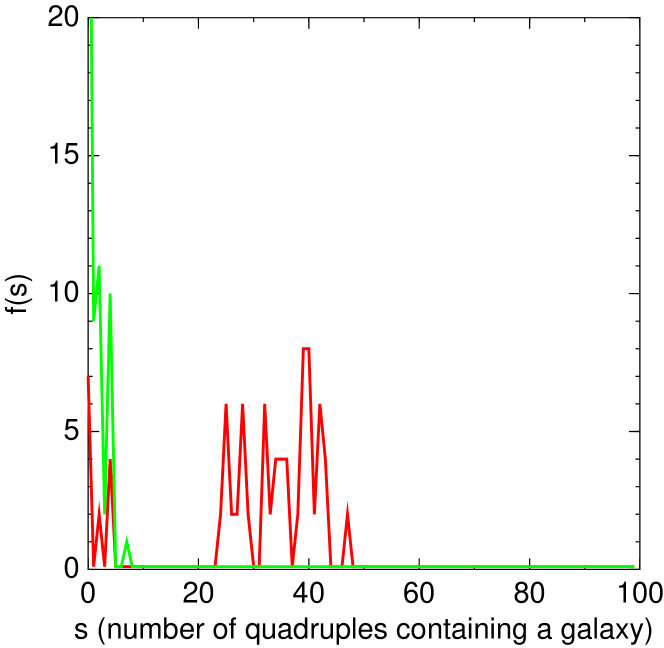
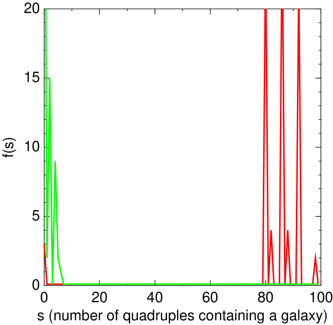
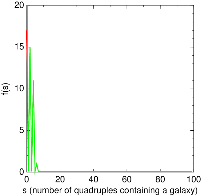
For a given simulation parameter set, a set of simulations is analysed for each $s^{*}\in\{1,\dots,10\},$ a range that is found below (Sect. 3) by inspection of $N(s)$ versus $s$ histograms for typical realisations. The minimum

$$p_{1}:=\min_{s^{*}}p_{0}$$ (11)

determines the $s^{*}$ value for the optimal statistical test for the simulation parameter set, and the expectation value of the probability of falsely excluding the $T^{3}$ hypothesis or of falsely detecting evidence in favour of it.

3 Results

3.1 Existing observations

Table 5 lists observed objects and the implied positions where topologically lensed images should be observed if the $T^{3}$ hypothesis is correct, with zero uncertainty in the $T^{3}$ axis parameters given in Table 1). Figure 4 shows the application of the successive filters method under the assumption that a survey of one square degree in the redshift range $5<z<6.2$ is 100% complete in comparison to the surveys that found the high galactic latitude sample. The southern survey field is centred on the expected median celestial position of the implied objects (the fourth and fifth columns of Table 5). The topological signal is clearly very strong in Fig. 4, both for low $\Delta t=0.01$ $h^{-1}$ Gyr (top), in which case it is unlikely that stellar evolution would cause the earlier image of a galaxy to dim too much to be seen, and for high $\Delta t=1$ $h^{-1}$ Gyr, in which case dimming could weaken the test. The northern part of each catalogue analysed consists of the 44 known objects, there are 41 topologically implied objects within the southern field, and the simulated southern subset consists of 24 and 30 objects for $\Delta t=0.01$ $h^{-1}$ Gyr and 1 $h^{-1}$ Gyr), respectively.

Figure 6: As for Fig. 4, for fully simulated, multiply connected (dark, red online) and simply connected (pale, green online) catalogues, over northern and southern fields each of $\approx 64$ deg² centred at antipodal matched disc centres, with $4.3<z<6.6$, and successive filter parameters $\epsilon=2.0{\mbox{$h^{-1}$ Mpc}},\Delta t=1.0{\mbox{$h^{-1}$ Gyr}},\epsilon_{\mathrm{BoP}}=1{\mbox{$h^{-1}$ Mpc}}$, and (in the simply connected case) an input auto-correlation function $r_{0}=10.0{\mbox{$h^{-1}$ Mpc}},\gamma=1.8,r_{\min}=1.0{\mbox{$h^{-1}$ Mpc}},r_{\max}=100.0{\mbox{$h^{-1}$ Mpc}}$ [Eq. (3)]. A total of 300 simulated objects (north plus south) are present in each catalogue. Top: Spectroscopic redshifts. Bottom: Photometric redshifts with $\sigma({\beta}_{\mathrm{pec}})=0.005$, i.e. $\sigma(\Delta z)\approx 0.03$.

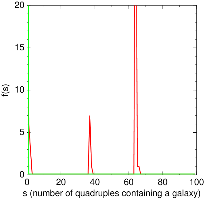
The uncertainty in the $T^{3}$ coordinates and fundamental length also need to be taken into account. An error of $2^{\circ}$ in the vector (in the flat comoving covering space) from the observer to an object at a matched disc centre implies an error of about twice the size in the observing angle of the implied image, because the diameter of the shell containing objects at the distance of the matched disc centres is twice the radius of the shell. Thus, as Fig. 5 shows, a typical realisation of a 1 deg² southern survey is very unlikely to detect any topological quadruples (satisfying the filter criteria). The total disappearance of the topological signal in this figure ($s=0$ for all objects, since there are no topological images lying within the southern field at all), making the $N(s)$ distribution even weaker than that of the simply connected data set, is an artefact of the method. We did not add any “background” simulated data around the northern galactic, observed SDF field, so the implied southern objects constitute a “survey” that contains less objects (zero) than the simulated southern survey (16 objects in Fig. 5). Thus, let us consider fully simulated surveys.

3.2 Planned or possible observations

Given the uncertainties in the $T^{3}$ solution discussed in Sect. 2.1 and listed in Table 1, let us consider a pair of northern and southern surveys centred on the matched disc centres for the same $T^{3}$ axis, each of 64 deg². As explained above, for a given known object, a two degree $T^{3}$ axis uncertainty yields an approximately four degree uncertainty for an observer placed halfway between the opposing images and searching for a topological image at the expected position. However, since we simulate both fields, other pairs of objects in the matched discs can be found, so $2^{\circ}$ should approximately correspond to a 68% chance (for one angle offset from a Gaussian distribution of width $2^{\circ}$) of finding matching pairs. Thus, 64 deg² should approximately correspond to a 2$\sigma$ (where $\sigma$ is one standard deviation) chance of finding topological pairs.

Figure 7: Expectation values $p_{1}$ of falsely rejecting (or falsely accepting) the $T^{3}$ hypothesis for optimal choices of $s^{*}$ [Eq. (11)], as a function of photometric redshift $\sigma(z_{\mathrm{phot}})$ [estimated as $(1+(z_{1}+z_{2})/2)\sigma({\beta}_{\mathrm{pec}})$, using $\sigma({\beta}_{\mathrm{pec}})\ll 1$ and Eq. (15), where $z_{1}<z<z_{2}$ is the redshift range], and the number of galaxies $N_{\mathrm{gal}}$ per combined (north plus south) catalogue. The lowest probabilities $p_{1}$ (highest significance) results are for low $\sigma(z_{\mathrm{phot}})$ and high $N_{\mathrm{gal}}$, at top-left in each of the panels. Top: $4.3<z<6.6$, solid angle per survey direction (south or north) $\omega\approx 100$ deg², $\Delta t=1$ $h^{-1}$ Gyr. The other parameters are identical to those for Fig. 6. Bottom: Same, except that $\Delta t=0.1$ $h^{-1}$ Gyr.

Figure 8: Expectation values $p_{1}$ of falsely rejecting (or falsely accepting) the $T^{3}$ hypothesis, as for Fig. 7, but for a thicker, wider survey, over $4<z<7$ and $\omega\approx 196$ deg². Top: $\Delta t=1$ $h^{-1}$ Gyr, Bottom: $\Delta t=0.1$ $h^{-1}$ Gyr,

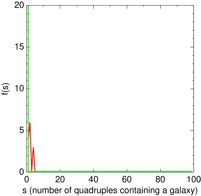
The uncertainty in $L^{T^{3}}$ gives a 1$\sigma$ uncertainty of about 150 $h^{-1}$ Mpc, i.e. a 2$\sigma$ uncertainty of 300 $h^{-1}$ Mpc. For a survey going from the matched disc centre to $\beta\approx 4^{\circ}$ away, Table 2 (for $\Omega_{\mathrm{m}}=0.28$) gives a typical redshift of $z\approx 5.38$, i.e. $5.706$ $h^{-1}$ Gpc in radial comoving distance from the observer. Inverting this, $5706\pm 300$ $h^{-1}$ Mpc gives $4.60\,\lower 2.58334pt\hbox{$\buildrel<\over{\sim}$}\,z\,\lower 2.58334pt\hbox{$\buildrel<\over{\sim}$}\,6.33$. We extend this a little to be conservative, and increase the filter criterion $\epsilon$ to 2 $h^{-1}$ Mpc. A typical realisation is shown in the top panel of Fig. 6. Clearly, a pair of surveys that are wide enough on the sky and in redshift coverage, finding 300 objects above an idealised, $z$-independent completeness limit, has a good chance of strongly rejecting or supporting the $T^{3}$ hypothesis.

Could photometric redshift estimates be sufficient? The lower panel of Fig. 6 shows the quadruple signal for a realisation with Gaussian peculiar velocity uncertainties simulated with $\sigma({\beta}_{\mathrm{pec}})=0.005$, i.e. a redshift uncertainty of $\sigma(\Delta z)\approx 0.03$. The signal is clearly much weaker, but (in this realisation) is still distinguishable from the $N(s)$ curve of the simply connected simulation.

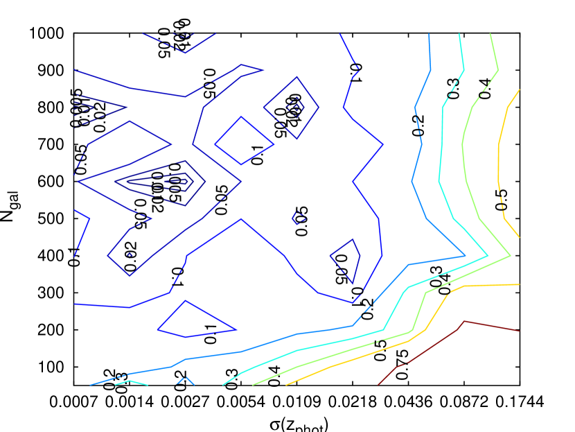
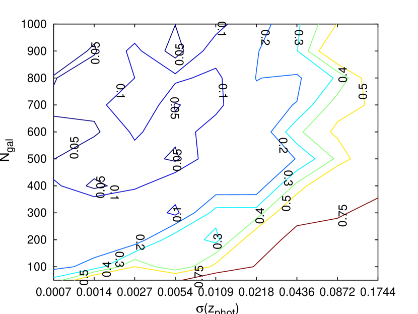
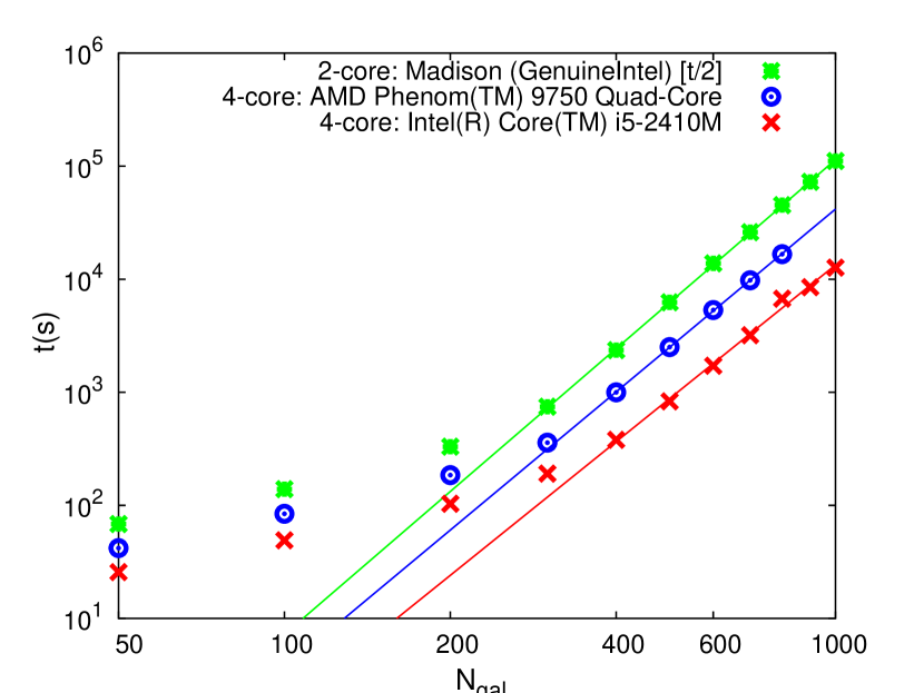
Figure 7 presents confidence levels, i.e. $p_{1}$, as defined in Eq. (11) in Sect. 2.5, from ensembles of realisations. Unsurprisingly, low $\sigma(\Delta z_{\mathrm{phot}})$ and high $N_{\mathrm{gal}}$ generally give the statistically most significant results. The dependence on these two parameters is not fully monotonic. This is understandable because for a fixed $\sigma(\Delta z_{\mathrm{phot}})$, higher $N_{\mathrm{gal}}$ not only increases the numbers of topological quadruples, it also increases the number density, so that the numbers of non-topological quadruples also increase, yielding some complexity in the dependence. There is some statistical noise in the contours. The total computing time for Fig. 7 on a single, recent 4-core processor would be from a few weeks to a few months (Appendix B). The actual calculations were performed using parallel computing resources on several different machines.

Figure 7 also shows that a typical photometric redshift error of $\sigma(\Delta z_{\mathrm{phot}})\,\lower 2.58334pt\hbox{$\buildrel<\over{\sim}$}\,0.01$ would enable rejection at $p_{1}\,\lower 2.58334pt\hbox{$\buildrel<\over{\sim}$}\,0.05$ (i.e. a $2\sigma$ rejection according to intuition for a Gaussian distribution), provided that $N_{\mathrm{gal}}\,\lower 2.58334pt\hbox{$\buildrel>\over{\sim}$}\,500$ in northern and southern surveys each over $\omega\approx 100$ deg². This is only a moderate confidence level for rejecting the hypothesis, but since $p_{1}$ also represents the expectation value of falsely accepting the hypothesis, it would be sufficient to provide a strong motivation for studying candidate topologically lensed galaxies further. A plot roughly similar to the lower panel of Fig. 6 would be obtained, enabling the particular galaxies most likely to be topologically lensed to be identified. The particular realisation in the lower panel of Fig. 6 shows about 10 galaxies that are each members of $s>1$ quadruples. This is a small enough number for spectroscopic followup to be relatively easy to obtain.

Comparison of the top and bottom panels in Fig. 7 illustrates the potential role of evolutionary effects. The lower panel limits type II pairs to those with $\Delta t=0.1$ $h^{-1}$ Gyr instead of $\Delta t=1$ $h^{-1}$ Gyr (upper panel). To attain moderate confidence, i.e. $p_{1}\,\lower 2.58334pt\hbox{$\buildrel<\over{\sim}$}\,0.05$, photometric redshift errors would need to be tightened to about $\sigma(\Delta z_{\mathrm{phot}})\,\lower 2.58334pt\hbox{$\buildrel<\over{\sim}$}\,0.005$, for slightly higher numbers of galaxies. For initial starburst durations not much shorter than a typical galaxy dynamical time of $\sim 1$ $h^{-1}$ Gyr, $\Delta t=0.1$ $h^{-1}$ Gyr should give a high probability that a galaxy is included in a survey at both its topological images.

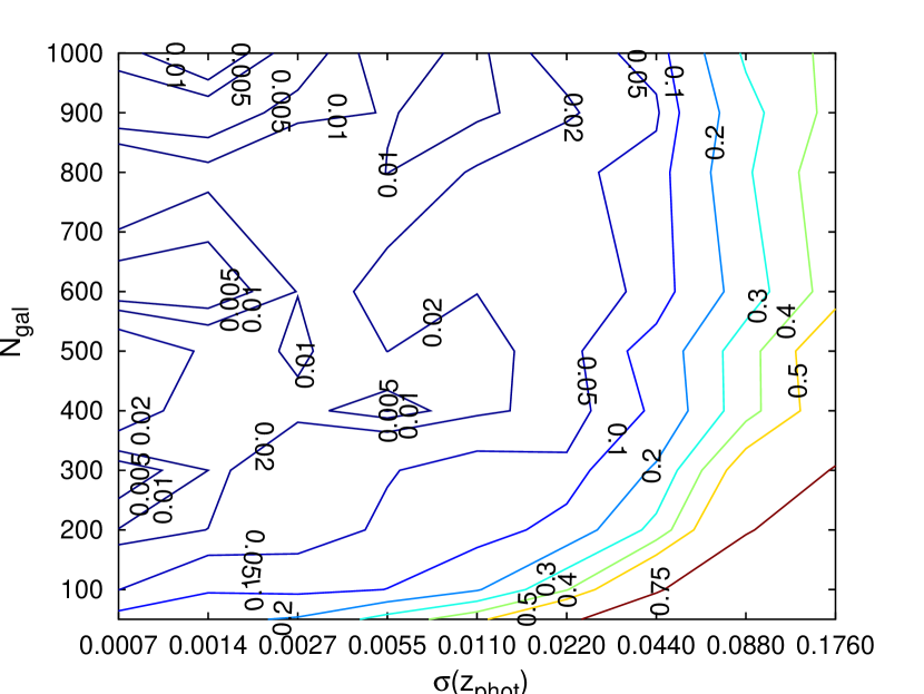
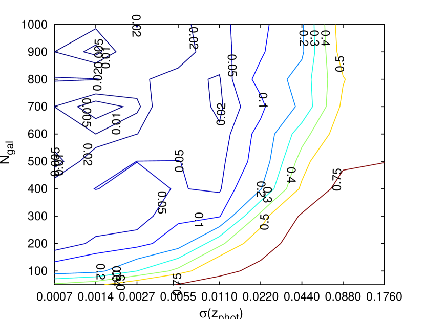
Figure 8 shows that increasing the survey area and redshift depth still further, to $\omega\approx 196$ deg² and $4<z<7$, would allow statistically similar results for weaker accuracy of the photometric redshifts and lower numbers of galaxies. An accuracy of $\sigma(z_{\mathrm{phot}})\,\lower 2.58334pt\hbox{$\buildrel<\over{\sim}$}\,0.02$ or $\sigma(z_{\mathrm{phot}})\,\lower 2.58334pt\hbox{$\buildrel<\over{\sim}$}\,0.01$, for $\Delta t=1$ $h^{-1}$ Gyr (upper panel) or $\Delta t=0.1$ $h^{-1}$ Gyr (lower panel), respectively, would give $p_{1}\,\lower 2.58334pt\hbox{$\buildrel<\over{\sim}$}\,0.05$.

Figure 8 also shows that for a sufficiently high number of galaxies, $N_{\mathrm{gal}}\,\lower 2.58334pt\hbox{$\buildrel>\over{\sim}$}\,900$, a photometric redshift accuracy of $\sigma(\Delta z_{\mathrm{phot}})\,\lower 2.58334pt\hbox{$\buildrel<\over{\sim}$}\,0.01$ would be sufficient for $p_{1}\,\lower 2.58334pt\hbox{$\buildrel<\over{\sim}$}\,0.01$, i.e. an expectation value of false rejection of about 1%. Most of the present interest in photometric redshift techniques is at lower redshifts, but high statistical accuracy in $z\sim 6$ photometric redshifts would clearly be useful for deep redshift topological lensing.

4 Conclusion

Over the next few decades, wide-angle surveys in the $z\sim 6$ redshift range will inevitably be performed. The results above indicate that with appropriate targetting and choices of observational parameter limits, the speed with which the $T^{3}$ candidate for the topology of the Universe can be rejected or detected can be optimised. For more specific observational strategies for particular telescope/instrument combinations, more detailed analyses could potentially be carried out by using detailed galaxy formation models, such as the hybrid $N$-body/semi-analytic simulations (Roukema et al. 1993; Roukema et al. 1997, 2001) that have been extensively developed to simulate detailed galaxy properties as a function of space and time (e.g., Hatton et al. 2003, and references thereof), including a specific focus on LAEs (e.g., Garel et al. 2012). More sophisticated combinations of existing observations, including the VVDS 1400+05 field within 16^∘ of the same southern axis and the VVDS 0226$-$04 field within 20^∘ of the corresponding northern axis (Table 4) along with simulated future observations, should also potentially yield several alternative strategies for topological lensing detection or rejection.

The total number of $L_{*}$ galaxies at $4\leq z\leq 7$, where $L_{*}$ is the characteristic luminosity of a Schechter function (Schechter 1976), is estimated to be $\phi_{*}\sim 3\times 10^{-3}$$h^{3}$ Mpc^-3 (e.g. Table 5, Bouwens et al. 2011). This gives about 3–8 million $L_{*}$ galaxies for the pairs of 100 deg² and 196 deg² fields simulated above, over $4.3<z<6.6$ and $4<z<7$, respectively. For the minimum $N_{\mathrm{gal}}\,\lower 2.58334pt\hbox{$\buildrel>\over{\sim}$}\,500$ or $N_{\mathrm{gal}}\,\lower 2.58334pt\hbox{$\buildrel>\over{\sim}$}\,400$ needed for achieving 5% expected confidence levels in the two field sizes, respectively (Sect. 3.2), surveys complete to $L\,\lower 2.58334pt\hbox{$\buildrel>\over{\sim}$}\,8.8L_{*}$ or $L\,\lower 2.58334pt\hbox{$\buildrel>\over{\sim}$}\,9.9L_{*}$, respectively, would find the required numbers of galaxies. Because the computing time for the above calculations scales roughly as $N_{\mathrm{gal}}^{4}$ for sufficiently high $N_{\mathrm{gal}}$ (since the heaviest computation is checking the list of possible quadruples; see Appendix B), simulations for surveys complete to $L\,\lower 2.58334pt\hbox{$\buildrel>\over{\sim}$}\,L_{*}$, i.e. for $N_{\mathrm{gal}}\,\lower 2.58334pt\hbox{$\buildrel>\over{\sim}$}\,10^{6}$, are clearly not practical without further filters added early in the successive filter algorithm.

Nevertheless, the most difficult aspect of predicting constraints on the model is the difference between precise cosmology and accurate cosmology. The dark energy parameter $\Omega_{\Lambda}$ is suspected by several cosmologists to be an artefact of using the FLRW metric (a homogeneous solution of the Einstein equation) rather than the physical average metric of the actually inhomogeneous Universe (e.g. Buchert & Carfora 2003; Buchert 2008; Célérier et al. 2010; Wiegand & Buchert 2010; Kolb 2011; Boehm & Rasanen 2013; Wiltshire et al. 2013; Buchert et al. 2013; Roukema et al. 2013). A significant confirmation of the $T^{3}$ hypothesis would provide a constraint on the inhomogeneous approach to cosmology, but this is unlikely to occur using an FLRW interpretation of the observational data if the time dependence of the FLRW metric parameters is too far from relativistically consistent formulae in the relevant redshift range (Larena et al. 2009). Some of the familiar FLRW relations may be algebraically valid in fully relativistic models, with an effective rather than a local physical interpretation (Buchert & Räsänen 2012), so detection of topological lensing might still be possible under the assumption of an FLRW metric.

Appendix A Combination of cosmological and peculiar velocities in the FLRW model

As derived in Synge (1960) and presented in Narlikar (1994) (see also Roukema 2010, and refs therein), the expansion redshift can be derived by parallel-transporting the four-velocity of the world line of a distant galaxy along a null geodesic (path of a photon) joining it to the observer. A fundamental observer (at rest with respect to the comoving spatial coordinate system) has zero peculiar velocity and a redshift of ${z}_{\mathrm{cosm}}$. The latter can be interpreted as a special-relativistic radial speed ${\beta}_{\mathrm{cosm}}$ in natural units, where

$$1+{z}_{\mathrm{cosm}} = \sqrt{\frac{1+{\beta}_{\mathrm{cosm}}}{1-{\beta}_{\mathrm{cosm}}}}$$ (12)

$$= \frac{1}{{\gamma}_{\mathrm{cosm}}(1-{\beta}_{\mathrm{cosm}})}$$

$$= {\gamma}_{\mathrm{cosm}}(1+{\beta}_{\mathrm{cosm}})$$

$$= \cosh{\phi}_{\mathrm{cosm}}+\sinh{\phi}_{\mathrm{cosm}}$$

$$= \mathrm{e}^{{\phi}_{\mathrm{cosm}}},$$

where ${\phi}_{\mathrm{cosm}}$ is the rapidity defined by ${\beta}_{\mathrm{cosm}}=:\tanh{\phi}_{\mathrm{cosm}}$, ${\gamma}_{\mathrm{cosm}}:=(1-{\beta}_{\mathrm{cosm}}^{2})^{-1/2},$ and ${\gamma}_{\mathrm{pec}}:=(1-{\beta}_{\mathrm{pec}}^{2})^{-1/2}.$ For a radial peculiar velocity of ${\beta}_{\mathrm{pec}}$ in natural units, the overall redshift $z$ can be calculated using Minkowski spacetime addition of the rapidities ${\phi}_{\mathrm{cosm}}$ and ${\phi}_{\mathrm{pec}}$, where ${\beta}_{\mathrm{pec}}=:\tanh{\phi}_{\mathrm{pec}}$, i.e. the overall rapidity is

$$\phi={\phi}_{\mathrm{cosm}}+{\phi}_{\mathrm{pec}},$$ (13)

since addition of four-velocity vectors at the same spacetime location is meaningful. Thus, similarly to Eq. (12), the overall redshift is given by

$$1+z = \mathrm{e}^{\phi}$$ (14)

$$= \mathrm{e}^{{\phi}_{\mathrm{cosm}}+{\phi}_{\mathrm{pec}}}$$

$$= (1+{z}_{\mathrm{cosm}})(1+{z}_{\mathrm{pec}}),$$

i.e.

$$z={z}_{\mathrm{cosm}}+{z}_{\mathrm{pec}}+{z}_{\mathrm{cosm}}{z}_{\mathrm{pec}}.$$ (15)

When $\max({z}_{\mathrm{cosm}},|{z}_{\mathrm{pec}}|)\ll 1$, this reduces to $z={z}_{\mathrm{cosm}}+{z}_{\mathrm{pec}}$ to first order in both redshifts.

For high-redshift astronomy, i.e. ${z}_{\mathrm{cosm}}>1$, the third term in the right-hand side of Eq. (15) is more significant than the second, contrary to popular belief that sets the third term to zero. Nevertheless, for $|{z}_{\mathrm{pec}}|\ll 1$, which is realistic even for low-redshift astronomy, Eq. (15) can be approximated to first order in ${\beta}_{\mathrm{pec}}$,

$$z\approx{z}_{\mathrm{cosm}}+{\beta}_{\mathrm{pec}}+{z}_{\mathrm{cosm}}{\beta}_{\mathrm{pec}}.$$ (16)

We ignore gravitational redshift here, since observations close to the Schwarzschild radius are unlikely in the case of interest. Parallel transport of the four-velocity (see Narlikar 1994) implies analogous relations to those above.

Figure 9: Confidence level calculation time in seconds for quadruple searches of (the equivalent of) 30 realisations for a single parameter set, as a function of the total number of galaxies $N_{\mathrm{gal}}$, for the simulations shown in Figs 7 and 8, for three different processor sets, as labelled. The times for the first processor set are halved to give the equivalent of four cores. Power-law fits to $N_{\mathrm{gal}}\geq 400$ are shown.

Appendix B Simulation benchmarking

Figure 9 shows that for sufficiently high $N_{\mathrm{gal}}$, the successive filter quadruple searches scale roughly as the fourth power of the number of simulated galaxies. From top to bottom as labelled, the power law best fits are proportional to $N_{\mathrm{gal}}^{4.2},$ $N_{\mathrm{gal}}^{4.1},$ and $N_{\mathrm{gal}}^{3.9},$ respectively. Parallelisation is via openmp.

References

- Aslanyan & Manohar (2012) Aslanyan, G., & Manohar, A. V. 2012, JCAP, 6, 3, [arXiv:1104.0015]
- Aurich (2008) Aurich, R. 2008, ClassQuantGra, 25, 225017, [arXiv:0803.2130]
- Aurich et al. (2008) Aurich, R., Janzer, H. S., Lustig, S., & Steiner, F. 2008, ClassQuantGra, 25, 125006, [arXiv:0708.1420]
- Aurich et al. (2005a) Aurich, R., Lustig, S., & Steiner, F. 2005a, ClassQuantGra, 22, 3443, [arXiv:astro-ph/0504656]
- Aurich et al. (2005b) Aurich, R., Lustig, S., & Steiner, F. 2005b, ClassQuantGra, 22, 2061, [arXiv:astro-ph/0412569]
- Aurich et al. (2010) Aurich, R., Lustig, S., & Steiner, F. 2010, ClassQuantGra, 27, 095009, [arXiv:0903.3133]
- Aurich et al. (2004) Aurich, R., Lustig, S., Steiner, F., & Then, H. 2004, ClassQuantGra, 21, 4901, [arXiv:astro-ph/0403597]
- Aurich et al. (2007) Aurich, R., Lustig, S., Steiner, F., & Then, H. 2007, ClassQuantGra, 24, 1879, [arXiv:astro-ph/0612308]
- Bennett et al. (2003) Bennett, C. L., Halpern, M., Hinshaw, G., Jarosik, N., Kogut, A., Limon, M., & et al 2003, ApJSupp, 148, 1, [arXiv:astro-ph/0302207]
- Bennett et al. (2013) Bennett, C. L., Larson, D., Weiland, J. L., Jarosik, N., Hinshaw, G., & et al 2013, ApJSupp, 208, 20, [arXiv:1212.5225]
- Bielewicz & Banday (2011) Bielewicz, P., & Banday, A. J. 2011, MNRAS, 412, 2104, [arXiv:1012.3549]
- Block (2012) Block, D. L. 2012, in Holder R. D., Mitton S., eds, Astrophysics and Space Science Library Vol. 395 of Astrophysics and Space Science Library, Georges Lemaître and Stigler’s Law of Eponymy. p. 89, [arXiv:1106.3928]
- Boehm & Rasanen (2013) Boehm, C., & Rasanen, S. 2013, JCAP, 09, 003, [arXiv:1305.7139]
- Bouwens et al. (2011) Bouwens, R. J. et al. 2011, ApJ, 737, 90, [arXiv:1006.4360]
- Buchert (2008) Buchert, T. 2008, Gen. Rel. Grav., 40, 467, [arXiv:0707.2153]
- Buchert & Carfora (2003) Buchert, T., & Carfora, M. 2003, Physical Review Letters, 90, 031101, [arXiv:gr-qc/0210045]
- Buchert et al. (2013) Buchert, T., Nayet, C., & Wiegand, A. 2013, PRD, 87, 123503, [arXiv:1303.6193]
- Buchert & Räsänen (2012) Buchert, T., & Räsänen, S. 2012, Annual Review of Nuclear and Particle Science, 62, 57, [arXiv:1112.5335]
- Caillerie et al. (2007) Caillerie, S., Lachièze-Rey, M., Luminet, J.-P., Lehoucq, R., Riazuelo, A., & Weeks, J. 2007, A&A, 476, 691, [arXiv:0705.0217v2]
- Célérier et al. (2010) Célérier, M., Bolejko, K., & Krasiński, A. 2010, A&A, 518, A21, [arXiv:0906.0905]
- Copi et al. (2007) Copi, C. J., Huterer, D., Schwarz, D. J., & Starkman, G. D. 2007, PRD, 75, 023507, [arXiv:astro-ph/0605135]
- Copi et al. (2009) Copi, C. J., Huterer, D., Schwarz, D. J., & Starkman, G. D. 2009, MNRAS, 399, 295, [arXiv:0808.3767]
- Copi et al. (2010) Copi, C. J., Huterer, D., Schwarz, D. J., & Starkman, G. D. 2010, Advances in Astronomy, 2010, 847541, [arXiv:1004.5602]
- Cornish et al. (1996) Cornish, N. J., Spergel, D. N., & Starkman, G. D. 1996, ArXiv Gen.Rel. & Quant.Cosm. e-prints, [arXiv:gr-qc/9602039]
- Cornish et al. (1998) Cornish, N. J., Spergel, D. N., & Starkman, G. D. 1998, ClassQuantGra, 15, 2657
- Davis et al. (2007) Davis, M., Guhathakurta, P., Konidaris, N. P., Newman, J. A., Ashby, M. L. N., & et al 2007, ApJL, 660, L1, [arXiv:astro-ph/0607355]
- de Sitter (1917) de Sitter, W. 1917, MNRAS, 78, 3
- Ducout et al. (2013) Ducout, A., Bouchet, F. R., Colombi, S., Pogosyan, D., & Prunet, S. 2013, MNRAS, 429, 2104, [arXiv:1209.1223]
- Findlay et al. (2011) Findlay, J. R., Sutherland, W. J., Venemans, B. P., Reyle, C., Robin, A. C., Bonfield, D. G., Bruce, V. A., & Jarvis, M. J. 2011, ArXiv e-prints, [arXiv:1111.3314]
- Friedmann (1923) Friedmann, A. 1923, Mir kak prostranstvo i vremya (The Universe as Space and Time). Petrograd: Academia
- Friedmann (1924) Friedmann, A. 1924, Zeitschr. für Phys., 21, 326
- Fujii & Yoshii (2011) Fujii, H., & Yoshii, Y. 2011, A&A, 529, A121, [arXiv:1103.1466]
- Fujii & Yoshii (2013) Fujii, H., & Yoshii, Y. 2013, ApJ, 773, 152, [arXiv:1306.2737]
- Gardner et al. (2006) Gardner, J. P., Mather, J. C., Clampin, M., Doyon, R., Greenhouse, M. A., Hammel, H. B., & et al 2006, Space Sci. Rev., 123, 485, [arXiv:astro-ph/0606175]
- Garel et al. (2012) Garel, T., Blaizot, J., Guiderdoni, B., Schaerer, D., Verhamme, A., & Hayes, M. 2012, MNRAS, 422, 310, [arXiv:1202.0610]
- Giacconi et al. (2001) Giacconi, R. et al. 2001, ApJ, 551, 624, [arXiv:astro-ph/0007240]
- Gundermann (2005) Gundermann, J. 2005, ArXiv Astrophysics e-prints, [arXiv:astro-ph/0503014]
- Hatton et al. (2003) Hatton, S., Devriendt, J. E. G., Ninin, S., Bouchet, F. R., Guiderdoni, B., & Vibert, D. 2003, MNRAS, 343, 75, [arXiv:astro-ph/0309186]
- Iovino et al. (2005) Iovino, A., McCracken, H. J., Garilli, B., Foucaud, S., Le Fèvre, O., Maccagni, D., & et al 2005, A&A, 442, 423, [arXiv:astro-ph/0507668]
- Key et al. (2007) Key, J. S., Cornish, N. J., Spergel, D. N., & Starkman, G. D. 2007, PRD, 75, 084034, [arXiv:astro-ph/0604616]
- Kolb (2011) Kolb, E. W. 2011, ClassQuantGra, 28, 164009
- Lachièze-Rey & Luminet (1995) Lachièze-Rey, M., & Luminet, J. 1995, Phys.Rep., 254, 135, [arXiv:gr-qc/9605010]
- Larena et al. (2009) Larena, J., Alimi, J.-M., Buchert, T., Kunz, M., & Corasaniti, P.-S. 2009, PRD, 79, 083011, [arXiv:0808.1161]
- Le Fèvre et al. (2003) Le Fèvre, O., Vettolani, G., Maccagni, D., Picat, J.-P., Garilli, B., & et al 2003, The Messenger, 111, 18
- Lehnert et al. (2010) Lehnert, M. D. et al. 2010, Nat., 467, 940, [arXiv:1010.4312]
- Lehoucq et al. (1996) Lehoucq, R., Lachièze-Rey, M., & Luminet, J.-P. 1996, A&A, 313, 339, [arXiv:gr-qc/9604050]
- Lehoucq et al. (1999) Lehoucq, R., Luminet, J.-P., & Uzan, J.-P. 1999, A&A, 344, 735, [arXiv:astro-ph/9811107]
- Lemaître (1927) Lemaître, G. 1927, Annales de la Société Scientifique de Bruxelles, 47, 49
- Lemaître (1931) Lemaître, G. 1931, MNRAS, 91, 483
- Luminet & Roukema (1999) Luminet, J., & Roukema, B. F. 1999, in Lachièze-Rey M., ed., NATO ASIC Proc. 541: Theoretical and Observational Cosmology. Publisher: Dordrecht: Kluwer, Topology of the Universe: Theory and Observation. p. 117, [arXiv:astro-ph/9901364]
- Luminet et al. (2003) Luminet, J., Weeks, J. R., Riazuelo, A., Lehoucq, R., & Uzan, J. 2003, Nat., 425, 593, [arXiv:astro-ph/0310253]
- Luminet (1998) Luminet, J.-P. 1998, Acta Cosmologica, XXIV-1, 105, [arXiv:gr-qc/9804006]
- Luminet (2006) Luminet, J.-P. 2006, Brazilian Journal of Physics, 36, 107, [arXiv:astro-ph/0501189]
- Luminet (2013) Luminet, J.-P. 2013, ArXiv e-prints, [arXiv:1305.6470]
- Maihara et al. (2001) Maihara, T., Iwamuro, F., Tanabe, H., Taguchi, T., Hata, R., & et al 2001, PASJ, 53, 25, [arXiv:astro-ph/0009409]
- Marecki et al. (2005) Marecki, A., Roukema, B. F., & Bajtlik, S. 2005, A&A, 435, 427, [arXiv:astro-ph/0412181]
- Mecke et al. (1994) Mecke, K. R., Buchert, T., & Wagner, H. 1994, A&A, 288, 697, [arXiv:astro-ph/9312028]
- Motohara et al. (2002) Motohara, K. et al. 2002, PASJ, 54, 315, [arXiv:astro-ph/0203320]
- Narlikar (1994) Narlikar, J. V. 1994, American Journal of Physics, 62, 903
- Niarchou & Jaffe (2007) Niarchou, A., & Jaffe, A. 2007, Physical Review Letters, 99, 081302, [arXiv:astro-ph/0702436]
- Picard (1884) Picard, E. 1884, Bull. Soc. Math. France, 12, 43, http://www.numdam.org/item?id=BSMF_1884__12__43_0
- Polsterer et al. (2012) Polsterer, K. L., Zinn, P.-C., & Gieseke, F. 2012, MNRAS, p. 10, [arXiv:1210.7071]
- Rebouças & Gomero (2004) Rebouças, M. J., & Gomero, G. I. 2004, Braz. J. Phys., 34, 1358, [arXiv:astro-ph/0402324]
- Refregier et al. (2010) Refregier, A., Amara, A., Kitching, T. D., Rassat, A., Scaramella, R., Weller, J., & Euclid Imaging Consortium 2010, ArXiv e-prints, [arXiv:1001.0061]
- Robertson (1935) Robertson, H. P. 1935, ApJ, 82, 284
- Roukema (1996) Roukema, B. F. 1996, MNRAS, 283, 1147, [arXiv:astro-ph/9603052]
- Roukema (2000) Roukema, B. F. 2000, Bull. Astr. Soc. India, 28, 483, [arXiv:astro-ph/0010185]
- Roukema (2010) Roukema, B. F. 2010, MNRAS, 404, 318, [arXiv:0911.1205]
- Roukema et al. (2008a) Roukema, B. F., Buliński, Z., & Gaudin, N. E. 2008, A&A, 492, 657, [arXiv:0807.4260]
- Roukema et al. (2008b) Roukema, B. F., Buliński, Z., Szaniewska, A., & Gaudin, N. E. 2008, A&A, 486, 55, [arXiv:0801.0006]
- Roukema & Kazimierczak (2011) Roukema, B. F., & Kazimierczak, T. A. 2011, A&A, 533, A11, [arXiv:1106.0727]
- Roukema et al. (2001) Roukema, B. F., Ninin, S., Devriendt, J., Bouchet, F. R., Guiderdoni, B., & Mamon, G. A. 2001, A&A, 373, 494, [arXiv:astro-ph/0105152]
- Roukema et al. (2013) Roukema, B. F., Ostrowski, J. J., & Buchert, T. 2013, JCAP, 10, 043, [arXiv:1303.4444]
- Roukema et al. (1997) Roukema, B. F., Peterson, B. A., Quinn, P. J., & Rocca-Volmerange, B. 1997, MNRAS, 292, 835, [arXiv:astro-ph/9707294]
- Roukema et al. (1993) Roukema, B. F., Quinn, P. J., & Peterson, B. A. 1993, in G. L. Chincarini, A. Iovino, T. Maccacaro, & D. Maccagni ed., Observational Cosmology: an International Symposium, Milano, Italy, 21–25 September 1992 Vol. 51 of Astronomical Society of the Pacific Conference Series, Spectral Evolution of Merging/Accreting Galaxies. p. 298
- Sarkar et al. (2011) Sarkar, D., Huterer, D., Copi, C. J., Starkman, G. D., & Schwarz, D. J. 2011, Astroparticle Physics, 34, 591, [arXiv:1004.3784]
- Schechter (1976) Schechter, P. 1976, ApJ, 203, 297
- Schmalzing & Buchert (1997) Schmalzing, J., & Buchert, T. 1997, ApJL, 482, L1, [arXiv:astro-ph/9702130]
- Schmalzing & Gorski (1998) Schmalzing, J., & Gorski, K. M. 1998, MNRAS, 297, 355, [arXiv:astro-ph/9710185]
- Shimasaku et al. (2006) Shimasaku, K. et al. 2006, PASJ, 58, 313, [arXiv:astro-ph/0602614]
- Spergel et al. (2003) Spergel, D. N. et al. 2003, ApJSupp, 148, 175, [arXiv:astro-ph/0302209]
- Starkman (1998) Starkman, G. D. 1998, ClassQuantGra, 15, 2529
- Starobinsky (1993) Starobinsky, A. A. 1993, Journal of Experimental and Theoretical Physics Letters, 57, 622
- Stevens et al. (1993) Stevens, D., Scott, D., & Silk, J. 1993, Physical Review Letters, 71, 20
- Synge (1960) Synge, J. 1960, Relativity: The General Theory. Amsterdam: North-Holland
- Taylor & Wheeler (1992) Taylor, E. F., & Wheeler, J. A. 1992, Spacetime physics - Introduction to special relativity (2nd edition)
- Uzan et al. (1999) Uzan, J.-P., Lehoucq, R., & Luminet, J.-P. 1999, A&A, 351, 766, [arXiv:astro-ph/9903155]
- van den Bergh (2011) van den Bergh, S. 2011, J. Roy. Ast. Soc. Canada, p. in press, [arXiv:1106.1195]
- Vernet et al. (2011) Vernet, J., Dekker, H., D’Odorico, S., Kaper, L., Kjaergaard, P., & et al 2011, A&A, 536, A105, [arXiv:1110.1944]
- Wiegand & Buchert (2010) Wiegand, A., & Buchert, T. 2010, PRD, 82, 023523, [arXiv:1002.3912]
- Williams et al. (2000) Williams, R. E., Baum, S., Bergeron, L. E., Bernstein, N., Blacker, B. S., & et al 2000, AJ, 120, 2735
- Williams et al. (1996) Williams, R. E. et al. 1996, AJ, 112, 1335, [arXiv:astro-ph/9607174]
- Wiltshire et al. (2013) Wiltshire, D. L., Smale, P. R., Mattsson, T., & Watkins, R. 2013, PRD, 88, 083529, [arXiv:1201.5371]