Recommending Given Names
Mining Relatedness of Given Names based on Data from the Social Web

Abstract

All over the world, future parents are facing the task of finding a suitable given name for their child. This choice is influenced by different factors, such as the social context, language, cultural background and especially personal taste. Although this task is omnipresent, little research has been conducted on the analysis and application of interrelations among given names from a data mining perspective.

The present work tackles the problem of recommending given names, by firstly mining for inter-name relatedness in data from the Social Web. Based on these results, the name search engine “Nameling” was built, which attracted more than 35,000 users within less than six months, underpinning the relevance of the underlying recommendation task. The accruing usage data is then used for evaluating different state-of-the-art recommendation systems, as well our new NameRank algorithm which we adopted from our previous work on folksonomies and which yields the best results, considering the trade-off between prediction accuracy and runtime performance as well as its ability to generate personalized recommendations. We also show, how the gathered inter-name relationships can be used for meaningful result diversification of PageRank-based recommendation systems.

As all of the considered usage data is made publicly available, the present work establishes baseline results, encouraging other researchers to implement advanced recommendation systems for given names.

1 Introduction

The choice of a given name is typically accompanied with an extensive search for the most suitable alternatives, at which many constraints apply. First of all, the social and cultural background determines, what a common name is and may additional imply certain habits, such as, e. g., the patronym. Additionally, most names bear a certain meaning or associations which, also depend on the cultural context.

Whoever makes the decision is strongly influenced by personal taste and current trends within the social context. Either by preferring names which are currently popular, or by avoiding names which most likely will be common in the neighborhood. Recently, public discussion of psychological effects associated with certain given names, which eventually may lead to social discrimination of individuals [31], increased the perception of responsibility of future parents, making the process of finding a given name even more involved.

Future parents are often aided by huge collections of given names which list several thousand names, ordered alphabetically or by popularity. With the first author’s need for a given name for his child, the idea arose to collect data from the “Social Web” in order to derive background information, popularity, interrelations and similarities of given names. The search engine “Nameling” [26] utilizes Wikipedia’s text corpus for interlinking names and the micro-blogging service Twitter for capturing current trends and popularity of given names. Nevertheless, the underlying rankings [27] and thus the search results are statically bound to the underlying co-occurrence graph obtained from Wikipedia and thus not personalized.

This work presents the task of recommending given names, applying approaches for distributional semantics and state-of-the-art recommender systems, such as user based collaborative filtering (UCF), item based collaborative filtering (ICF) and matrix factorization approaches. Additionally, the recommendation algorithm NameRank is presented, which is adopted from previous work on folksonomies [12], showing good performance in terms of prediction accuracy as well as runtime complexity.

The rest of the work is structured as follows: In Sec. 2, inter-name similarities are derived and evaluated. Sec. 3 presents the usage data of the Nameling search engine which is then used for evaluating name recommendation approaches. Then, in Sec. 4, different approaches for result diversification are discussed and evaluated.

2 Relatedness of Given Names

This section aims at discovering relations among given names, which can be used to aid future parents in searching and finding suitable names by means of ranking and recommendations techniques.

There are many reasons for names being related, ranging from phonetic similarity to common cultural context or similar “meaning”. With the rise of the Social Web, a whelm of data sources becomes available, interconnecting users and object information, either explicitly or implicitly [25]. In particular, given names are linked by social interactions of respective holder of the names as well as occurrences within heterogeneous, mostly unstructured data collections.

Ultimately, by leveraging data from online social networks, microblogging systems and encyclopedic background information, recommendation systems for given names may consider the user’s social context, cultural habits, personal taste and common popularity. In the following, we present a simple, yet powerful approach for mining interrelations among given names, which is based on co-occurrence networks.

Data Sources

For building co-occurrences networks of given names, we used the official Wikipedia data dump which is freely available for download and considered the English (date: 2012-01-05), French (2012-01-17) and German (2011-12-12) version separately. We additionally used the categorization of the affiliated Wiktionary project (English, French and German 2012-06-06), also available for download. As an additional source for user generated data, we considered the microblogging service Twitter. Using Twitter, each user publishes short text messages (called “tweets”). We used the data set introduced in [42], which comprises 476,553,560 tweets from 17,069,982 users, collected 2009/06 until 2009/12. Some effort was made to build up a comprehensive list of given names. In a semi-automatic way, a list of more than 30,000 names was collected. During the first months of the Nameling’s live time, additional names were proposed by users of the system, yielding a list of 36,434 given names.

2.1 Networks of Given Names

One of the most basic notions of relatedness between two given names can be observed, when they occur together in an atomic context of a given data collection. In case of Wikipedia, we counted such co-occurrences based on sentences and for Twitter based on tweets. We thus obtain for each data source $S\in\{\text{EN},\text{DE},\text{FR},\text{Twitter}\}$ (English, German and French Wikipedia as well as Twitter) an undirected weighted graph $G_{S}=(V_{S},E_{S})$ where $V_{S}$ denotes the subset of all observed names within $S$ and for names $u,v$ exists an edge $(u,v)\in E_{S}$ with weight $w(u,v)$, if $u$ and $v$ co-occurred in exactly $w(u,v)$ contexts. For example, the given names “Peter” and “Paul” co-occurred in 30,565 sentences within the English Wikipedia. Accordingly, there is an edge $(\text{Peter},\text{Paul})$ in $G_{\text{{EN}}}$ with corresponding edge weights.

Table 1 summarizes the high level statistics for all considered co-occurrence networks. As one would expect, all networks contain a giant connected component [32] which almost covers the whole corresponding node sets. The network obtained from the English Wikipedia is the most densely connected network whereas the network obtained from Twitter is the least densely connected.

Table 1: High level statistics for all co-occurrence networks.

	$|V|$	$|E|$	density	#wcc	largest wcc
$G_{\text{{EN}}}$	$27,121$	$24,461,988$	$0.067$	$2$	$27,119$
$G_{\text{{DE}}}$	$25,032$	$13,172,603$	$0.042$	$2$	$25,030$
$G_{\text{{FR}}}$	$25,237$	$17,446,139$	$0.055$	$1$	$25,237$
$G_{\text{Twitter}}$	$25,902$	$6,634,551$	$0.020$	$1$	$25,902$

Inter-Network Correlation Test

For assessing the pairwise structural interdependence of the different networks, we apply the quadradic assignment procedure (QAP) test [3, 4]. For given graphs $G_{1}=(V_{1},E_{1})$ and $G_{2}=(V_{2},E_{2})$ with $U\mathrel{\mathop{:}}=V_{1}\cap V_{2}\neq\emptyset$ and adjacency matrices $A_{i}$ corresponding to ${G_{i}}_{|U}$ ($G_{i}$ reduced to the common vertex set $U$), the graph covariance is given by

$$\mathop{cov}(G_{1},G_{2})\mathrel{\mathop{:}}=\frac{1}{n^{2}-1}\sum_{i=1}^{n}\sum_{j=1}^{n}(A_{1}[i,j]-\mu_{1})(A_{2}[i,j]-\mu_{2})$$

where $n\mathrel{\mathop{:}}=|U|$ and $\mu_{i}$ denotes $A_{i}$’s mean ($i=1,2$). Then $\mathop{var}(G_{i})\mathrel{\mathop{:}}=\mathop{cov}(G_{i},G_{i})$ leading to the graph correlation $\rho(G_{1},G_{2})\mathrel{\mathop{:}}=\frac{\mathop{cov}(G_{1},G_{2})}{\sqrt{\mathop{var}(G_{1})\mathop{var}(G_{2})}}.$

The QAP test compares the observed graph correlation $\rho_{0}$ to the distribution of resulting correlation scores obtained on repeated random row/column permutations of $A_{2}$. The fraction of permutations $\pi$ with correlation $\rho^{\pi}\geq\rho_{o}$ is used for assessing the significance of an observed correlation score $\rho_{o}$. Intuitively, the test determines (asymptotically) the fraction of all graphs with the same structure as $G_{2|U}$ having at least the same level of correlation with $G_{1|U}$.

Table 2a shows the pairwise correlation scores for all considered networks. The Wikipedia-based co-occurrence graphs shows the strongest correlation. For assessing the significance of the observed correlations, we repeatedly calculated the pairwise correlations on 1,000 corresponding randomly generated null models. For any pair of the considered networks, every randomly generated null model showed much lower correlation scores ($<10^{-3}$), which indicates statistical significance [3].

We conclude that the co-occurrence networks structurally correlate. Nevertheless, language specific deviations exist. For discovering relations on named entities, the corresponding language should therefore be considered. In the next section we will investigate, how structural similarity within the co-occurrence networks correlate with natural notions of relatedness among given names.

Table 2: Left: Pairwise graph correlation observed in the co-occurrence graphs. Right: Basic statistics for the different activities within the Nameling

	$G_{\text{{EN}}}$	$G_{\text{{DE}}}$	$G_{\text{{FR}}}$	$G_{\text{Twitter}}$
$G_{\text{{EN}}}$	-	$0.406$	$0.332$	$0.049$
$G_{\text{{DE}}}$	-	-	$0.303$	$0.020$
$G_{\text{{FR}}}$	-	-	-	$0.015$

(a)

	#Users	#Names
Enter	$35,684$	$16,498$
Click	$22,339$	$10,028$
Favorite	$1,396$	$1,558$

(b)

2.2 Mining for Relations from the Social Web

In this section, we focus on the question, whether structural similarity in the co-occurrence networks from Section 2.1 gives rise to a notion of relatedness which implies relationships the user might be interested in. For evaluating and comparing different similarity metrics, we need a “reference” notion of relatedness for the considered names to be used as “ground truth”. For given names, there is no generally accepted reference relation. We therefore apply the approach of using an external data source which we assume as a valid “gold standard”. We argue that the categories assigned to names in Wiktionary are a good basis, as they are manually assigned and have a direct connection to concepts users associate with given names (such as gender and cultural context). We finally chose cosine similarity for calculating a reference similarity score, which is broadly accepted for various applications. For the sake of a concise presentation, we restrict our analysis in this chapter to the network obtained from the English Wikipedia and from Twitter.

Vertex Similarities

Subsequently, we only consider the two similarity functions which yielded the most promising results. For the discussion and evaluation of broader range of similarity metrics, refer to [29]. The Jaccard coefficient measures the fraction of common neighbors. For weighted networks, we also consider its weighted variant [30]. The cosine similarity measures the cosine of the angle between the corresponding rows of the adjacency matrix, where we consider both its weighted and unweighted variant.

For obtaining a reference relation on the set of given names, we collected all corresponding category assignments from Wiktionary. We thus obtained for each of 10,938 given names a respective binary vector, where each component indicates whether the corresponding category was assigned to it (in total 7,923 different categories and 80,726 non-zero entries). We laxly denote these category assignments as “semantic” properties and accordingly the induced similarity as “semantic similarity” of names.

Neighborhood & Similarity

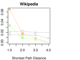
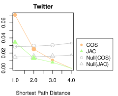
As a first analysis of the interdependence of a name’s position within the co-occurrence network and its category assignment in Wiktionary, we consider for pairs of names their respective shortest path distance relative to their reference similarity. Considering the co-occurrence networks obtain from Wikipedia and Twitter separately, we calculate the average corresponding similarity score for every shortest path distance $d$ and every pair of names $u,v$ with a shortest path distance $d$. To rule out statistical effects, the same calculations are repeated at which the correspondence of names within the network and the category assignment is randomly shuffled. Fig. 1 shows the results for the cosine similarity together with the Jaccard coefficient. In both networks, the similarity of node pairs tends to decrease monotonically with the respective shortest path distance, where direct neighbors are in average more similar than randomly chosen pairs (referring to the null model baseline) and pairs at distance two are already less similar than expected by chance.

Figure 1: Semantic relatedness vs. shortest path distance in the co-occurrence networks.

Structural & Semantical Similarity

The interplay of shortest path distance and semantic similarity of names indicates that the structural context of a name within the co-occurrence network is correlated with its semantic properties.

We now compare different vertex similarity metrics with respect to their ability to capture semantic similarity of names. In detail, we calculate for any pair $u,v$ of names in the co-occurrence network (which have a category assignment) the cosine similarity $\mathop{C\!O\!S}(u,v)$ based on the respective category assignment vectors as well as any of the considered vertex similarity metrics $s(u,v)$. As the number of data points $(\mathop{C\!O\!S}(u,v),s(u,v))$ grows quadratically with the number of names, we grouped the co-occurrence based similarity scores in 1,000 equidistant bins and calculated for each bin the average cosine similarity based on category assignments. Figure 2 shows the results for Wikipedia and Twitter separately.

Figure 2: Similarity based on name categories in Wiktionary vs. vertex similarity in the co-occurrence-networks (weighted and unweighted).

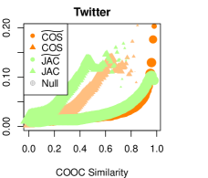
Notably, all considered similarity metrics capture a positive correlation between similarity in the co-occurrence network and similarity between category assignments to names. But significant differences between the underlying co-occurrence networks and the applied similarity functions can be observed. As for Wikipedia, the cosine similarity shows similar characteristics in its weighted and unweighted variant but for higher structural similarity scores the weighted variant is more consistent with the semantic similarity of names. Considering the Jaccard coefficient, the unweighted variant is more consistent with the reference similarity then its unweighted variant.

As for Twitter, both cosine similarity and the Jaccard coefficient are more consistent with the reference similarity for lower and average structural similarity scores. For higher structural similarity, the weighted cosine similarity shows strong correlations with the reference relation.

Summing up, edge weights without further pre-processing may significantly decrease the performance of a similarity metric with respect to its ability to capture semantic similarity of names. Furthermore, no clearly best structural similarity can be deduced from the conducted experiments. Nevertheless, correlations between structural and semantic similarity can be observed at all consistent vertex similarity functions.

3 Recommending Given Names

The results presented in the previous section indicate correlations between semantic relatedness among given names and structural similarity within co-occurrence networks obtained from different data sources.

We now turn our focus towards systems for personalized name recommendations, leveraging the usage data which accrued at Nameling’s log files. We firstly summarize the considered usage data and analyze the emerging networks of given names. We then briefly summarize different state-of-the-art recommendation systems and present our own recommendation approach. All considered recommendation systems are finally evaluated and compared with respect to their prediction accuracy.

3.1 Preliminaries

Throughout this section, we utilize $u,v$ and $i,j$ interchangeably as placeholder or index variables to denote users and items (i. e., names) respectively. We denote the set of users with $\mathcal{N}$ and the set of items with $\mathcal{M}$, denoting the number of users with $n\mathrel{\mathop{:}}=|\mathcal{N}|$ and the number of names with $m\mathrel{\mathop{:}}=|\mathcal{M}|$.

The context of our work is given by Nameling, a search and recommendation system for given names, where a user $u$ might express interest in name $i$, either by entering the name directly in a search mask, click on a name or add a name to the personal list of favorite names. We denote $u$’s expressed affiliation with $i$ by $r_{ui}^{\emph{Enter}{}}$, $r_{ui}^{\emph{Click}}$ and $r_{ui}^{\emph{Favorite}}$, respectively. All user-name affiliations are aggregated in the corresponding binary user-name matrices $R^{\emph{Enter}{}}$, $R^{\emph{Click}}$ and $R^{\emph{Favorite}}$. Whenever the corresponding activity class is irrelevant or determined by the context, we drop the superindex. Furthermore we consider the set $\mathcal{M}_{u}\mathrel{\mathop{:}}=\{j\in\mathcal{M}\mid r_{uj}>0\}$ of all names $j$ which user $u$ is affiliated with as well as the set $\mathcal{N}_{i}\mathrel{\mathop{:}}=\{v\in\mathcal{N}\mid r_{vi}>0\}$ of all users $v$ who are affiliated with the $i$th given name.

Please note that we consider binary user-name affiliations, i. e., $r_{ui}\in\{0,1\}$ where a zero value may either indicate that user $u$ is not interested in $i$, has not yet expressed her/his affiliation or is just unaware of $i$. A positive value of $r_{ui}$ on the other hand only in the case of adding a name to the personal list of favorites clearly indicates that $u$ likes $i$. The reason for entering or clicking on a name might also just be curiosity.

Recommending given names for a user $u$ based on a given user-name matrix $R$ corresponds to predicting $u$’s affiliation with any name $i\in\mathcal{M}\setminus\mathcal{M}_{u}$ which we denote with $\hat{r}_{uj}$. Most recommendation systems determine for each such user-item pair a score which reflects the recommender’s confidence about positive affiliation. Recommending $k$ names for $u$ is achieved by taking the top $k$ names from the thus ordered list of names. For a recommendation system Rec, we denote the ordered list of $k$ recommended names for user $u$ with $\text{Rec}^{k}(u)$ and write $\text{Rec}(u)$ to denote Rec’s ranking of all names for $u$, based on the recommender’s scoring function.

For assessing the prediction accuracy of a recommendation system, we process each user $u$ separately and select for evaluation a subset $\emph{Test}(u)\subset\mathcal{M}_{u}$. Recommendations for $u$ are then calculated on $\tilde{R}$ which is element-wise given by

$$\tilde{r}_{vj}\mathrel{\mathop{:}}=\begin{cases}0,&\text{if }v=u\text{ and }j\in\emph{Test}(u)\\ r_{vj},&\text{otherwise.}\end{cases}$$

We consider several metrics for scoring a recommendation system’s prediction accuracy:

Precision/Recall

Precision and recall are metrics originating from the evaluation of information retrieval systems, given by

$$\text{Precision}{{}^{k}\!(u)} \mathrel{\mathop{:}}= \frac{|\text{Rec}^{k}(u)\cap\emph{Test}(u)|}{k}$$

$$\text{Recall}{{}^{k}\!(u)} \mathrel{\mathop{:}}= \frac{|\text{Rec}^{k}(u)\cap\emph{Test}(u)|}{|\emph{Test}(u)|}$$

We interchangeably also write Precision@k and Recall@k to denote the average scores over all users $u\in\mathcal{N}$.

Average Precision/MAP

The mean average precision is a metric for obtaining a single value performance score for a recommendation system Rec considering all recommended names for all users:

$$\text{MAP}\mathrel{\mathop{:}}=\frac{1}{n}\sum_{u=1}^{n}\text{AveP}(u)$$

where the average precision is given by

$$\text{AveP}(u)\mathrel{\mathop{:}}=\frac{1}{|\mathcal{M}_{u}|}\sum_{k=1}^{|\mathcal{M}_{u}|}[\text{Precision}{{}^{k}\!(u)}\cdot\delta^{k}(u)]$$

and $\delta^{k}\!(u)=1$, iff the recommended element at rank $k$ is a relevant name (that is $\text{Rec}(u)[k]\in\emph{Test}(u)$). Refer to [40] for more details.

Normalized Discounted Cumulative Gain

The basic idea of the discounted cumulative gain metric (DCG) is that relevant items at higher ranking positions should be penalized. Typically, the penalization factor scales inverse logarithmically with the position in the list of recommended items:

$$\text{DCG}{{}^{k}}(u)\mathrel{\mathop{:}}=\sum_{i=1}^{k}\frac{2^{\delta^{i}(u)}-1}{\log_{2}(i+1)}$$

For normalizing the DCG score across recommendations for different users, the DCG score is considered relative to the best possible DCG score for the considered user, called the ideal score IDCG, resulting in

$$\text{NDCG}{{}^{k}}(u)\mathrel{\mathop{:}}=\frac{\text{DCG}^{k}(u)}{\text{IDCG}^{k}(u)}$$

For maximal $k$ we drop the index and write NDCG. Please note hat we restrict our discussion to the binary case.

Test of Significance

For comparing the prediction accuracy of different recommendation systems, typically the average of some evaluation metric is compared. Due to the sensitivity of the average towards outliers such a comparison may often lead to erroneous conclusions. For further comparison the distribution of the respective evaluation metric should be taken into account too, e. g., in order to apply some statistical test for assessing the significance of the observed difference.

We apply the simple sign test for assessing, whether a recommendation system $A$ significantly outperforms recommendation system $B$, relative to some per user evaluation metric. For this purpose, we count the number $n_{A}$ of users where $A$ yields better scores than $B$ and inversely $n_{B}$. We thereby ignore all users with equal evaluation scores. The sign test assesses the significance $p$ of an observed outcome $n_{A}$ and $n_{B}$ by estimating the probability that $A$ is not truly better than $B$ with the probability that $n_{A}$ out of $n\mathrel{\mathop{:}}=n_{A}+n_{B}$ uniform Binomial tries succeed:

$$p=\left(\frac{1}{2}\right)^{n}\sum_{i=n_{A}}^{n}\frac{n!}{i!(n-i)!}$$

Please refer to [36, 6] for further details and more advanced hypothesis tests for comparing recommendation systems. Please note that we only assess the significance of selected results in order to reduce the impact of correcting the influence of multiple testings (e. g., Bonferroni correction).

3.2 Usage Data

For our analysis and evaluation, we considered the Nameling’s activity log entries within the time range 2012-03-06 until 2012-08-10. In the following, we firstly describe the collected usage data, analyze properties of emerging network structures and finally compare interrelations between the different networks.

In total, 38,404 users issued 342,979 search requests. Subsequently, we differentiate between activities where a user manually entered a given name (“Enter”), followed a link to a name within a result list (“Click”) or added a given name the list of favorite names (“Favorite”). Table 2b summarizes high level statistics for these activity classes, showing, e. g., that $35,684$ users entered $16,498$ different given names.

For analyzing how different users contribute to the Nameling’s activities, Figure 3 shows the distribution of activities over the set of users, separately for Enter, Click and Favorite requests. Clearly, all activities’ distributions exhibit long tailed distributions, that is, most users entered less than 20 names but there are also users with more than 200 requests.

Figure 3: Number of users per query count for Enter, Click and Favorite activities.

In order to assess the interdependence of name contexts established by search queries within the Nameling and co-occurrences within Wikipedia, we further constructed for each activity class $C\in\{\text{\emph{Enter}},\text{\emph{Click}},\text{\emph{Favorite}}\}$ a corresponding weighted projection graph $G_{C}$, where an edge $(i,j)$ exists with weight $k$, if $k$ users searched for both names $i$ and $j$). Table 3 summarizes various high level network statistics for all considered projection graphs. All projection graphs encompass a giant connected component [32], giving rise to a notion of relatedness among names.

Table 3: High level statistics for all considered projection graphs with the number of weakly connected components #wcc and largest weakly connected components lwcc.

	$|V|$	$|E|$	#wcc	lwcc	$D$
$G_{\text{\emph{Enter}}}$	$15,992$	$996,930$	$72$	$15,834$	$7$
$G_{\text{\emph{Click}}}$	$9,665$	$2,633,220$	$79$	$9,465$	$10$
$G_{\text{\emph{Favorite}}}$	$1,365$	$60,124$	$23$	$1,306$	$7$

Please note that these usage graphs themselves can be used for calculating similarity among given names, e. g., by applying the same similarity metrics as discussed for the co-occurrence graphs.

For assessing the interdependence of the name contexts established by the different co-occurrence networks from Sec. 2.1 and those emerging from Nameling’s query logs, we apply again the quadradic assignment procedure test (cf. Sec. 2.1). Table 4 shows the pairwise correlation scores for all considered networks.

Table 4: Graph level correlations for all pairs of considered networks. All observed correlations are significant according to the quadradic assignments procedure (QAP).

	$G_{\text{\emph{Enter}}}$	$G_{\text{\emph{Click}}}$	$G_{\text{\emph{Favorite}}}$	$\text{Wiki}^{DE}$	$\text{Wiki}^{EN}$	$G_{\text{Twitter}}$
$G_{\text{\emph{Enter}}}$	$-$	$0.466$	$0.370$	$0.138$	$0.054$	$0.0004$
$G_{\text{\emph{Click}}}$		$-$	$0.364$	$0.110$	$0.056$	$0.0002$
$G_{\text{\emph{Favorite}}}$			$-$	$0.040$	$0.032$	$0.0038$

Again, correlations are more pronounced within a system (e. g., $0.466$ for the $G_{\text{\emph{Enter}}}$ and $G_{\text{\emph{Click}}}$). But the graph level correlations for networks obtained from the Nameling exhibit significantly higher correlation scores for the co-occurrence network obtained from the German Wikipedia, indicating that the dominance of German users has an impact on the emerging name contexts within the search based networks which are more related to the accordingly language dependent network structure within the co-occurrence network from Wikipedia. Finally, the correlation scores for the Twitter based co-occurrence networks shows the least magnitude, though still signficant for $G_{\text{\emph{Enter}}}$ and $G_{\text{\emph{Favorite}}}$ in terms of the QAP test ($p<0.05$).

Summing up, we conclude that users accessing a name search engine like Nameling are implicitly establishing name contexts which differ from those, obtained from encyclopedic data sources, such as Wikipedia. These user centric name contexts are more likely to reflect the user’s taste and personal preference and accordingly may be used for generating personalized name recommendations.

3.3 The Recommendation Task

The choice of the given name is one of the first important decision future parents have to make. Many influencing factors have an impact on this decision process, such as, e. g., cultural background, current trends and personal taste. Typically, large collections of given names with additional background information for the corresponding names are at hand, either in the form of a lexicographical book or a specialized web site. Where a search engine for given names allows the user to browse through the list of names ordered by some notion of relevance, a recommendation system suggests a small personalized list of names which the user might be interested in.

Different constraints can apply to the list of recommended names, notably depending on the amount of background information available. Given names from the user’ ego-network of some on-line social network, e. g., could be ignored (assuming the user knows the given names of her or his friends), or, a certain diversity of names requested, as there is not desirable to present the user, e. g., just different variants of a single name. Each of such constraint influences the assessment of the quality of a recommendation system. Accordingly, there is no single valid evaluation protocol. Below, we present the evaluation protocol we applied for establishing baseline results for the quality of recommendation systems for given names.

Evaluation Protocols

The evaluation of a recommendation system is strictly dependent on the targeted objective [36]. Ultimately, only an appropriate comparative live evaluation of different recommendation systems can comprehensively assess the performance of such systems. In this section, we focus on the prediction accuracy relative to a publicly available activity log file from Nameling as presented in Section 3.2.

For this purpose, we process each user $u$ separately and remove from the set of entered search names Enter$(u)$ a subset Test$(u)$ for evaluation. We then use all activity data without the selected evaluation data for calculating recommendations and assess the prediction accuracy relative to Test$(u)$. We applied different strategies for selecting the evaluation set Test$(u)$, each of which suitable for examining certain research questions:

TakeKIn:

Test$(u)$ is randomly sampled with size $|\emph{Enter}{(u)}|-k$.

LeaveKOut:

Test$(u)$ is randomly sampled with size $k$.

TakeFirstIn:

Test$(u)$ consists of the last $|\emph{Enter}{(u)}|-k$ names the user $u$ has entered. Name recommendations are therefore based on the first $k$ names.

LeaveLastOut:

Test$(u)$ consists of the last $k$ names the user $u$ has entered.

Whenever results among different number of known names $k\leq N_{\max}$ are compared, we additionally removed $N_{\max}-k$ names from the user’s test set $\emph{Test}{(u)}$ to ensure that results for different values of $k$ are comparable and not determined through varying sizes of $\emph{Test}{(u)}$.

Please note that we only used the set of directly entered names (Enter) for evaluation and did not use the combination of Enter and Favorite events for evaluation, as these interrelations among names have a strong bias induced by the ranking function which was implemented in Nameling [26].

Evaluation Metrics

Various metrics for assessing the prediction accuracy of recommendation systems exist and the choice of the applied metric depends, among others, on the application context. Firstly, global metrics like MAP and NDCG summarize the prediction performance of all recommended items, whereas prefix metrics like Precision@$k$ and NDCG@$k$ only consider the first $k$ recommended items.

For the present work, we differentiate the recommendation task from searching by restricting recommendations to the corresponding top $k$ items, giving favor to Precision@$k$ and NDCG@$k$, whereof the latter accounts for the ordering of the recommended items within the top $k$ positions. For reference though, we also consider MAP and NDCG. When comparing different recommendation systems based on the corresponding MAP scores, special care has to be taken if one of the recommendation systems fails to generate rankings for all items. Consider, e. g., the PageRank based NameRank and user based collaborative filtering UCF. By construction, NameRank assigns weights to all names, whereas UCF cannot infer weights for names which are not connected to one of the queried user’s search names. Now, even for very low weights, relevant names are considered for calculating the average precision score which may degrade MAP significantly (due to the sensitivity of average towards outliers).

We argue that the fairest handling of such situations is to virtually place all $\ell$ relevant names for a user $u$ which an recommendation system Rec failed to recommend, at the end of $\text{Rec}(u)$.

3.4 Experimentation

This section focuses on the evaluation of the prediction accuracy of different recommendation systems. On the one side, the obtained results are a basis for deciding which recommendation system should be used for recommending given names in a corresponding application. On the other side, we thereby establish baseline results for the task of recommending given names which serve as a reference for developing and evaluating new approaches.

3.5 Applied Recommender Systems

Subsequently, we shortly summarize each considered recommendation system and introduce according abbreviations which we henceforth use for identifying individual recommendation systems.

User based CF (UCF):

Adopting the weighted sum approach for user based collaborative filtering [38] to the binary case (a user searched or searched not for a given name), we set

$$\text{UCF}(u,i)\mathrel{\mathop{:}}=\sum_{v\in\mathcal{N}_{i}}\mathop{S\!I\!M}(u,v).$$

For the nearest neighbor approach, only the top $N$ similar users to $u$ are considered in the summation.

For recommending $k$ names to user $u$, the top $k$ names, ordered descending by $\text{UCF}(u,*)$, are determined (ignoring names $j$ with ${r}_{uj}>0$).

Item based CF (ICF):

Adopting the weighted sum approach in [34] to the binary case, we set:

$$\text{ICF}(u,i)\mathrel{\mathop{:}}=\frac{\sum_{j\in\mathcal{M}_{u}}\mathop{S\!I\!M}(i,j)}{\sum_{j\in\mathcal{M}}\mathop{S\!I\!M}(i,j)}.$$

For recommending $k$ names to user $u$, the top $k$ names ordered descending by $\text{ICF}(u,*)$ are determined (ignoring names $j$ with ${r}_{uj}>0$).

PPR/PPR+

The preferential PageRank similarity is based on the well known PageRank [1] algorithm. For a $m\times m$ column stochastic adjacency matrix $A$ and damping factor $\alpha$, and uniform preference vector $\vec{p}\mathrel{\mathop{:}}=(1/m,\ldots,1/m)$, the global PageRank vector $\vec{w}\mathrel{\mathop{=}}:\mathop{P\!R}$ is given as the fixpoint of the following equation:

$$\vec{w}=\alpha A\vec{w}+(1-\alpha)\vec{p}$$

In case of the preferential PageRank for a given set of nodes $\mathcal{I}$, only the corresponding components of the preference vector are set and we set accordingly $\mathop{P\!P\!R}(\mathcal{I})$ to the fixpoint of the above equation with

$$p_{i}\mathrel{\mathop{:}}=\begin{cases}\frac{1}{|\mathcal{I}|},&\text{if }i\in\mathcal{I}\\ 0,&\text{otherwise.}\end{cases}$$

As a new item based recommendation approach we propose NameRank (for brevity abbreviated with $\mathop{P\!P\!R\!+}$), which is an adoption of the idea presented in [12], where the global PageRank score $\mathop{P\!R}$ is subtracted from the preferential PageRank score in order to reduce frequency effects and set

$$\mathop{P\!P\!R\!+}(\mathcal{I})\mathrel{\mathop{:}}=\mathop{P\!P\!R}(\mathcal{I})-\mathop{P\!R}.$$

For recommending $k$ names to user $u$, we calculate $\vec{w}\mathrel{\mathop{:}}=\mathop{P\!P\!R\!+}(\mathcal{M}_{u})$ on the column stochastic adjacency matrix derived from $G_{\emph{Enter}}$ (cf. Sec. 2) and recommend the top $k$ names ordered descending by $\vec{w}$, thereby ignoring names $j$ with ${r}_{uj}>0$.

Please note that we show results obtained by averaging the rankings from individual query names, i. e.,

$$\frac{1}{|\mathcal{I}|}\sum_{j\in\mathcal{I}}\mathop{P\!P\!R\!+}(\{j\})$$

which showed the same results as $\mathop{P\!P\!R\!+}(\mathcal{I})$.

WRMF

The weighted matrix factorization method [13] is designed to deal with implicit feedback scenarios like the our evaluation setting described in 3.3. The observed user-item interactions $r_{ui}$ are interpreted as indicators of user $u$’s preference for item $i$ which is associated with a certain level of confidence, depending on the amount of observed interactions. Unobserved interactions $\hat{r}_{ui}$ are predicted by building a factor model of the user-item matrix $R$ via an regularized learning method with alternating least squares optimization.

MostPopular

The MostPopular recommendation approach predicts for all users the most popular names, i. e., the top $k$ names ordered decreasing by frequency.

Random

The Random recommendation approach randomly selects $k$ names which the user has not searched before.

The item-based and user-based collaborative filtering as well as the MostPopular approaches were implemented using the machine learning library Mahout . We evaluated various similarity metrics, showing here results for the Log-Likelihood similarity [7] which outperformed the others. The PageRank-based approaches $\mathop{P\!P\!R}$ and $\mathop{P\!P\!R\!+}$ are implemented using the eigen  library for matrix operations. For WRMF we applied the implementation of the myMediaLite [9] library with the corresponding default parametrization.

We also considered the Bayesian personalized ranking approach for matrix factorization [33], additionally with soft-margin optimization as proposed in [41] as implemented in the myMediaLite recommendation library. But the obtained result showed worse prediction performance than the simple MostPopular recommendation approach and are therefore excluded from the presentation below for clarity.

Evaluation Data

For evaluating the prediction accuracy of the considered recommendation systems, we applied the different evaluation protocols described in Section 3.3 for $k=1,\ldots,N_{\max}$ with $N_{\max}\mathrel{\mathop{:}}=10$. To assure that for every user $u$ there are at least five names available for testing and prediction, respectively, we restricted our evaluation to users who entered more than 14 different names (that is, $|\emph{Enter}{(u)}|\geq 15$), leaving 1,230 users for evaluation. Please note that we neither considered the set Click$(u)$ of names which the user clicked on nor the set Favorite$(u)$ which the user added to the list of favorite names, as these data sets are strongly biased by the ranking which was implemented in Nameling’s search back-end.

3.6 Results

We now present our results on the prediction accuracy of the considered recommendation systems. We firstly present the results for the TakeKIn and LeaveKOut experiments where the results are obtained relatively to the number of names and finally the results of the TakeFirstIn and LeaveLastOut experiments, where results are obtained relative to the chronologically ordered first names of a user’s search history.

TakeKIn

This experiment aims at comparing the impact of personalization on the prediction accuracy of the different recommendation systems. In particular we want to examine…

• …whether and to which extend the performance of a recommendation system benefits from an increasing number of known names (i. e., increasing $k$).

• …whether for new users with only few known names, different recommendation systems perform best than for those users with a large search history.

For this purpose, we applied the TakeKIn evaluation protocol as described in Section 3.3 For eliminating the influence of certain selections of known names, we repeatedly sampled (25 times) for each user the set of $k$ known names and averaged the resulting evaluation scores. Furthermore, we removed $N_{\max}-k$ names from the user’s test set $\emph{Test}{(u)}$ to ensure that results for different number of known names $k$ are comparable and not determined through varying sizes of $\emph{Test}{(u)}$ for different $k$.

Figure 4 shows the obtained results for Precision@5, NDCG@5 and MAP. Please note that we didn’t include the random baseline results into Figure 4 for clarity, as all corresponding evaluation scores were two magnitudes below the worst result of the other recommenders.

(a)

(b)

(c)

Figure 4: Precision accuracy of the different recommendation systems, relative to varying number of known names per user. For clarity of presentation the random baseline was omitted which lies strictly below $10^{-3}$ for all metrics.

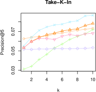
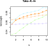
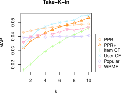
We begin with a discussion of some general observations. Firstly, all obtained performance scores are low in magnitude, indicating that given names are hard to predict based on the user’s search history. One of the key difficulties in such implicit feedback data is due to the indistinguishable intent of search requests [13]: A user might search for a name because the user likes the name, or the user might search for names he doesn’t like and just wants to explore the names neighborhood. Equally, the fact that a user did not search for a certain name might either express that the user dislikes the name, was not aware of the name or just did not search for the given name until now but eventually will.

Figure 5 exemplarily presents the distribution of the Precision@5 and MAP scores for $\mathop{P\!P\!R\!+}$ with ten known names, showing that the low scores are due to a highly skewed distribution where for most users no or only few relevant names are predicted. This, on the other hand, emphasizes the importance of additional analysis beside calculating average prediction metrics, as the average over skewed distributed values is sensitive to outliers. Nevertheless, the considered performance metrics consistently assess the impact of an increasing number of known names for all considered recommendation systems.

Figure 5: Distribution of the Precision@5 and MAP scores for $\mathop{P\!P\!R\!+}$ with ten known names.

For a more formal analysis of the consistency among the considered performance metrics, we assessed the prediction accuracy of each considered recommendation setting (in total 1435 models) with every performance metric, respectively averaged over all users. We thus obtained for each metric a ranking on all models, among which we calculated Kendall’s $\tau$ rank correlation coefficient. Table 5 shows the calculated correlation scores. Notably, all metrics but NDCG@10 show a very high correlation, supporting the observed consistent assessment of different recommendation systems with varying number of known names in Figure 4.

Table 5: Correlations between the different evaluation metrics averaged for each model separately.

	Precision@5	Precision@10	Recall@5	Recall@10	NDCG@5	NDCG@10	MAP
Precision@5	-
Precision@10	0.94	-
Recall@5	0.89	0.87	-
Recall@10	0.85	0.88	0.94	-
NDCG@5	0.94	0.90	0.86	0.82	-
NDCG@10	0.37	0.38	0.34	0.34	0.36	-
MAP	0.79	0.79	0.79	0.79	0.81	0.35	-

We now turn our focus to the discussion of the performance scores for the different recommendation systems in Figure 4. The most popular recommendation approach shows a relative good performance, as expected independent of the number $k$ of known names. This is therefore a suitable baseline for assessing other recommendation systems’ performance scores. All other considered methods benefit from increasing $k$. In particular the item based collaborative filtering shows a linearly increasing performance scores, thereby showing worse performance than the most popular baseline for lower $k$. Except for $k\leq 2$, the user based collaborative filtering approach shows the highest performance scores.

As for $\mathop{P\!P\!R}$ and $\mathop{P\!P\!R\!+}$, the former shows better performance for lower $k$ (even outperforming user based collaborative filtering) whereas the latter steadily increases with the number of known names. Please note that this is in line with the intention for the construction of $\mathop{P\!P\!R\!+}$: the plain preferential PageRank is strongly influenced by global frequencies which are reduced by subtracting the global PageRank (cf. Section 3.5). As the popular (i. e., most frequent names) are already a relative good recommendation, the influence of global frequencies is desirable if only few names of a user are known.

Finally WRMF also shows increasing prediction accuracy with increasing number known names.

LeaveKOut

In this experimental setup, as much of the user $u$’s search history as possible is used for predicting the user’s evaluation data Test$(u)$. We may therefore derive from this experiment, which recommendation system yields (in average) the best prediction accuracy in a running system where users have broadly varying search history sizes.

Table 6 shows the performance scores for predicting ten randomly chosen names, based on the remaining search log. We apply the sign test (cf. Section 3.1) using the MAP scores to test the stated observations for significance and provide the correspondingly obtained $p$-values. Firstly we note that the trends observed in the previous experiment are affirmed. In particular $\mathop{P\!P\!R\!+}$ outperforms all but the user base collaborative filtering ($p<10^{-3}$). In case of user based collaborative filtering, the average performance scores indicate the $\mathop{P\!P\!R\!+}$ yields better recommendations. But considering the per user performance, i. e., the number of users where $\mathop{P\!P\!R\!+}$ yields better results, the sign test indicates that UCF performs best ($p<10^{-3}$).

Table 6: Leave-$10$-Out evaluation for all considered recommendation systems.

	Precision@5	Recall@5	NDCG@5	MAP
PPR	0.065	0.039	0.067	0.045
PPR+	0.076	0.044	0.084	0.052
User CF	0.074	0.045	0.079	0.050
Item CF	0.062	0.034	0.066	0.042
MostPopular	0.046	0.027	0.050	0.037
WRMF	0.058	0.035		0.041
Random	0.000	0.000	0.000	0.001

TakeFirstIn/LeaveLastOut

The previous experiments randomly selected names from a user’s search history for predicting the user’s remaining names. This approach has two advantages: Firstly, the effect of ordering of the entered names is averaged out and the discussion is therefore focused on the influence of merely the size of set of known names. Secondly, the repeated randomization smooths the results, thus reducing the effect of the relative small population size (in the considered setup only 1,230 users).

Nevertheless, the order of input is the one which a recommendation system within a live setting has to deal with. We therefore also consider the TakeFirstIn/LeaveLastOut evaluation protocol where the chronological order of the search history is used for splitting the evaluation data (cf. Section 3.3 for more details).

Figure 6 shows Precision@5, NDCG@5 and MAP for the TakeFirstIn experiment.

(a)

(b)

(c)

Figure 6: Precision accuracy of the different recommendation systems, relative to varying number of known names per user.

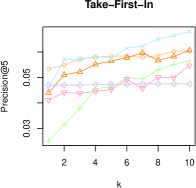
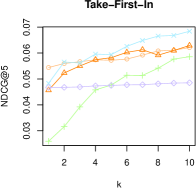
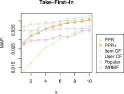
Firstly, the result plots are less smooth than the corresponding plots for the TakeKIn experiments as the additional smoothing induced by repeated randomization is missing. Secondly, the relative assessment of UCF, ICF, MP, RND and WRMF is consistent with those of the randomized TakeKIn experimentation. Most interestingly, $\mathop{P\!P\!R}$ performs better for all $k$ than $\mathop{P\!P\!R\!+}$ (in contrast to the results of the TakeKIn experimentation). This, on the one hand, shows, that the order of input does indeed matter. The worse assessment of $\mathop{P\!P\!R\!+}$ in the chronological order hints at the impact of global frequencies (i. e., popularity of names), as by construction, $\mathop{P\!P\!R\!+}$ increases personalization by reducing the influence of global frequencies. The results in Figure 6 indicate, that the first entered names tend to be more popular names and later a name is entered, the more specific the name is for the user. To underpin this assumption, we calculated for each name its popularity rank, that is, its position within the list of names which is decreasingly ordered by search frequency. We than calculated for each chronological position $p$ the average popularity rank of all names which were search by some user at position $p$ within the user’s search history. Figure 7 shows a positive correlation between the position in the user’s search history and the popularity rank of the corresponding name, indeed indicating that users tend to search first for popular names.

Figure 7: Average popularity rank for all entered names relative to the corresponding position within the users’ search history, indicating that users tend to search first for popular names. To rule out statistical effects, we shuffled the user’s search history and, depicting the corresponding results in Grey.

For reference we also summarize the prediction accuracy of the different recommendation systems for the LeaveLastOut protocol, which uses as much of the chronologically ordered names from the users search history for predicting the remaining (last) names in Table 7. The indicated performance scores support observed the tendencies in the preceding TakeFirstIn experiment.

Table 7: Leave-Last-Out evaluation for all considered recommendation systems.

	Precision@5	Recall@5	NDCG@5	MAP
PPR	0.050	0.031	0.049	0.037
PPR+	0.052	0.031	0.053	0.038
User CF	0.056	0.034	0.055	0.038
Item CF	0.049	0.027	0.051	0.034
MostPopular	0.041	0.025	0.041	0.032
WRMF	0.047	0.028		0.032
Random	0.000	0.000	0.000	0.001

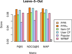
For further supporting the observed characterizations of the different recommendation systems with respect to prediction accuracy, we applied the same evaluation protocol to the set $\emph{Favorite}(u)$ names per user $u$. As the corresponding evaluation data is much more sparse then the set Enter (u) of entered names, we only show the results for the LeaveKOut protocol with $k=5$ and considering only users with at least eight favorite names (resulting in 230 cases). Figure 8 shows the corresponding results for Precision@5, NDCG@5 and MAP for all considered recommendation system respectively. The overall relative assessment of the different system is consistent with the results obtained on the set of entered names - only that $\mathop{P\!P\!R\!+}$ is now even outperforming UCF significantly ($p=0.0362$).

Figure 8: Average performance metrics for the favorite names (Leave-5-Out with 25 repetitions and minimal number of favorite names per user is 8).

3.7 Discussion

In this section we presented results of an experimental setup which aims at assessing the prediction accuracy of different recommendation systems. Beside establishing baseline results for reference, the presented evaluation guides the decision process of choosing a recommendation system for integration in a running application like Nameling.

Considering just the prediction accuracy, the standard preferential PageRank consistently shows best performance for users for which only one or two names are known. In any other case, the user based collaborative filtering approach outperforms all other systems. As it is important to generate good recommendations as soon as possible to catch the user’s interest, it is worth to combine these approaches, recommending popular names to new users, $\mathop{P\!P\!R}$ based recommendations for users with a small search history and UCF otherwise.

But beside prediction accuracy, among others, run time efficiency is an important issue for recommendation systems. In the context of tag recommendation systems it was observed that, in a live setting, many systems fail to provide recommendations within a justifiable time limit [17]. Also the handling of new items (i. e., names) and users has to be taken into account. In the case of name recommendations, the set of names is nearly constant over time, while there is a steady stream of new users using the system while there are very few users using the system for a long period of time. This is due to the fact that the need for a given name typically ends after a short time limit.

Considering the run time efficiency, WRMF is a candidate due to the constant time operations with the latent user and item vectors. But also $\mathop{P\!P\!R}$ an $\mathop{P\!P\!R\!+}$ are efficient to implement, as the results are just averaged over the individual query names of the user’s search history. This operation can already be implemented within a database system which only holds the top similar names $\mathop{P\!P\!R\!+}(i)$ and $\mathop{P\!P\!R}(i)$, respectively, for every name $i$. As the set of names is nearly constant in time, good recommendations for new users can be produced on these precomputed vectors.

Considering the results obtained on the chronologically ordered search history of users, $\mathop{P\!P\!R}$ yields results as least as good as $\mathop{P\!P\!R\!+}$, as depicted in Figure 6. But the results obtained on randomized samples of the user’s search history show significant better performance of $\mathop{P\!P\!R\!+}$. The observations in Section 3.6 indicate that the difference in the prediction accuracy of $\mathop{P\!P\!R}$ and $\mathop{P\!P\!R\!+}$ between the chronological and randomized evaluation can be explained with the tendency that users tend to search first for popular names and later more special names. But this search habits might change with the availability of good recommendation systems. An important reason for the popularity correlated search order is due to the fact, that popular names are more known and a user first thinks of popular names while browsing the system for more suitable names. A good recommendation system will help the user in accessing suitable (i. e., personalized) names more directly.

Summing up, our adaption $\mathop{P\!P\!R\!+}$ of the preferential PageRank is the most promising candidate for implementation in a running application. The choice of $\mathop{P\!P\!R\!+}$ is even more supported by considering the actual favorite names in Nameling, where it even significantly outperforms UCF ($p=0.04$).

4 Diversification of PageRank based Recommendations

The apparent diversity-accuracy dilemma of recommender systems is especially relevant for the task of recommending names, as future parents are often interested in names they like, but which should not be too common within their environment. Concerning prediction accuracy, the simple recommender which constantly recommends only the popular names, already yields reasonable results (cf. 3.6), but is useless for the parent’s need to discover names which are suitable for their children but are yet unknown to them.

So far, we only considered the prediction accuracy for assessing the quality of the different recommendation approaches. This section aims at comparing the recommendation systems with respect to the diversity of the obtained recommendations. For this, we firstly fix our notion of diversity and corresponding evaluation measures and subsequently use these measures for comparing the diversity of the most promising recommendation approaches from Section 3.6.

Finally, we consider different ways for increasing diversity of our $\mathop{P\!P\!R\!+}$ approach by incorporating background information based on networks of given names obtained from Wikipedia, Twitter and Nameling.

4.1 Asessment of Diversity

Diversity of a set of recommended items can either be assessed relative to semantic properties (such as gender or cultural context in the case of given names) or relative to its adaptation to the user’s personal taste (i. e., how diverse recommendations for different users are).

We focus on the aspect of adaptation, because we distinguish between the task of ranking and recommendation in the context of our work, at which the former targets the use case of searching and browsing for given names and accordingly benefits in particular from semantical result diversification, whereas the latter targets the use case of providing a small set of suitable names which adopts primarily to the user’s personal taste.

Assuming diversity of the user’s personal taste, personalization of a given recommendation system Rec can be assessed by measuring the inter-user diversity for different users $u$ and $v$. Accordingly, we consider the personalization index $h$, proposed in [43] $h(u,v)\mathrel{\mathop{:}}=1-\frac{\text{Rec}^{k}(u)\cap\text{Rec}^{k}(v)}{k}.$, where $\text{Rec}^{k}(u)$ denotes Rec’s top $k$ recommended items for user $u$. Identical results for $u$ and $v$ thus yield a value of $h(u,v)=0$ whereas completely different recommendations yield a value of $h(u,v)=1$. The overall personalization performance $h(\text{Rec})$ is assessed by averaging over all pairs of users.

For assessing the prediction accuracy, we focus on the precision scores. Please note that in this section, the impact of varying number of known names on the prediction performance is not in the center of interest and therefore precision scores are calculated for each user on all but the known training items. Accordingly, the precision scores decrease with increasing number of known names, as at the same time the size of the corresponding test sets decreases.

Fig. 9 shows personalization and precision scores for the most promising recommendation systems from Sec. 3.6, namely user based collaborative filtering, weighted matrix factorization, $\mathop{P\!P\!R}$ and $\mathop{P\!P\!R\!+}$.

(a)

(b)

Figure 9: Personalization as measure for assessing diversity and precision applied to the most promising recommendation systems from Sec. 3.5.

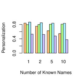
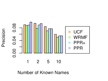
For user based collaborative filtering and $\mathop{P\!P\!R}$, the personalization scores indicate the lowest diversity of the recommendation results, where the scores decrease with increasing number of known names. In contrast, the results obtained from WRMF and $\mathop{P\!P\!R\!+}$ are at a respective constant level for the varying number of known names, at which $\mathop{P\!P\!R\!+}$ achieves the highest scores. The low personalization score for $\mathop{P\!P\!R}$ can be explained with the dominance of global frequencies, i. e., popular names.

4.2 Multi-Graph Aggregation for Increased Diversity

With respect to prediction accuracy and both considered measures for diversity, our $\mathop{P\!P\!R\!+}$ approach already shows an superior trade-off compared to the other considered recommendation systems. Nevertheless, especially in the context of given names, diversity of recommendation results is important, as future parents are using such a system in order to find names which they like, but weren’t aware of so far.

In the following we present and compare different approaches for increasing the diversity of $\mathop{P\!P\!R\!+}$. The evaluation of diversity in an offline setting is very limited, as uncommon items (i. e., names with an high self-information score) are unlikely to be contained in an user’s test set. Also, diversity by itself can be maximized by randomization, but at the same time, the results will show very low accuracy with respect to the user’s personal taste.

We therefore compare the different diversification approaches by considering the trade-off between prediction accuracy (in terms of precision) and diversity (in terms of personalization). All proposed diversification approaches encompass a diversification parameter $\vec{\eta}$, which controls the impact of a second network of given names, intended for introducing diversity to the training data. Formally, we assume a set of graphs $G^{(1)},\ldots,G^{(L)}$ with $G^{(\ell)}\mathrel{\mathop{=}}:(V^{(\ell)},E^{(\ell)})$ over a common vertex set $V\supseteq V^{(\ell)}$ and edge weighting functions $w^{(1)},\ldots,w^{(L)}$ for $\ell=1,\ldots,L$.

Weighted Average

As a baseline approach for combining ranking results obtained from different networks, we consider the weighted average ranking AveRank, which is for given query items $\mathcal{I}\subseteq V$ defined by $\text{AveRank}(\mathcal{I})\mathrel{\mathop{:}}=\frac{1}{L}\sum_{i=1}^{L}\eta_{i}\mathop{P\!P\!R\!+}(\mathcal{I})$ with $\eta_{i}\in[0,1]$ and $\sum_{i=1}^{L}\eta_{i}=1$.

We now look for ways of combining the graphs by themselves in order to benefit from mutual reinforcement of important nodes during the convergence process of the $\mathop{P\!P\!R\!+}$ algorithm. Various ways for combining different graphs exist, of which we consider the following two.

Conditional Multigraph PageRank

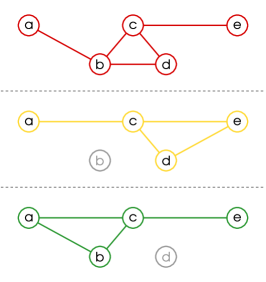
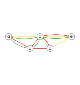
The conditional multigraph PageRank is based on the idea of a multigraph built from $G^{(1)},\ldots,G^{(L)}$ in which edges are additionally labeled corresponding the graph they originated from. Accordingly, multiple edges among vertex pairs may exist, as depicted in Fig. 10b. Applying the intuition of the random surfer model , the basic idea of the conditional multigraph PageRank is, that a random surfer, reaching node $u$ via a certain edge type, will more likely leave $u$ using an edge of the same type, but may nevertheless leave $u$ using any other incident edge. Thus, the importance of each graph’s neighborhood is accented, but nevertheless, interrelations with other nodes as induced by other graphs are also considered. Furthermore, the transition probability of an edge $(u,v)$ scales with the number of graphs containing it. By introducing according stochastic damping factors $(\boldsymbol{\eta})_{\ell_{1},\ell_{2}}\in[0,1]^{L\times L}$, the overall inter-graph transition probabilities can be controlled.

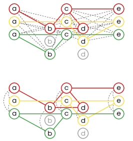
In order to apply standard PageRank calculations, we build a combined (non-multi) graph $\widetilde{G}=(\widetilde{V},\widetilde{E})$, which incorporates the conditional multi-graph approach by construction. For this, we firstly duplicate each node $v\in V$ according to the number of graphs, i. e., $\widetilde{V}\mathrel{\mathop{:}}={v^{1}_{1},\ldots,v^{1}_{n},\ldots,v^{L}_{1},\ldots,v^{L}_{n}}$. Secondly, we include each graph $G_{\ell}$’s connectivity within $\widetilde{E}_{\ell,\ell}$, resulting in $\widetilde{E}_{\ell,\ell}\mathrel{\mathop{:}}=\{(u^{\ell},v^{\ell})\in\widetilde{V}\times\widetilde{V}\mid(u,v)\in E_{\ell}\}$. Finally, for $\ell_{1}\neq\ell_{2}$, we set $\widetilde{E}_{\ell_{1},\ell_{2}}\mathrel{\mathop{:}}=\{(u^{\ell_{1}},v^{\ell_{2}})\mid(u^{\ell_{2}},v^{\ell_{2}})\in E_{\ell_{2}}\}$ and $\widetilde{E}\mathrel{\mathop{:}}=\bigcup\limits_{\ell_{1},\ell_{2}}\widetilde{E}_{\ell_{1},\ell_{2}}$. Edge weights are given by the combined weighting function $\widetilde{w}(u^{\ell_{1}},v^{\ell_{2}})\mathrel{\mathop{:}}=w_{\ell_{2}}(u^{\ell_{1}},v^{\ell_{2}})$. Accordingly, $\widetilde{G}$’s adjacency matrix $A$ is block-wise structured

$$A=\left(\BMAT[8pt]{c:c:c}{c:c:c}A^{1,1}&\ldots A^{1,L}\\ \vdots\ddots\vdots\\ A^{L,1}\ldots A^{L,L}\right)$$

where each $n\times n$ sub-matrix $A^{\ell,\ell}$ corresponds to graph $\ell$’s adjacency matrix and $A^{\ell_{1},\ell_{2}}$ describes transitions from graph $\ell_{1}$ to graph $\ell_{2}$. For calculating PageRank scores on $\widetilde{G}$, its adjacency matrix $A$ has to be normalized in order to be column-stochastic, i. e., all columns sum up to one. The accentuation of inner-graph connectivity is realized by introducing damping factors $\eta_{\ell_{1},\ell_{2}}$ on the graph normalization, such that each of $A^{\ell_{1},\ell_{2}}$’s columns sums up to $\eta_{\ell_{1},\ell_{2}}$. For obtaining the conditional multigraph PageRank score for a given $\mathcal{I}$, we calculate $\text{MultiRank}(\mathcal{I})\mathrel{\mathop{:}}=\mathop{P\!P\!R\!+}(\mathcal{I})$ on $\widetilde{G}$.

Parallel PageRank

A simpler combination of $G^{(1)},\ldots,G^{(L)}$ can be achieved, by interconnecting each node $v\in V$ across all graphs. Fixing the notation introduced for the conditional multigraph PageRank, we build an according graph $\widetilde{G}=(\widetilde{V},\widetilde{E})$ by altering only the inter-graph connectivity to $\widetilde{E}_{\ell_{1},\ell_{2}}\mathrel{\mathop{:}}=\{(u^{\ell_{1}},u^{\ell_{2}})\mid u\in V\}$. For obtaining the parallel multigraph PageRank score for a given $\mathcal{I}$, we calculate $\text{PRank}(\mathcal{I})\mathrel{\mathop{:}}=\mathop{P\!P\!R\!+}(\mathcal{I})$ on $\widetilde{G}$.

Weighting

Please note that the prediction performance of $\mathop{P\!P\!R\!+}$ depends on the edge weighting of the input graph. Accordingly, the weights of inter-network edges may be adopted in order to improve one of the evaluation targets (e. g., depending of the incident node’s connectivity). For our evaluation, we set the weight of every such edge $(u^{\ell_{1}},v^{\ell_{2}})$ with $\ell_{1}\neq\ell_{2}$ to one in order to consider the most general case.

(a)

(b)

(c)

Figure 10: Construction for the conditioned multigraph PageRank: Separate graphs (a), the merged multigraph (b) and the combined graphs, where nodes are duplicated according to the number of networks (c). The construction for the conditional multigraph PageRank is shown on top and the for the parallel PageRank on the bottom right.

4.3 Evaluation

For evaluating the different result diversification approaches for $\mathop{P\!P\!R\!+}$, we consider the network of given names obtained from Nameling’s usage data and combine it pairwise with the co-occurrence graph obtained from Wikipedia and respectively Twitter, as well as the shared category graph obtained from Wiktionary and the shared favorite graph from Nameling. We thereby apply the evaluation protocol from Sec. 3.6, except that all but the training names are used for evaluation. For considering the trade-off between prediction accuracy and diversity, we show the obtained results in a precision/diversity scatter plot. For reference, we also calculated the diversity of the considered user profiles by themselves ($h=0.99$, $I=9.62$, calculated on the first ten test items for $k=1,5$).

Fig. 11 shows the accuracy/diversity scatter plots with respect to personalization on all considered pairs of networks. We only show results obtained for the TakeFirstIn protocol with $k=5$. The results only differ in magnitude for varying $k$ but the overall characteristics are unchanged. We note that all considered multigraph approaches introduce varying amounts of diversity and an accordingly differing level of accuracy.

Figure 11: Diversity vs. accuracy scatter plots for all considered multigraph approaches in the co-occurrence network obtained from Twitter (top row), the co-occurrence network obtained from Wikipedia (2nd row), the shared categories network (3rd row) and shared favorite names network (bottom row) for recommendations based on one, five or ten known names in the left, middle and right column respectively.

We firstly consider the personalization/precision trade-off. The weighted average approach shows similar characteristics for all considered networks. Except for the combination with the Twitter based network, both combined multigraph approaches outperform the considered baseline, where PRank shows overall smother transitions and covers broader ranges of the personalization metric. Nevertheless, MultiRank is the only approach which shows increasing tendencies for the precision scores with increasing personalization score. In combination with the Twitter based network, both combined multigraph approaches show inferior performance than the baseline model.

Summing up, we observe differing characteristics for the accuracy/diversity lemma, hinting at a more pronounced dependence of MultiRank on the inter-network correlations. Nevertheless, the results obtained from the different approaches are complementary and ultimately only a live evaluation of the different graph combinations will reveal, which result diversification approach corresponds best to the user’s expectations.

5 Related Work

The present work introduces a new field of application for analyzing relations among named entities and recommendation systems. It is motivated by the work on the search engine “Nameling”, which is presented in [26]. The ranking performance of the structural similarity metrics based on the Wikipedia corpus relative to the actual usage data which accrued in the running system is evaluated in [27, 28]. The considered approaches are based on work in the field of distributional semantics, link prediction and (more generally) vertex similarity in graphs as well as recommendation systems.

Distributional Semantics

The field of distributional semantics relatedness has attracted a lot of attention in literature during the past decades (see [5] for a review). Several statistical measures for assessing the similarity of words are proposed, as for example in [20, 11, 14, 18, 39]. Notably, first approaches for using Wikipedia as a source for discovering relatedness of concepts can be found in [2, 37, 8].

Vertex Similarity & Link Prediction

In the context of social networks, the task of predicting (future) links is especially relevant for online social networks, where social interaction is significantly stimulated by suggesting people as contacts which the user might know. From a methodological point of view, most approaches build on different similarity metrics on pairs of nodes within weighted or unweighted graphs [16, 19, 23, 24]. A good comparative evaluation of different similarity metrics is presented in [21]. The construction of multigraph extensions to the NameRank algorithm for controlled result diversification are based on [35], where random walks are used to combine the information of different networks.

Recommender Systems

Recommending given names is just a special case for the item recommendation task which is extensively discussed for various fields of application, such as movies [10], tags [15] and products [22]. Notably the characteristics of deriving recommendations from activity logs (rather than explicit user feedback) are discussed in [13] where the uncertainty of implicit feedback taken into account, by attaching an adequate level of confidence to an implicitly expressed interest in an item (e. g., by clicking on the description of a given name). A very good introduction and summary of the evaluation of recommendation systems can be found in [36].

References

- [1] S. Brin and L. Page. The anatomy of a large-scale hypertextual web search engine. In Computer Networks and ISDN Systems, pages 107–117, 1998.
- [2] R. Bunescu and M. Pasca. Using encyclopedic knowledge for named entity disambiguation. In Proc. of EACL, volume 6, pages 9–16, 2006.
- [3] C. Butts. Social network analysis: A methodological introduction. Asian J. of Soc. Psychology, 11(1):13–41, 2008.
- [4] C. T. Butts and K. M. Carley. Some simple algorithms for structural comparison. Comput. Math. Organ. Theory, 11:291–305, December 2005.
- [5] T. Cohen and D. Widdows. Empirical distributional semantics: methods and biomedical applications. J Biomed Inform, 42(2):390–405, Apr. 2009.
- [6] J. Demšar. Statistical comparisons of classifiers over multiple data sets. The Journal of Machine Learning Research, 7:1–30, 2006.
- [7] T. Dunning. Accurate methods for the statistics of surprise and coincidence. COMPUTATIONAL LINGUISTICS, 19(1):61–74, 1993.
- [8] E. Gabrilovich and S. Markovitch. Computing semantic relatedness using wikipedia-based explicit semantic analysis. In Proc. of the 20th int. joint conference on artificial intelligence, volume 6, page 12. Morgan Kaufmann Publishers Inc., 2007.
- [9] Z. Gantner, S. Rendle, C. Freudenthaler, and L. Schmidt-Thieme. Mymedialite: A free recommender system library. In Proceedings of the fifth ACM conference on Recommender systems, pages 305–308. ACM, 2011.
- [10] J. Golbeck and J. Hendler. Filmtrust: Movie recommendations using trust in web-based social networks. In Proceedings of the IEEE Consumer communications and networking conference, volume 96. Citeseer, 2006.
- [11] G. Grefenstette. Finding semantic similarity in raw text: The deese antonyms. In Fall Symposium Series, Working Notes, Probabilistic Approaches to Natural Language, pages 61–65, 1992.
- [12] A. Hotho, R. Jäschke, C. Schmitz, and G. Stumme. Information retrieval in folksonomies: Search and ranking. In Y. Sure and J. Domingue, editors, The Semantic Web: Research and Applications, volume 4011 of Lecture Notes in Computer Science, pages 411–426, Heidelberg, June 2006. Springer.
- [13] Y. Hu, Y. Koren, and C. Volinsky. Collaborative filtering for implicit feedback datasets. In Data Mining, 2008. ICDM’08. Eighth IEEE International Conference on, pages 263–272. IEEE, 2008.
- [14] A. Islam and D. Inkpen. Second order co-occurrence pmi for determining the semantic similarity of words. In Proc. of the Int. Conference on Language Resources and Evaluation (LREC 2006), pages 1033–1038, 2006.
- [15] R. Jäschke, L. Marinho, A. Hotho, L. Schmidt-Thieme, and G. Stumme. Tag recommendations in social bookmarking systems. Ai Communications, 21(4):231–247, 2008.
- [16] G. Jeh and J. Widom. Simrank: a measure of structural-context similarity. In Proc. of the eighth ACM SIGKDD int. conference on Knowledge discovery and data mining, KDD ’02, pages 538–543, New York, NY, USA, 2002. ACM.
- [17] R. Jäschke, F. Eisterlehner, A. Hotho, and G. Stumme. Testing and evaluating tag recommenders in a live system. In RecSys ’09: Proceedings of the third ACM Conference on Recommender Systems, pages 369–372, New York, NY, USA, 2009. ACM.
- [18] T. Landauer and S. Dumais. A solution to plato’s problem: The latent semantic analysis theory of acquisition, induction, and representation of knowledge. Psychological Review, 104(2):211, 1997.
- [19] E. A. Leicht, P. Holme, and M. E. J. Newman. Vertex similarity in networks, 2005. cite arxiv:physics/0510143.
- [20] M. Lesk. Word-word associations in document retrieval systems. American documentation, 20(1):27–38, 1969.
- [21] D. Liben-Nowell and J. Kleinberg. The link-prediction problem for social networks. J. of the American society for inf. science and technology, 58(7):1019–1031, 2007.
- [22] G. Linden, B. Smith, and J. York. Amazon. com recommendations: Item-to-item collaborative filtering. Internet Computing, IEEE, 7(1):76–80, 2003.
- [23] L. Lü, C. Jin, and T. Zhou. Similarity index based on local paths for link prediction of complex networks. Physical Review E, 80(4):046122, 2009.
- [24] L. Lü and T. Zhou. Link prediction in weighted networks: The role of weak ties. EPL (Europhysics Letters), 89:18001, 2010.
- [25] F. Mitzlaff, M. Atzmueller, G. Stumme, and A. Hotho. Semantics of user interaction in social media. In G. Ghoshal, J. Poncela-Casasnovas, and R. Tolksdorf, editors, Proceedings of the 4th Workshop on Complex Networks CompleNet 2013, volume 476 of Studies in Computational Intelligence. Springer, 2013.
- [26] F. Mitzlaff and G. Stumme. Namelings - discover given name relatedness based on data from the social web. In K. Aberer, A. Flache, W. Jager, L. Liu, J. Tang, and C. Guéret, editors, SocInfo, volume 7710 of Lecture Notes in Computer Science, pages 531–534. Springer, 2012.
- [27] F. Mitzlaff and G. Stumme. Ranking given names. In M. Marathe and N. Contractor, editors, Proceedings of the 1st ASE International Conference on Social Informatics, pages 185–191. IEEE computer society, 2012.
- [28] F. Mitzlaff and G. Stumme. Relatedness of given names. Human Journal, 1(4):205–217, 2012.
- [29] F. Mitzlaff and G. Stumme. The power of social co-occurrences. Submitted for Publication, 2013.
- [30] T. Murata and S. Moriyasu. Link prediction of social networks based on weighted proximity measures. In Web Intelligence, IEEE/WIC/ACM Int. Conference on, pages 85–88. IEEE, 2007.
- [31] L. Nelson and J. Simmons. Moniker maladies – when names sabotage success. Psychological Science, 18(12):1106–1112, 2007.
- [32] M. E. J. Newman. The structure and function of complex networks. SIAM Review, 45(2):167–256, 2003.
- [33] S. Rendle, C. Freudenthaler, Z. Gantner, and L. Schmidt-Thieme. Bpr: Bayesian personalized ranking from implicit feedback. In Proceedings of the 25th Conference on Uncertainty in Artificial Intelligence, 2009.
- [34] B. Sarwar, G. Karypis, J. Konstan, and J. Riedl. Item-based collaborative filtering recommendation algorithms. In Proceedings of the 10th international conference on World Wide Web, WWW ’01, pages 285–295, New York, NY, USA, 2001. ACM.
- [35] C. Scholz, M. Atzmueller, A. Barrat, C. Cattuto, and G. Stumme. New insights and methods for predicting face-to-face contacts. Submitted for Publication.
- [36] G. Shani and A. Gunawardana. Evaluating recommendation systems. Recommender Systems Handbook, pages 257–297, 2011.
- [37] M. Strube and S. P. Ponzetto. Wikirelate! computing semantic relatedness using wikipedia. In proc. of the 21st national conference on Artificial intelligence - Volume 2, AAAI’06, pages 1419–1424. AAAI Press, 2006.
- [38] X. Su and T. Khoshgoftaar. A survey of collaborative filtering techniques. Advances in Artificial Intelligence, 2009:4, 2009.
- [39] P. Turney. Mining the web for synonyms: Pmi-ir versus lsa on toefl. In Proc. of the 12th European Conference on Machine Learning, pages 491–502. Springer-Verlag, 2001.
- [40] E. Voorhees and D. Harman. TREC: Experiment and evaluation in information retrieval, volume 63. MIT press Cambridge, 2005.
- [41] M. Weimer, A. Karatzoglou, and A. Smola. Improving maximum margin matrix factorization. Machine Learning, 72(3):263–276, 2008.
- [42] J. Yang and J. Leskovec. Patterns of temporal variation in online media. In Proc. of the fourth ACM int. conference on Web search and data mining, pages 177–186. ACM, 2011.
- [43] T. Zhou, Z. Kuscsik, J. Liu, M. Medo, J. Wakeling, and Y. Zhang. Solving the apparent diversity-accuracy dilemma of recommender systems. Proceedings of the National Academy of Sciences, 107(10):4511–4515, 2010.