Hall A Annual Report
2012

Edited by Seamus Riordan & Cynthia Keppel

1 Introduction

contributed by Cynthia Keppel

The year 2012 marked the end of the 6 GeV era at Jefferson Lab, and the beginning of the next phase in making the 12 GeV upgrade to the Continuous Electron Beam Accelerator Facility a reality. The final months of the 6 GeV scientific program in Hall A facilitated completion of the $g_{2}^{p}$ and $G_{E}^{p}$ experiments. A long process of removing, upgrading and re-installing existing components and systems, and installing new ones, has now begun in preparation for 12 GeV operations, with the expectation to see the first beam back in Hall A in 2014.

The 12 GeV upgrade plans for Hall A, as a subset of the overall laboratory project, are modest, composed largely of requisite beam line upgrades to the beam transport, polarimetry and arc energy measurements. However, the 12 GeV scientific plans for the hall are ambitious, and include multiple new experiment installations such as the Super Bigbite Spectrometer (SBS) program to measure high precision nucleon form factors, the MOLLER experiment to measure the parity-violating asymmetry in electron-electron (Moller) scattering, and the SoLID (Solenoidal Large Intensity Device) program to provide a facility for parity violating and semi-inclusive deep inelastic scattering experiments. In addition to these large-scale efforts, many other compelling experiments will utilize the standard Hall A equipment, some with slight modifications, in conjunction with the higher energy beam.

The last part of the year has been dedicated to preparing for two of the latter, experiments E12-07-108, a measurement of the proton magnetic form factor G${}_{M}^{p}$ [1], and E12-06-114, a measurement of deeply virtual Compton scattering [2], which will be the first experiments to receive beam in the 12 GeV era. It is interesting to note that these first experiments both harken back to the early days of Hall A, where first round experiments then also measured virtual Compton scattering and form factors, albeit at lower Q² and with somewhat different physics foci. It seems perhaps the proverb is true, “The more things change the more they remain the same.” Preparations for E12-07-108 and E12-06-114 have included plans for a largely combined run period, employing both HRS’s, where significant detector upgrades are underway, a hydrogen target, and other complimentary equipment.

This year also brought DOE approval to begin the Super Bigbite Spectrometer (SBS) project. This project consists of a set of three form factor experiments centered around somewhat common equipment and new experimental capabilities. First activities to begin this program include re-design of a magnet from the Brookhaven National Laboratory, pre-research and development of GEM tracking detectors, and a host of scientific development activities including detector construction projects, data acquisition upgrades, and refined physics projections.

Work has continued effectively as well on many other fronts, including infrastructure improvements in data acquisition, offline analysis, and core hall capabilities. Technical preparations have begun for the ³H target experiments anticipated for 2015. Ideas to improve and upgrade also the polarized ³He target, required for instance for the measurement of A${}^{n}_{1}$, are being implemented. Efforts continue also for 2015 and beyond planned experiments such as PREX-II, and APEX. Moreover, there has been active engagement in analyses of past experiments. Here, ten new publications related to Hall A experiments were authored by members of the Hall A collaboration, and seven new Hall A related doctoral theses were successfully defended.

In all, this has been a year of transition - for the laboratory, for Hall A, and also for me as the new Hall Leader. It is an exciting challenge to facilitate the progression of the characteristically excellent standards established here by the Hall A staff and user community into the 12 GeV era. Please accept my many, many thanks to you all for your shared wisdom, valuable advice, and patient support. I look forward to welcoming the higher energy beam into Hall A with you!

2 General Hall Developments

2.1 Møller Polarimeter

Status of the Hall A Møller Polarimeter

contributed by ¹O. Glamazdin, ²E. Chudakov, ²J. Gomez, ¹R. Pomatsalyuk, ¹V. Vereshchaka, ²J. Zhang

¹National Science Center Kharkov Institute of Physics and Technology, Kharkov 61108, Ukraine

²Thomas Jefferson National Accelerator Facility, Newport News, VA23606, USA .

2.1.1 Introduction

The Hall A Møller polarimeter [1] had been built in 1997. It was successfully used to measure a beam polarization for all Hall A experiments with polarized electron beam.

2.1.2 General description

The Møller scattering events are detected with a magnetic spectrometer (see Fig.1) consisting of a sequence of three quadrupole magnets and a dipole magnet. The electrons scattered in a plane close to the horizontal plane are transported by the quadrupole magnets to the entrance of the dipole which deflects the electrons down, toward the detector. The optics of the spectrometer is optimized in order to maximize the acceptance for pairs scattered at about 90^∘ in CM. The acceptance depends on the beam energy. The typical range for the accepted polar and azimuthal angles in CM is $75^{\circ}<\theta{}_{\mathrm{CM}}<105^{\circ}$ and $-6^{\circ}<\phi{}_{\mathrm{CM}}<6^{\circ}$. The non-scattered electron beam passes through a 4 cm diameter hole in a vertical steel plate 6 cm thick, which is positioned at the central plane of the dipole and provides a magnetic shielding for the beam area. The plate, combined with the magnet’s poles, make two 4 cm wide gaps, which serve as two $\theta{}_{\mathrm{CM}}$ angle collimators for the scattered electrons. Two additional lead collimators restrict the $\phi{}_{\mathrm{CM}}$ angle range. The polarimeter can be used at beam energies from 0.8 to 6 GeV, by setting the appropriate fields in the magnets. The lower limit is defined by a drop of the acceptance at lower energies, while the upper limit depends mainly on the magnetic shielding of the beam area inside the dipole.

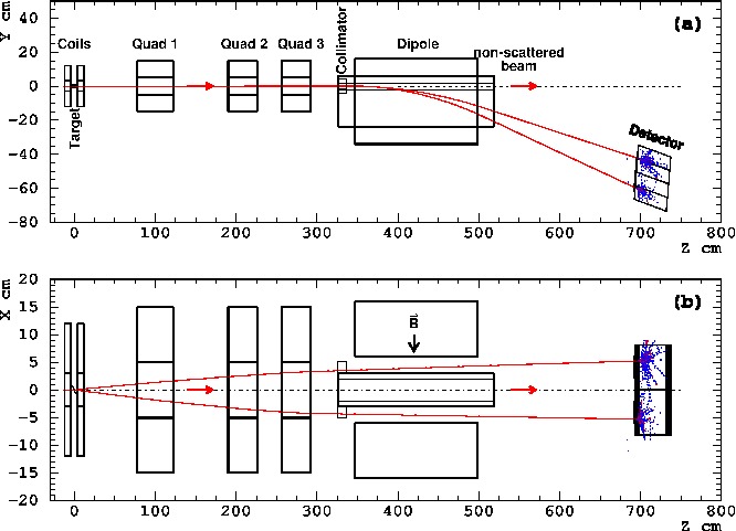
Figure 1: Layout of the Møller polarimeter before 11 GeV upgrade, (a) presents the side view while (b) presents the top view. The trajectories displayed belong to a simulated event of Møller scattering at $\theta{}_{\mathrm{CM}}=80^{\circ}$ and $\phi{}_{\mathrm{CM}}=0^{\circ}$, at a beam energy of 4 GeV.

The detector consists of total absorption calorimeter modules, split into two arms in order to detect two scattered electrons in coincidence. There are two aperture plastic scintillator detectors at the face of the calorimeter. The beam helicity driven asymmetry of the coincidence counting rate (typically about 10⁵ Hz) is used to derive the beam polarization. Additionally to detecting the counting rates, about 300 Hz of “minimum bias” events containing the amplitudes and timings of all the signals involved are recorded with a soft trigger from one of the arms. These data are used for various checks and tuning, and also for studying of the non–Møller background. The estimated background level of the coincidence rate is below 1 %.

2.1.3 12 GeV Upgrade Status

The Hall A Møller polarimeter originally was designed for an electron beam energy range of 1 – 6 GeV. Two factors limit the useful energy range of the polarimeter:

• the spectrometer acceptance, defined by the positions of the magnets and the available field strength, and also the positions and of the collimators;

• the beam deflection in the Møller dipole caused by the residual field in the shielding insertion.

In order to operate the polarimeter at 11 GeV a considerable upgrade of the polarimeter was required. In order to minimize the interference of such an upgrade with the rest of the beam line we did not consider moving the Møller target or the Møller dipole magnet and the Møller detector, as well as replacing the shielding insertion in the dipole magnet.

A few items have to be considered for the higher energy polarimeter design:

1. the positions and settings of the quadrupole magnets;

2. the dipole magnet bending angle;

3. the dipole shielding insertion;

4. the detector position;

5. the beam line downstream of the Møller dipole.

2.1.3.1 Quadrupole magnets position

The acceptance of a Møller polarimeter is defined as the accepted range of the scattering angles in CM, around 90^∘. In Hall A polarimeter a collimator, consisting of two vertical slits between the poles of the dipole magnet and the shielding insertion in the dipole gap plays the most important role in limiting the acceptance. The goal of the quadrupole magnets is to direct the scattered electrons into the slits. With the old (6 GeV) design, two quadrupole magnets ($PATSY$ and $FELICIA$ see Table 1) were used.

GEANT simulation shows that for 11 GeV era power of two and even all three existing Møller quadrupole magnets is not enough. In order to cover the new beam energy range of 0.8 – 11 GeV we proposed to move the first quadrupole 40 cm downstream and to install the fourth quadrupole with its center at 70 cm from the Møller target.

The new quadrupole magnet was designed by Robin Wines. The magnet is shown on Fig. 2. The new quadrupole has been field mapped by Ken Bagget  [2] before installation on the Hall A beam line and the results for the new magnet are presented in Table 1. A new bench was designed and manufactured to install the new quadrupole and to shift the first magnet ($PATSY$). A distance between the Møller target and the new quadrupole magnet center is 0.684 m. A distance between the Møller target and the first Møller quadrupole magnet is 1.334 m. The second and the third Møller quadrupole magnets position is unchanged.

Available $Danfysik$ power supply from Accelerator Division will be used to power the new Møller quadrupole magnet to save money. It is already installed and working, but the EPICS controls have not been done. It is a work in progress.

Table 1: Parameters of the Møller quadrupole magnets.

Møller notation	Q0	Q1	Q2	Q3
MCC notation	$MQO1H01$	$MQM1H02$	$MQO1H03$	$MQO1H03A$
Name	$new$	$PATSY$	$TESSA$	$FELICIA$
Bore, cm	10.16	10.16	10.16	10.16
Effective length, cm	36.58	44.76	35.66	35.66
Maximum current, A	300	300	280	280
Pole tip field at 300 A, kGs	6.39	5.94	6.03	6.14

Figure 2: New quadrupole magnet for Møller polarimeter.

2.1.3.2 Dipole bending angle

The old Møller electrons bending angle in the dipole is 10^∘. A dipole current of about 700 A and a field of about 19.2 kGs is needed to keep this bending angle at 11 GeV. The maximal magnetic field measured in this dipole in Los Alamos was 17.5 kGs. The present dipole power supply provides the maximal current of 550 A. This current is not enough to provide for the beam bending angle in dipole of 10^∘ at the beam energy 11 GeV. This limitation, along with the problem of shielding the beam area at high fields, described below, is mitigated by reducing the bending angle from 10^∘ to 7.0^∘. The smaller bending angle allows to keep the existing Møller dipole and its power supply. The reduction of the bending angle requires a new detector position, as it will be described below.

2.1.3.3 Dipole shielding insertion design

The dipole shielding insertion attenuates the strong dipole magnetic field in the region where the main electron beam passes through the dipole. It was designed for the dipole magnetic field up to 10 kGs. This field is enough to bend the Møller electrons to the Møller detector at a beam energy of 6 GeV. For a higher beam energy and a stronger magnetic field the shielding insertion becomes saturated leading to a strong residual field and a large deflection of the electron beam..

The diameter of the bore in the shielding insertion is 4.0 cm. The diameter of the electron beam line before and after the Møller polarimeter is 2.54 cm. A coaxial magnetically isolated pipe, made of magnetic steel AISI-1010, was placed inside the bore (see Fig. 3) to increase the attenuation of the shielding insertion. The inner pipe diameter is 2.5 cm and the outer diameter is 3.4 cm. The shielding pipe consists of eight assembled together sections to reduce the cost. The shielding pipe is centered in the shielding insertion bore with seven isolating rings made of a non-magnetic aluminum 6061-T6. The total shielding pipe length is 202.4 cm. It is about 15 cm longer than the shielding insertion length in order to reduce the influence of the fringe field outside of the shielding insertion.

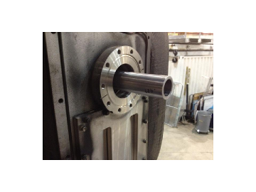
Figure 3: Møller dipole assembly with additional shielding pipe in the shielding insertion.

The new design allows to attenuate to an acceptable level the dipole magnetic field up to 14.8 kGs. A field of 14.0 kGs (and power supply current 513 A) corresponds to the beam energy of 11 GeV and the dipole bending angle 7.0^∘. This field can be provided with the existing power supply.

The TOSCA simulated fields in the dipole gap, in the shielding pipe and the expected electron beam shift on the Hall A target and in the beam dump are shown in Fig. 4. A new vertical corrector is installed downstream of the Møller dipole (see Sec. 2.1.3.5) to compensate the beam shift at high beam energies.

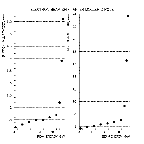
Figure 4: TOSCA result for the Møller dipole with the 10 cm extended shielding pipe. The electron beam shift on the Hall A target (left picture) and in the Hall A beam dump (right picture).

2.1.3.4 Detector position and shielding

Because of the smaller bending angle of the Møller electrons the detector has to lifted by 10cm. The beam line downstream of the dipole also has to be modified. Originally, it was planned to re-use the old detector shielding box with some modifications. It occurred that the design of the old box was in conflict with the design of a new beam line girder downstream of the Møller detector. A new shielding box was designed, manufactured and installed at the new position on the Hall A beam line (see Fig. 5).

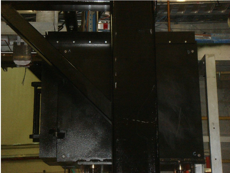
Figure 5: A new Møller detector shielding box on the Hall A beam line.

Before the upgrade the beam pipe diameter after the Møller dipole was 6.35 cm (2.5 inches). The beam pipe diameter over the detector shielding box was 10.16 cm (4 inches), and after that (girder area) 2.54 cm (1 inch). After the upgrade one 6.35 cm (2.5 inches) pipe is used between the Møller detector and the beam line girder.

Lead bricks on the top of the shielding box and and along the beam line downstream of the Møller dipole have been reassembled in accordance with the new beam line design.

2.1.3.5 New girder design downstream of the Møller dipole

Precise knowledge of the beam position and angle on the Møller target is important for the optimal beam tuning and for understanding of the systematic errors of the beam polarization measurements. The old beam line provided only three BPMs for the position/angle measurements:

• BPM $IPM1H01$ - in 1 m upstream of the Møller target;

• BPM $IPM1H04A$ - upstream of the Hall A target (in 17 m downstream of the Møller target);

• BPM $IPM1H04B$ - in the Hall A beam dump.

There were three (at least two) Møller quadrupole magnets, Møller dipole, two quadrupole magnets downstream of the Møller detector and a few beam position correctors between BPM $IPM1H01$ and BPM $IPM1H04A$. Because of that precise information about the beam position and especially beam angle on the Møller target and good beam tuning was not available.

In the new beam line design a new BPM (see Fig. 6) is installed on the girder downstream of the Møller detector. The new BPM is located $\sim{}$7 m downstream of the Møller target. Centering of the beam with the Møller quadrupole magnets and dipole should provide correct beam tuning for the beam polarization measurement and precise information about the beam position and angle on the Møller target.

Figure 6: A new girder downstream of the Møller detector shielding box on the Hall A beam line. From left to right: new vertical corrector $MBD1H04$, focusing quadrupole magnet $MQAH04$ and new beam position monitor $IPM1H04$.

At high energies the shielding insertion in the Møller dipole is saturated and the residual field deflects the beam down (see Fig. 4). A new vertical corrector (see Fig. 6) was installed on the girder to compensate for this effect.

2.1.4 Møller polarized electron targets

Magnetized ferromagnetic materials are used to provide polarized electrons in the target. The average electron polarization in such targets is about 7-8%. It is not theoretically calculable with an accuracy sufficient for polarimetry, and has to be somehow measured. The uncertainty of this value is typically the dominant systematic error of the the Møller polarimetry. Two different techniques to magnetize ferromagnetic targets are used.. The first one - the “low field” technique - uses a thin ferromagnetic foil tilted at a small angle to the beam and magnetized in the foil’s plane by a relatively weak magnetic field ($\sim{}$20 mT) directed along the beam. The second one - the “high field” technique - uses a thin ferromagnetic foil positioned perpendicular to the beam and polarized perpendicular to its plane by a very strong field ($\sim{}$3 T). Description and comparison of both types of the polarized electron targets can be found in  [3]. The Hall A Møller polarimeter is a unique polarimeter which uses both this techniques. This allows a better understanding of the systematic error associated with target polarization.

2.1.4.1 “Low field” polarized electron target status

A detailed description of the “low field” target is done in  [4]. The target was used with the Hall A Møller polarimeter in 2005 - 2009. The target consists of six foils, of Supermendure and iron with different thickness from 6.8 $\mu$m to 29.4 $\mu$m, fixed at an angle of 20.5^∘ to the beam in the $YZ$ plane, magnetized by a $B_{Z}\sim{}0.035$ T field.

The target holder design is shown on Fig. 7. The holder can move the targets across the beam in two projections: transversely - along $X$, and longitudinally - along the longer sides of the foils (a line in the $YZ$-plane, at 20.5^∘ to $Z$). The goal is to study the observed effects of non-uniformity of the target magnetic flux, measured by a small pickup coil at different locations along the foil. Systematic error budget for the Møller polarimeter with the “low field” polarized electron target is presented in Tab. 2

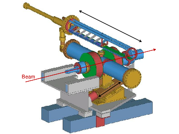
Figure 7: The “low field” target holder design. The electron beam direction and directions of the target motion in two projections are shown.

In the beginning of 2011 after PREX and DVCS experiments the “low field” target was restored back to the Møller polarimeter for the beam polarization measurements for g2p experiment. There were a few reasons to choose the “low field” target for g2p experiment:

• g2p experiment does not require high precision of the beam polarization measurement;

• g2p experiment was running with very low beam current 0.1 $m$A. A maximal efficient thickness of the “high field” target is $\sim{}$10 $\mu$m. A maximal efficient thickness of the “low field” target is $\sim{}$90 $\mu$m. Thus, using of “low field” target allows to reduce essentially time required for the beam polarization measurement with the same statistical error;

• operation of the “low field” target is cheaper because it does not require expensive cryogenics;

• operation of the “high field” target at present requires a daily accesses to the Hall to feed the target superconducting magnet.

The “low field” target was successfully used during the running of the g2p experiment. The “low field” target is installed on the Hall A beam line now and it will be used for the Møller polarimeter commissioning after the 11 GeV upgrade.

2.1.4.2 “High field” polarized electron target status

Experiment PREX required a polarimeter accuracy of $\sim 1\%$. As it is shown in Tab. 2, the Møller polarimeter with the “low field” target can not meet the requirement. Instead, a new “high field” polarized electron target for the Hall A Møller was built. The “high field” technique [5] uses a strong magnetic field - larger than the magnetic field inside of the ferromagnetic domains. The field should orient the magnetization in the domains along the field direction and drive the magnetization into saturation. In the polarimeter, the magnetic field is parallel to the beam direction. The foil is perpendicular to the field, in order to minimize the effects of the magnetization in the foil plane, and is magnetized perpendicular to its plane. The value of the magnetization (and of the average electron polarization) at saturation depends only on the material properties, and for pure iron can be derived from the existing world data [6].

Table 2: Systematic errors for the Hall A Møller polarimeter with the “low field” and the “high field” polarized electron targets.

Variable	“Low field”	“High field”
Target polarization	$1.5\%$	$0.35\%$
Analyzing power	$0.3\%$	$0.3\%$
Levchuk-effect	$0.2\%$	$0.3\%$
Background	$0.3\%$	$0.3\%$
Dead time	$0.3\%$	$0.3\%$
High beam current	$0.2\%$	$0.2\%$
Others	$0.5\%$	$0.5\%$
Total	$1.7\%$	$0.9\%$

Design of the “high field” polarized electron target is shown on Fig. 8. The target consists of:

• a superconducting magnet for a maximal magnetic field of 4 T. The magnet needs liquid He⁴ at low pressure;

• a target holder with a set of four iron foils with the purity of 99.85$\%$ and 99.99$\%$. The foils thicknesses are 1,4,4 and 10 $\mu$m to study possible sources of systematic errors (see Fig. 8);

• a mechanism of target foils orientation along the magnetized field;

• a mechanism for targets motion into the beam;

• a mechanism of the magnetic field orientation along the beam.

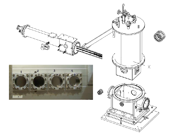
Figure 8: Design of the “high field” polarized electron target. The target holder with four pure iron foils is shown on photo.

The “high field” target was used in 2010 for the beam polarization measurements during the PREX and DVCS experiments running. As it is seen from Tab. 2 using of the “high field” target allows to increase the accuracy of the beam polarization measurements by a factor of two. It should be noted that a successful operation of the “high field” requires considerable efforts:

• improvements of the target foils and magnetized field alignment;

• gaining the target operation experience;

• a systematic error study;

• building a supply line for liquid He⁴.

2.1.5 Møller polarimeter DAQs

The Hall A Møller polarimeter has two DAQs:

• old DAQ based on combination of CAMAC and VME modules;

• new DAQ based on FADC.

The old DAQ is fully operational with both polarized electron targets, well understood but slow, occupies a few crates and uses a few hundred cables to connect modules etc. New DAQ based on FADC is fast, generates two two types of triggers, compact, but not fully operational yet. Running of two different DAQs in parallel and comparison of the results gives a unique opportunity to study possible sources of systematic errors.

2.1.5.1 Old Møller DAQ upgrade status

Present DAQ for the Moller polarimeter detector has been designed in the mid-90th. It uses a lot of slow modules not available in stock anymore. The main goals of the electronics upgrade for the Moller polarimeter are:

• to increase bandwidth (up to 200 MHz) of the detector system;

• to reduce readout time from ADC and TDC modules;

• to replace the old PLU module LeCroy-2365 that is not available in stock anymore.

The list of modules to be replaced:

• to increase bandwidth:

  • PLU module LeCroy-2365, bandwidth $<75$ MHz, CAMAC replaced with PLU module based on CAEN V1495 board (bandwidth 200 MHz, VME);

  • Discriminator   Ortec-TD8000, input rate $<150$ MHz, CAMAC replaced with P/S 706 (300 MHz, NIM), modified for remote threshold setup with DAC type of VMIC4140;

• to reduce readout time:

  • ADC LeCroy 2249A, 12 channels, CAMAC replaced with QDC CAEN V792 (32 channels, VME);

  • TDC LeCroy 2229, CAMAC replaced with TDC V1190B (64 channels, 0.1 ns, VME).

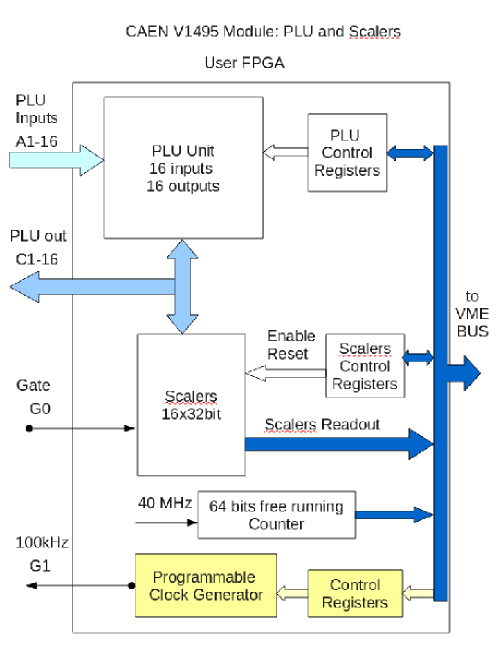
Figure 9: PLU diagram for CAEN V1495 module.

Diagram for new PLU unit based on CAEN V1495 module is shown on Fig. 9. The module CAEN V1495 has the following parameters:

• Input bandwidth $\sim{}$200 MHz;

• 2 input ports x32 bits;

• 1 output port x32 bits;

• 2 input/output front LEMO connectors;

• The FPGA “User” can be reprogrammed by the user using custom logic functions.

Firmware for the PLU module is under development and will consists of the following units:

• Programmable Logical Unit (PLU): 16 inputs, 16 outputs;

• Scalers unit: 16 channels, 32 bit, gate input, connected to PLU outputs;

• Free running 64 bit timer with base frequency 40 MHz.

All the modules required for the upgrade have been procured. The work is in progress. We plan to use the old DAQ after the upgrade at least until the new DAQ based on flash-ADC will be fully operational with both the low and high field targets (see details below in Sec. 2.1.5.2). Also, running of two different DAQs in parallel provides a unique opportunity to study systematic errors.

2.1.5.2 Status of FADC DAQ for the Moller detector

A new DAQ based on the JLab-built FADC was created in 2009 for PREX experiment to be operated with the new high field polarized electron target (see  [7],  [8]). The schematics of the new DAQ is shown on Fig. 10.

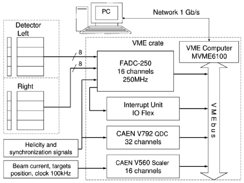
Figure 10: Scheme of a new Møller DAQ based on FADC.

There are some differences between the old and the new DAQ due to differences between the low field and the high field targets operation. For the low field target, the target polarization is a function of the particular foil, the foil coordinate and the magnetic field of the magnetized Helmholtz coils. The direction of the magnetic field is flipped every run to reduce the systematic error. For each run the old DAQ with analyzer is doing the following:

• ramps up the current in the Helmholtz coils;

• reads out the value of the current;

• starts the data taking when the field is established;

• reads out of the foil number and the coordinate of the foil on the beam line;

• reads out of the beam position;

• turns off the current in the Helmholtz coils when the required number of events has been acquired;

• calculates the foil polarization for the particular place of the foil and for the particular magnetizing field and the field direction;

• uses the calculated foil polarization for the beam polarization calculation.

There are two versions of analyzers to run the old DAQ with the low field and the high field targets.

As it was mentioned above, FADC was built to run with the high field target. For this configuration the target is fully saturated and the target polarization is a constant for any foil, foil coordinate and magnetic field. Magnetizing field in the superconducting magnet is turned on in the beginning of the beam polarization measurement and turned off in the end of the measurements. The FADC DAQ does not perform some functions needed for the low field running and, therefore, for the low field running the old DAQ is mandatory while the new DAQ is optional.

The DAQ based on the FADC generates two types of triggers:

1. helicity flipping triggers (integral mode / scalers);

2. data triggers (single events).

There is a good agreement between the old and the new DAQs in scalers mode (see Fig. 11.)

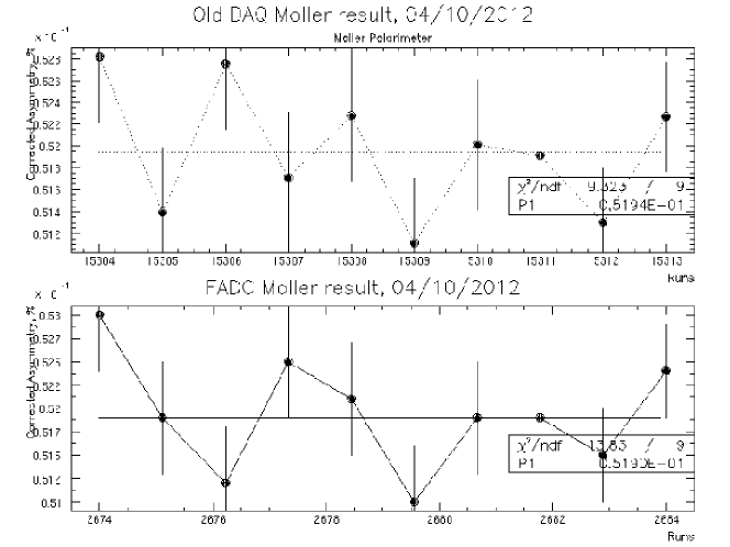
Figure 11: Comparison of results of the beam polarization measurements with the old and the new Møller DAQs in the scaler mode.

Running of the FADC in the data trigger mode is important to study the systematic errors. The triggers data should help to:

• improve the GEANT model of the polarimeter;

• increase the accuracy of the evaluation of the average analyzing power;

• study the Levchuk-effect.

At the moment, the work on the event data analysis is in progress.

2.1.6 Summary

The beamline part of the Møller polarimeter 11 GeV upgrade is completed. The polarimeter can be operated in the beam energy range of 0.8 - 11.0 GeV. The Møller polarimeter is ready for commissioning with the beam. The remaining work includes modifications and checkout of the DAQ system, the “high field” target, a cryogenics line to feed the “high field” magnet, and the documentation for the Møller polarimeter operations after upgrade.

2.2 Compton Polarimeter

The Compton Polarimeter Upgrade

contributed by Sirish Nanda.

2.2.1 Overview

The Hall A Compton Polarimeter provides electron beam polarization measurements in a continuous and non-intrusive manner using Compton scattering of polarized electrons from polarized photons. A schematic layout of the Compton polarimeter is shown in Fig.12. The electron beam is transported through a vertical magnetic chicane consisting of four dipole magnets. A high-finesse Fabry-Perot (FP) cavity located at the lower straight section of the chicane with the cavity axis at an angle of 24 mrad with respect to the electron beam, serves as the photon target. The electron beam interacts with the photons trapped in the FP cavity at the Compton Interaction Point (CIP) located at the center of the cavity. The Compton back-scattered photons are detected in an electromagnetic calorimeter. The recoil electrons, dispersed from the primary beam by the third dipole of the chicane are detected in a silicon micro-strip detector. The electron beam polarization is deduced from the counting rate asymmetries of the detected particles. The electron and the photon arms provide redundant measurement of the electron beam polarization.

In the recent years the Compton polarimeter has undergone a major upgrade[1] to green optics, in order to improve accuracy of polarimetry for high precision parity violating experiments at lower energies such as PReX[3]. The conceptual design of the green upgrade utilizes much of the the existing infrastructure of the present Compton polarimeter. The original Saclay built 1064 nm FP cavity has been replaced with a high power 532 nm system. In addition, the electron detector, photon calorimeter, and data acquisition system have been upgraded to achieve beam polarimetry accuracy of 1% at  1 GeV beam energy. The new systems have been operating successfully in Hall A beam line with about 3 kW of cavity power for the past two years. Electron beam polarimetry was carried out successfully during the PReX experiment with the upgraded polarimeter. Preliminary results indicate  1.5% accuracy in the electron beam polarization has been achieved. Recently, the cavity power has been boosted to over 10kW with new low loss mirrors. The higher power cavity was successfully commissioned with beam during the g2p experiment in 2012.

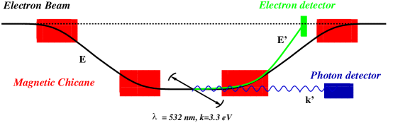
Figure 12: Schematic layout of the Hall A Compton polarimeter.

Additionally, as part of the CEBAF 12 GeV upgrade, the Hall A Compton polarimeter is being upgraded[4] to accommodate 11 GeV beam envisioned for Hall A. The construction of the 12 GeV upgrade is proceeding well with expected completion in 2013 and commissioning with beam in early 2014. At higher energies in the 12 GeV era, Compton polarimetry with 1064 nm infrared light has sufficient analyzing power to be an attractive option that provides higher photon density with less complications. Preliminary investigation into a high power infrared cavity has been started at the Compton polarimetry laboratory. Similarly, development of a high speed data acquisition system to keep pace with the higher luminosities of the upgraded polarimeter has been started as well. Discussions on designs for new electron and photon detectors optimized for the 12 GeV era, are in preliminary stages.

2.2.2 Fabry-Perot Cavity

The newly installed optics replaces the original infrared cavity with a high gain 532 nm green cavity capable of delivering 3 kW of intra-cavity power. Recent advances in the manufacturing of high reflectivity and low loss dielectric mirrors as well as availability of narrow line width green lasers facilitates the feasibility of our challenging design goal. High gain cavities at 532 nm have been successfully constructed by the PVLAS[5] group with geometry and gain comparable to our proposed design. A schematic layout of the optical setup for the upgrade is shown in Fig. 13.

Our solution for the green laser system begins with a narrow line CW fiber coupled Nd:YAG seed laser operating at 1064 nm (Innolight Mephisto S [6]). The beam from the seed laser is then amplified by a Ytterbium doped fiber amplifier (IPG Photonics[7]) which can produce up to 10 W of CW beam while maintaining the line-width and the tunability of the seed laser. The amplified infrared beam is then shaped with lenses L_a and L_b to pump a Periodically Poled Lithium Niobate (PPLN) crystal supplied by HC Photonics [8]. The PPLN crystal is placed in a temperature controlled housing equipped with a thermo-electric heat pump to maintain the temperature of the PPLN crystal at about 60^o with better than .05^o regulation. This temperature corresponds to the quasi-phase matching condition for the PPLN necessary to generate the second harmonic of the pump beam at 532 nm. Typically about 2 W of 532 nm beam is generated with about 5 W of 1064 nm pump beam.

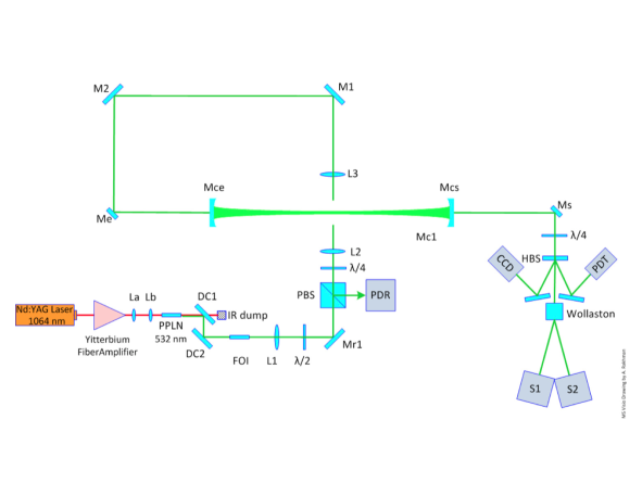
Figure 13: Optical setup of the green Compton polarimeter.

The green beam from the PPLN laser is then separated from the infrared pump with a pair of dichroic mirrors (DC1 and DC2), and transported through polarization conditioning optics and mode-matching lenses (L₁ - L₃) to produce circularly polarized light with the same Gaussian beam profile as the TEM₀₀ mode of the FP cavity. The beam is then injected to the 850 mm long cavity using conventional beam steering optics to properly couple the beam to the cavity. The cavity, constructed out of Invar, has dielectric mirrors mounted on adjustable gimbaled mounts with special ports for the transport of the electron beam. The structure, held in ultra-high vacuum, is part of the electron beam line in Hall A.

Part of the laser beam reflected from the cavity is steered by a polarizing beam splitter to a photo-diode receiver PDR. The PDR signal is used to lock the cavity on resonance using the well known Pound-Drever-Hall locking scheme. The part of the laser beam transmitted through the cavity is converted back to linearly polarized light and analyzed in a Wollaston polarimeter. The intensities of the analyzed horizontal and vertical polarization components of the beam are measured in integrating spheres S₁ and S₂. In addition, a small part of the transmitted beam, separated with a holographic beam splitter, is used for beam monitoring instruments.

The green laser systems and FP cavity have been in development in the Compton Lab for the past few years with participation from many graduate students from collaborating institutions. The development work was successful in late 2009 with stable lock acquisition with dielectric mirrors supplied by Advanced Thin Films[9] (ATF) and homemade locking electronics. The system was then installed and commissioned in the Hall A beam line in early 2010 in preparation for the PReX experiment. During the commissioning, calibration of the laser beam power and polarization transfer functions were carried out in order to accurately determine the power and polarization of the light trapped inside the cavity.

As reported in last year’s annual report, this cavity power saw a major boost in power in 2011 in preparation for the g2p experiment with 1$\mu$A beam current. In early 2012, taking advantage of schedule delays of the experiment, the green cavity was dismantled again and the cavity mirrors were changed to new set of mirrors supplied by ATF. During this down time, the PPLN setup was realigned to restore its conversion efficiency. The power and polarization transfer functions were measured again. With the entire system retuned, lock was acquired in the cavity with the new mirrors at 10 kW, far exceeding our expectation. Shown in Fig. 14 are strip-charts of various cavity parameters as a function of time during this lock acquisition. The blue line shows the power in the cavity whereas the orange line shows the power reflected by the cavity, both making a sharp transitions upon lock acquisition. For the 10 kW performance, the infrared laser was set at 5 mW to seed the fiber amplifier which produced 4 W of 1064 nm light to pump the the PPLN subsystem resulting in 1 W of 532 nm green light. With 20% transport losses, only 0.8 W of the green light was injected into the cavity. The cavity gain was about 1.2$\times$10⁴ resulting in intra-cavity power of 10 kW.

Following the successful running of the FP cavity during the g2p experiment, at the beginning of the long shutdown of CEBAF in June 2012, the cavity performance was further improved before preparing the optics table for the 12 GeV upgrade. Optics data for the final setup were recorded. Preliminary results have indicated that more power is possible before instabilities set in. These data are under analysis.

Figure 14: Stable lock acquisition with 10 kW intra-cavity power in the green cavity. The The blue line shows the power in the cavity making a transition from 10 kW locked state to zero in unlocked state. The orange line show the corresponding power reflected by the cavity.

Test setup in the Compton Lab is being established in order to continue further development work on laser systems and FP cavities. In particular, the optical setup in the Compton lab is being modified to handle both 1064 nm infrared and 532 nm green beams with minimal setup changes. In the 12GeV era of CEBAF, the infrared system becomes competitive since the cavity power in the infrared is generally significantly higher than that in the green, while the analyzing power remains adequate. The old Saclay cavity has been set up in the Compton Lab to provide a platform cavity development. The cavity ends have been modified with new mirror mounts to accommodate the smaller ATF mirrors while providing adjustment of their angular alignment. With the new mechanism the mirrors can be manually aligned with respect to the cavity axis prior to establishing vacuum in the cavity. Preliminary results indicate the alignment concept works well. Successful establishment of fundamental TEM₀₀ resonant mode under vacuum was achieved in 2012. Locking exercises are yet to be performed.

2.2.3 Detectors

The photon detector, a Carnegie Mellon University (CMU) responsibility, consists of a single GSO crystal, 60 mm in diameter and 150 mm in length, fabricated by Hitachi Chemicals Ltd. This detector was removed from Hall A setup for tests in Hall C in 2011. It was successfully reinstalled in Hall A in early 2012 with help from M. Friend and A. Camsonne for the g2p test run. As illustrated in Fig. 15 during the g2p experiment, the GSO calorimeter obtained a high quality Compton scattering spectrum with the 10 kW cavity. Better than 100 signal-to-background ratio was obtained with minimal effort in beam tuning. Observed counting rates were in accordance with a 10 kW of stored photon power confirming the power in the cavity previously calculated with optical measurements.

For higher photon energies in the 12 GeV era, a single crystal PbWO₄ calorimeter is under study. With high density of 8.3 g/cc, PbWO₄ offering 0.9 cm radiation length and 2.2 cm Moliere radius, could be an ideal solution for a compact calorimeter. GEANT simulation are being carried out by Franklin et al. at CMU to study applicability of this material for the 12GeV Compton polarimeter and determine optimum geometry. Discussions are being held with the Shanghai Institute of Ceramics[11] for the feasibility of fabricating large diameter PbWO₄ cylindrical single crystal.

The present data acquisition system has the capability to count photons and electrons up to 100 kHz rate at 30 Hz electron beam spin-flip rate. With the higher luminosity of the new cavity and higher spin-flip rates offered by the CEBAF polarized electron source, higher counting rate capabilities are required. This long standing necessity to upgrade the counting data acquisition system to 1 MHz counting rate at 1 kHz spin flip rate has been under taken by Michaels et al.. Recent bench tests of a prototype system with a pulser signal show that more than 1 MHz rate will be achievable.

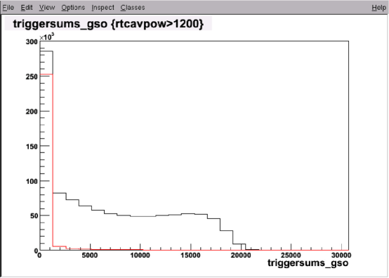
Figure 15: The first Compton scattering spectrum obtained with the GSO calorimeter with the 10 kW cavity. The black solid line, obtained with laser on, is the counting rate as a function of photon energy showing a sharp Compton edge corresponding to back scattered photons. The solid red line is with laser off showing the background rate.

The electron detector supplied by Laboratoire de Physique Corpusculaire IN2P3 Universite Blaise Pascal, Clermont-Ferrand has 4 planes of 192 silicon micro-strip of 0.5 mm thickness with 240 $\mu m$ pitch. The expected resolution is about 100 $\mu m$. A high precision vertical motion of 120 mm for the detector has been incorporated to the design so as to facilitate covering the recoil electrons corresponding to the Compton edge over a broad range of energies. The electron detector along with its associated mechanical structures and electronics were installed Although Compton scattering spectra and asymmetry were successfully obtained with 3 GeV electron beam and the old 1064 nm FP cavity. However, the detection efficiency of the micro-strips was found to be unacceptable, at about 10-20%, due to poor signal-to-noise ratio. The detector was removed from the beam-line and sent back to Clermont-Ferrand to study the signal-to-noise characteristics of the micro-strips with a cosmic tray test setup. A 1 mm thick Si micro-strip detector was procured from Canberra systems to study its signal compared to the 0.5 mm micro-strips in the cosmic tests.

The Clermont-Ferrand team Joly et al.[10] concluded their cosmic studies in early 2012. As expected the thicker Si yielded twice the signal of the thinner ones. In principle, either detector should perform with good efficiency if noise levels, electronics or electron beam related, in Hall A environment is less than 7 mV. With higher noise levels where one has to set the detection thresholds higher, as illustrated in Fig. 16, the thin strips lose efficiency rapidly with increasing thresholds while the 1 mm thick detector retain higher efficiency till about 14 mV. The electron detector was re-installed in Hall A in early 2012 for the g2p test run. However, we ran out of beam time before conclusive beam tests could be made. During the long shutdown of CEBAF, cosmic tests are planned in Hall A. Furthermore, discussions are under way with University of Idaho for possible beam tests with a low energy electron machine at Idaho.

Ideally, a redesign of the front end electronics is necessary to yield acceptable signal-to-noise ratios. With declining support from Clermont-Ferrand University for the electron detector, a new front end is unlikely. Discussions are under way with University of Manitoba and Mississippi State University to address the electron detector issues in the 12 GeV era. In the interim, the thick silicon micro-strips remain as the viable option for the electron detector subject to successful beam tests.

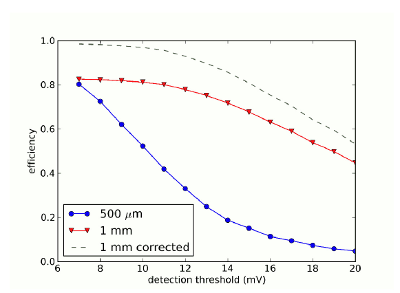
Figure 16: Threshold scan of detection efficiency for the 0.5 mm thick (blue) and 1 mm thick (red)Si micro-strip detectors with cosmic rays. The solid red curve is for the 1 mm Si strips where as the solid blue is for 0.5 mm thick Si. The dashed curve is for the actual efficiency of 1 mm Si corrected for mis-positioning in the experiment

2.2.4 The 12 GeV Upgrade

The Hall A Compton Polarimeter is being upgraded to 11 GeV as part of the CEBAF 12 GeV upgrade project. Before the upgrade, the dipole magnets, the main transport elements of the electron beam line chicane, were configured to produce a 300 mm vertical displacement at 1.5 T for 8 GeV electron beam. In order to minimize cost, the conceptual design of the 12 GeV upgrade simply reuses the same magnets with a reduced bend angle to produce a 218 mm chicane displacement. In the final design, this displacement has been further reduced to 215 mm. Shown in Fig. 17 is a computer model of the Compton polarimeter beam line before and after the upgrade. As shown in the figure, the 2nd and the 3rd dipole magnets, the optics table, and the photon detectors will be raised up by 85 mm. The scope of the upgrade (WBS 1.4.1.5.2) consists of reconfiguration the electron beam chicane, changes to the optical setup, electron and photon detectors to be compatible with 11 GeV configuration. Additionally, the section of the beam pipes between the 3rd and the 4th dipoles is being enlarged substantially to accommodate the larger acceptance of the scattered electrons with a green FP cavity.

Figure 17: Model of the 12 GeV Compton polarimeter in Hall A Beam line before and after the upgrade. Shown in blue are the dipole magnets of the chicane. The two middle dipoles, the optics table, and the photon detector are being raised by 85 mm for the 12GeV Upgrade

With higher energy, synchrotron radiation in the Compton chicane increases dramatically both in flux and hardness. Simulation by Quinn et al. show that at 11 GeV with 100 $\mu$A beam, energy deposited from synchrotron radiation will be about 10-20% of that from Compton scattered electrons from a 10kW green cavity. This poses a major dilution of asymmetry for the integrating photon detector. However, TOSCA simulation by Benesch shows that addition of passive iron plates in the fringe field region of the dipole magnets will reduce the magnetic field seen by the photon detector by an order of magnitude, thus reducing synchrotron radiation background to negligible level. Shown in Fig. 18 is a schematic representation of the synchrotron radiation background and its suppression scheme. Dipole magnet D1 poses a potential source of synchrotron radiation for the electron detector via the straight through beam line. The radiation will be softened with the addition field plate P1 and reduced in flux with an absorber. Dipole magnets D2 and D3 are being modified with fringe field plate P2 and P3 which reduces the hardness of the radiation by more than three orders of magnitude. An absorber in front of the photon detector easily attenuates the softer photons. Shown in Fig. 19 are the effects on the fringe field of the dipole magnets due to the addition of the field plates. The curves correspond to the magnetic field strengths in T seen by the electron beam at 11 GeV for the basic dipole in blue, addition of short plates P1/P4 in red, and addition of long plate P3/P4 in green. The addition of the field plates modify the overall integral field of the dipole magnets at negligible levels. Nonetheless, we plan to map the fields for one of the dipoles, D3, to confirm the design.

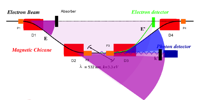
Figure 18: Illustration of suppression of synchrotron radiation background with fringe field modifying field plates P1-P4 attached to dipole magnets D1-D4. A combination of reduced magnetic field seen by the photon detector and absorbing material attenuates synchrotron radiation flux to negligible levels [12].

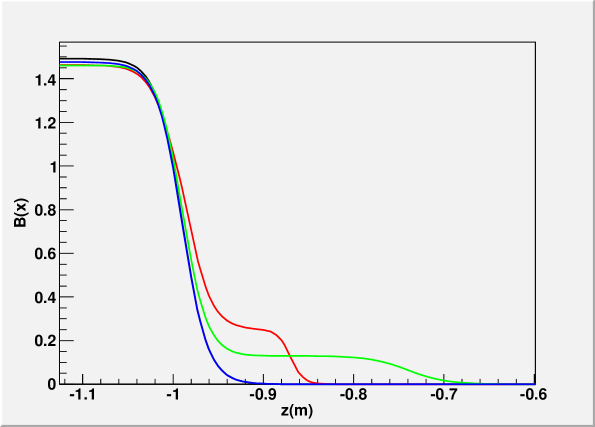
Figure 19: The effect on the fringe field of the dipole magnets due to the addition of the field plates. Shown are magnetic field strengths in T seen by the electron beam at 11 GeV for the basic dipole in blue, addition of short plates P1/P4 in red, and addition of long plate P3/P4 in green.

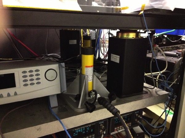
Figure 20: The optics table has been raised to the 12 GeV upgrade configuration. New vibration isolators with the correct height replace old leaky isolator legs.

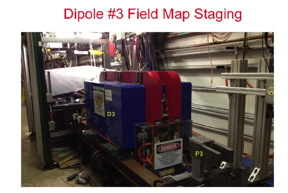
Figure 21: The 3rd dipole magnet in the Compton Polarimeter chicane being staged for field mapping. Shown in the foreground are the field plates P3 for synchrotron radiation suppression.

Engineering design of the 12 GeV upgrade has been completed. Fabrication of all components is complete and all parts are in house. The old beam line has been dismantled. As shown in Fig. 20, the optics table has been boxed up and raised to its 12GeV configuration with new isolator legs. The 2nd dipole magnet has been raised to its final location. The third dipole magnet has been rolled out of its place and is being staged for field measurements as shown in Fig. 21. Three sets of both integral and differential field measurements are planned. The basic dipole will be mapped first followed by the addition of P1 and P3 respectively. The integral field measurements are being carried out by Bagget et al. of the JLab magnetic measurement group using a stretched wire technique. Differential measurements with a hall probe 3D mapper will be carried out by Jones et al., University of Virginia, following the integral measurements.

The 12 GeV upgrade is on track to be completed in 2013. Commissioning with the upgraded CEBAF first beam delivery to Hall A are planned for early 2014.

2.2.5 Conclusion

As we wind down the 6 GeV operations of the Hall A Compton polarimeter and welcome the 12 GeV era, it is worthy of note that the green laser upgrades of the Compton polarimeter for 6 GeV operations have been immensely successful. The upgraded polarimeter was put into operation successfully for the recent PReX, DVCS, and g2p experiments. The green FP cavity far exceeds design goal by achieving upwards of 10 kW intra-cavity power. The green cavity along with the GSO photon calorimeter with integrating data acquisition system has provided the first set of high precision polarimetry results. Recent development in high speed counting data acquisition will further enhance the accuracy of the Compton polarimeter. Lackluster performance of the electron detector will get a boost with new collaborators from University of Manitoba and Mississippi. The 12 GeV upgrade project construction is proceeding well with initial operation expected in early 2014.

2.3 Polarized ³He Target

Polarized ³He Target: Status, Progress and Future Plan

contributed by J. P. Chen for the polarized ³He group.

The polarized ³He target ${}^{\cite[cite]{[\@@bibref{}{web}{}{}]}}$ was successfully used for fourteen 6 GeV experiments GDH ${}^{\cite[cite]{[\@@bibref{}{e94010}{}{}]}}$, GMn${}^{\cite[cite]{[\@@bibref{}{e95001}{}{}]}}$, A1n${}^{\cite[cite]{[\@@bibref{}{e99117}{}{}]}}$, g2n${}^{\cite[cite]{[\@@bibref{}{e97103}{}{}]}}$, Spin-duality${}^{\cite[cite]{[\@@bibref{}{e01012}{}{}]}}$, Small-Angle-GDH${}^{\cite[cite]{[\@@bibref{}{e97110}{}{}]}}$, GEn ${}^{\cite[cite]{[\@@bibref{}{e02013}{}{}]}}$, Transversity)${}^{\cite[cite]{[\@@bibref{}{transversity}{}{}]}}$, $A_{y}$-DIS${}^{\cite[cite]{[\@@bibref{}{AyDIS}{}{}]}}$, d2n${}^{\cite[cite]{[\@@bibref{}{d2n}{}{}]}}$, $A_{y}$-QE${}^{\cite[cite]{[\@@bibref{}{Ay}{}{}]}}$, $(e,e^{\prime}d)$${}^{\cite[cite]{[\@@bibref{}{target:e05102}{}{}]}}$ and $A_{y}$-$(e,e^{\prime}n)$${}^{\cite[cite]{[\@@bibref{}{e08005}{}{}]}}$.

The polarized ³He target initially used optically pumped Rubidium vapor to polarize ³He nuclei via spin exchange. Typical in-beam (10-15 $\mu$A) polarization steadily increased from $~{}30\%$ ${}^{\cite[cite]{[\@@bibref{}{slifer}{}{}]}}$ to over $40\%$ ${}^{\cite[cite]{[\@@bibref{}{target:Zheng}{}{}]}}$ when target cells were extensively tested and selected. A new hybrid technique for spin-exchange which uses a K-Rb mixture${}^{\cite[cite]{[\@@bibref{}{hybrid}{}{}]}}$ increased the in-beam polarization to over $50\%$ (close to $60\%$ without beam), due to the much higher K-³He spin exchange efficiency [18]. The new hybrid cells also achieved significantly shorter spin-up times ($<5$ hours compared to $<10$ hours for pure Rb cell) [19]. Further improvement in polarization was achieved recently for the transversity series of experiments by using the newly available high-power narrow-width diode lasers (Comet) instead of the broad-width diode lasers (Coherent) that have been used in the previous experiments. The target polarization improved significantly to $55\%$ with up to 15 $\mu$A beam and 20-minute spin-flip and over $60\%$ in the pumping chamber. Without beam the target polarization reached over $70\%$.

The earlier experiments used two sets of Helmholtz coils, which provided a holding field of 25-30 Gauss for any direction in the scattering (horizontal) plane. The transversity experiment also required vertical polarization. A third set of coils provide the field in this direction. These three sets of coils allow polarization in any direction in 3-d space. Target cells were up to 40-cm long with a density of about 10 amg (10 atm at $0^{\circ}$). Beam currents on target ranged from 10 to 15 $\mu$A to keep the beam depolarization effect small and the cell survival time reasonably long ($>3$ weeks). The luminosity reached was about $10^{36}$ nuclei/s/cm².

Fast target spin reversals are needed for the Transversity experiment (every 20 minutes). The fast spin reversal was achieved with Adiabatic Fast Passage (AFP) technique. The polarizing laser spin direction reversal was accomplished with rotating 1/4-wave plates. The polarization loss due to fast spin reversal is less than $10\%$ relative depending on the AFP loss and the spin up time. The improvement of spin up time with the hybrid cell has significantly reduced the polarization loss due to the fast spin reversal. With the BigBite magnet nearby (1.5 m) and a large shielding plate, the field gradients are at the level of 20-30 mg/cm, which is about a factor of 2 larger than that without the BigBite magnet. These field gradients lead to about $0.5-0.7\%$ AFP loss. Correction coils could reduce the field gradients. However, it was found that when the field gradients reduced to less than $10-15$ mg/cm, masing effects${}^{\cite[cite]{[\@@bibref{}{romalis}{}{}]}}$ started, which caused a significant drop in the target polarization (from $70\%$ to $<60\%$). We decided to leave the field gradients high by tuning off the correction coils to avoid the masing effect.

Two kinds of polarimetry, NMR and EPR (Electron-Paramagnetic-Resonance), were used to measure the polarization of the target. While the EPR measurement provides absolute polarimetry, the NMR measurement on ³He is only a relative measurement and needs to be calibrated, often with NMR on water. Water NMR provides an absolute calibration since the proton polarization at room temperature is known. The water signal is very small and it is often a challenge to control systematic uncertainties below a few percent level. The uncertainty achieved with Rb only cell (before GEn) was $3\%$ for both EPR and NMR with water, while for hybrid cell (GEn and transversity series) was $5\%$ relative. The main reasons for the larger uncertainty with the hybrid cell were due to 1) the higher operating temperature ($230^{\circ}$C) while the existing measurements of the EPR calibration constant ($\kappa_{0}$) were only performed at below $200^{\circ}$C; 2) the large uncertainty in the diffusion due to the longer transfer tube. With the exception of the GEn experiment, all experiments have both EPR and NMR with water calibration and the two methods agree well within errors. The GEn experiment used a magnet box instead of the standard Helmholtz coils to provide the main holding field. Online polarimetry during GEn was accomplished using the NMR technique of adiabatic fast passage, as had been done previously. The calibration of the NMR, however, was done solely using EPR. This was because the study of NMR signals from water were unsuccessful, due largely to hysteresis effects associated with the iron-core magnet. The lack of a water calibration, however, did not contribute significantly to the final errors of the experiment.

The latest analyses of the polarimetries (Fig. 22) were done by Yi Zhang${}^{\cite[cite]{[\@@bibref{}{YiZ}{}{}]}}$ (with cross check by Jin Huang and help from Yi Qiang) for the transversity experiment, by Yawei Zhang for $A_{y}$ and by Matthew Posik for the $d_{2}^{n}$ experiment. The polarization results were cross-checked with a measurement of the e-³He elastic asymmetry, showing an agreement at a level of about $5\%$.

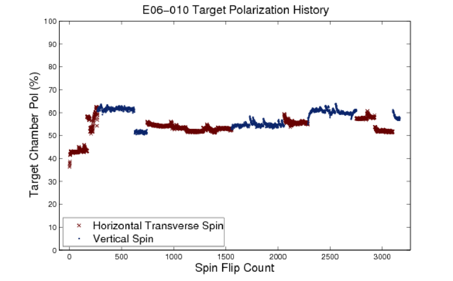
Figure 22: The polarized ³He target performance with $10-15\mu$A and spin-flip during the transversity experiment.

After the last set of polarized ³He target experiments in the 6 GeV era (the transversity series), the target was moved back to the target lab in the EEL building and was set up to continue tests and R$\&$D. EPR measurements with D1 line was tested and performed successfully for the first time. Fast spin reversal with field rotation was tested and it was proved in principle that spin reversal speed could be increased significantly by using field rotation. Several tests were performed aiming to help polarimetry analysis. Careful study was done to understand the diffusion effect (the polarization changes from the pumping chamber to the target chamber due to temperature gradients), which was one of the dominate uncertainties in the polarimetry. Systematic studies were also performed to study the temperature dependence of polarization decay (life) time and spin up time. Masing effects were also studied. These studies provide some basic information for our understanding and control of systematic uncertainties.

Further R&D efforts were focussed on meeting the need the requirements for the planned 12 GeV experiments. Seven polarized ³He experiments are approved with high scientific rating (three A and four A-). Two experiments using the SoLID spectrometer${}^{\cite[cite]{[\@@bibref{}{SoLID}{}{}]}}$ will be a few years away and only require the already achieved performance. The following discussion describes the requirements of remaining five experiments. The first group of experiments (A1n-A${}^{\cite[cite]{[\@@bibref{}{A1nA}{}{}]}}$, d2n-C${}^{\cite[cite]{[\@@bibref{}{d2nC}{}{}]}}$, SIDIS-SBB${}^{\cite[cite]{[\@@bibref{}{SIDIS-SBB}{}{}]}}$) ask for improvements of about a factor of 3-4 in figure of merit over the best achieved performance and the second group (A1n-C${}^{\cite[cite]{[\@@bibref{}{A1nC}{}{}]}}$ and GEN-II${}^{\cite[cite]{[\@@bibref{}{GENII}{}{}]}}$) demand improvement of about a factor of 6-8 in figure of merit. With the limited resources (engineering/design manpower and funding) available to meet the challenge of the 12 GeV experiments, a plan has been developed to have a two-stage approach for the target upgrade. In the first stage, we aim to have a 40-cm 10 amg target capable of handling 30 $\mu$A of beam current with an in-beam target polarization of $60\%$. Polarization measurements aim to reach a precision of $3\%$. This target will meet at least the acceptable requirements of the first group. To reach this goal, we plan to make full use of the existing polarized ³He setup from the last set of 6 GeV running and make the necessary modifications as outlined in the following steps:

• Using cells with convection flow

• Using a single pumping chamber with 3.5-inches diameter sphere

• Shielding the pumping chamber from radiation damage

• Using pulsed NMR, calibrated with EPR and water NMR

• Measure EPR calibration constant $\kappa_{0}$ to higher temperature range covering the hybrid cell operation temperature (user responsibility)

• Metal end-windows desirable (optional for $30\mu$A, must for higher current, another user R&D project).

The first running of a polarized 3He experiment is expected to be in 2016. Our goal is to have the first-stage (moderately-upgraded) target system ready by early 2016. The goal can be reached with a moderate cost and a moderate engineering/designing/supporting manpower.

The second stage is to meet the needs of A1n-C and GENII-A experiments. It will be a 60-cm 10 amg target capable of handling 60 $\mu$A beam with a polarization reaching $65\%$. It requires at least to double the pumping volume by using a double-pumping-chamber design. Metal end-window or metal cell will be needed. To increase the target cell length from 40 cm to 60 cm, the holding field coils need to be re-arranged. The small set of coils needs be replaced by the large set of coils (used for vertical pumping during transversity).

The polarized ³He program at JLab has been very successful in the 6 GeV era, mainly due to a collaborative effort among the users and JLab. R&D efforts at the user polarized ³He laboratories have contributed critically to the continuous improvements over the years. This successful model is continuing into the 12-GeV program. R&D by the user groups have already made significant progress. The UVa (Gordon Cates) group has developed and tested the convection cell concept and demonstrated that it works [28]. They also developed a pulsed NMR system and tested it at UVa. R&D on metal end-window is also underway by the UVa group. One important item for polarized ³He is the narrow width laser. Comet laser production has been discontinued. Investigation is on-going to find a suitable replacement. William and Mary (Todd Averett) group has performed first tests of a new laser from a new vendor QPC.

R&D activities at the JLab target lab has been on-going for the upgrade. A graduate student (Jie Liu) and a postdoc (Zhiwen Zhao), both from Xiaochao Zheng’s group at UVa, have been actively working in the target lab. In addition to the tests necessary to understand systematics for target polarization measurements, a pulsed NMR system was developed at the JLab target lab. It has been tested to work well (Fig. 23). Systematic study to understand the pulsed NMR system is underway. A new laser from QPC is undergoing tests. One convection cell with single 3.5 inch diameter pumping chamber has been manufactured. After initial tests at UVa, it is now being set up for full tests at JLab (Fig. 24).

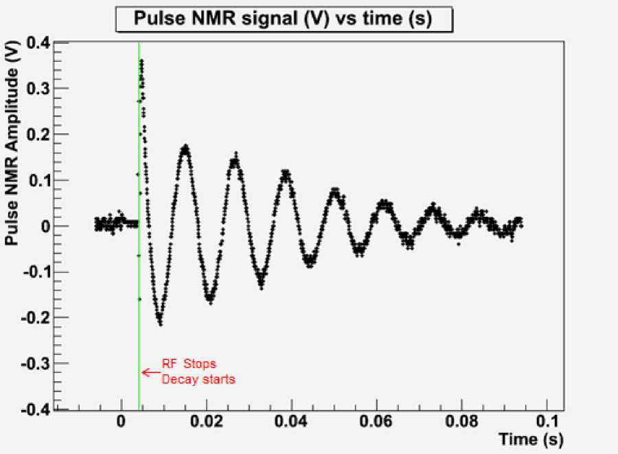
Figure 23: Pulsed NMR signal from JLab target lab test.

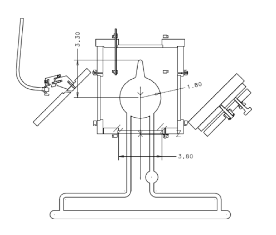
Figure 24: Convection cell test setup at JLab target lab.

2.4 Data Analysis

Data Analysis

contributed by J.-O. Hansen.

2.4.1 Podd (ROOT/C++ Analyzer) Status

For several years now, the main Hall A data analysis package, “Podd” [1], has been in a stable production state. All experiments that ran during 2011/2012 have used Podd for analysis. Over the past year, updates to Podd have consisted mostly of small bug fixes and usability improvements. However, there have been a few noteworthy upgrades and changes:

• Helicity decoder classes for the Qweak helicity scheme were contributed by Julie Roche.

• Additional VME front-end module decoders were included by Larry Selvy.

• A system for automatic run-time string replacement in the various text input files was implemented, encapsulated in the THaTextvars class.

• Previously existing string size limits in the EPICS classes have been completely lifted.

• Support current ROOT and Linux versions: ROOT versions up to 5.34 and gcc compilers up to version 4.7 (as used in Fedora 17, for example) have been tested.

• Experimental support for Mac OS X has been added.

• Version management of the code has been moved from the obsolete CVS system to git.

The THaTextvars system mentioned above allows users to write generic text input files (database, cut and output definitions) that are independent of actual spectrometer and module names used in the replay setup. These files may now contain macro names that are replaced at run time with values set in the replay script. Moreover, replacement macros may contain entire lists of module names, not just single ones. As a result, it is no longer necessary to create multiple text files, or duplicate sections within a text file, if these parts only differ by module name, which is frequently the case. This system is optional and fully backwards compatible with existing input files.

Additionally, a much-improved version of the HRS VDC analysis code was developed for the APEX test run in 2010. This code finally addresses the issue of ambiguities due to multiple hits in the VDCs, which occur at high singles rates, largely due to accidental coincidences during the relatively wide (ca. 400 ns) drift time window. The new algorithm is able to suppress background from accidental coincidences by at least a factor of 5 by exploiting the timing information from the group of wires in a hit cluster. A non-linear, 3-parameter fit to the drift times is performed to extract the approximate time offset of the cluster hit with respect to the main spectrometer trigger. This new VDC class is not yet part of the official Podd release, but is available in the git repository. It will be included in a future releases, once the code has been cleaned up and documented.

The current version of Podd is 1.5.24. Downloads and documentation is available, as usual, from the main Hall A web page.

2.4.2 External Software Review

In June 2012, an external review of the status of the laboratory’s online analysis software and computing facilities was held at Jefferson Lab. The review focused on the suitability of the different halls’ software and analysis plans for the 12 GeV era. With respect to Hall A, the committee found us generally well prepared, and considered our plans sound. Naturally, there were several recommendations, which are summarized here:

1. In general, all halls were encouraged to continue and improve good software development practices, such as automatic code builds, use of standard code evaluation tools, and development of standard software validation procedures.

2. The main suggestions for our Hall A analysis package Podd were

   • Try to implement automatic event-level parallelization in keeping with the prevalent industry trend toward increasingly large-scale multi-core processing.

   • Collaborate with Hall C to develop a common core analysis package.

3. Finally, it was recommended to carry out a more detailed evaluation of performance and limitations of the track reconstruction algorithm for SuperBigBite.

Many of the suggestions under item 1 are already being employed in Hall A, although we can do better in some areas, such as developing a more comprehensive test suite. The recommendation under item 2 are well taken and have actually been on our “like to do” list for years, along with other items, such as overall performance improvement and more modularity. They will be addressed with the upcoming release of Podd 2.0, described below. Item 3 is project-specific.

2.4.3 Collaboration with Hall C

Already early in 2012, Hall C decided to rewrite their analysis software for 12 GeV experiments in an objected-oriented way, using C++ and ROOT, and to base this project on our Podd package. This decision gained further momentum by the outcome of the software review, discussed above. For several months now, we have been consulting with Hall C in implementing the code necessary to support their hall’s equipment within the framework of the Podd analyzer. This collaboration has proven fruitful, as expected. Several limitations of the current Podd design were exposed, and Hall C is similarly discovering inefficiencies in their existing analysis methods and algorithms. Effectively, the porting of the Hall C analyzer to the Podd framework has sparked a thorough code review and general rethinking of analysis methods for both halls. The end result will clearly be improved software quality.

There is now a task list of architectural improvements to Podd that will permit the use of a core library with hall-specific libraries as add-ons. Development of a number of smaller new features is in progress, which will be included in Release 1.6 of Podd, expected in early 2013.

2.4.4 12 GeV Software

In preparation for 12 GeV data taking, we plan to develop a major new version of Podd, Release 2.0, for the second half of 2013. This is intended to be the core software to be used for the first 12 GeV experiments in Halls A and C. Podd 2.0 will probably include most and hopefully all of the following:

• Automatic event-level parallelization of the core analyzer.

• Significantly improved speed of writing ROOT output files.

• Decoders for the pipelined JLab 12 GeV electronics.

• SQL database backend.

• VDC multicluster analysis, mentioned in section 2.4.1 above.

At this time, it appears as if most of the 12 GeV experiments planned for Hall A anticipate to use Podd as the basis of their offline analysis. (The one notable exception is the Møller parity-violation experiment.) Consequently, the considerable effort we will spend over the next year or two on updating our analysis software will be a sound investment in the future.

2.4.5 Computing Infrastructure

Many improvements to the lab’s and the hall’s computing infrastructure occurred in 2012. A few highlights, which may be of particular benefit to Hall A users, follow:

• A new /volatile disk area was commissioned by the Computer Center. This is a very large and very fast storage area with an automatic cleanup policy [2]. Its behavior is a mix of that of the old /scratch area, with no storage guarantees, and that of /work, with a guaranteed safe space. Like /work, /volatile is not backed up. This new space is ideal for large output files that need to survive for a few weeks to a few months. It is readable and writable from the compute farm.

  Currently, 170 TB of space are available for all halls together (some dedicated to certain projects who paid for the disk hardware). Hall A currently has a reservation of 10 TB (guaranteed space) and a 30 TB quota. The quota is soft, i.e. can be briefly exceeded if unused space is available. More space will be requested once our demand rises.

• Several old machines in the Hall A counting house were (or will soon be) replaced in favor of modern hardware. The function of the two DAQ machines, adaql1 and adaql2, is being migrated to adaq1 and adaq2, each with over 3 TB of very fast raw data staging disks and 6-core processors. The local file server, adaql10, has been replaced with a newer machine, chafs, that currently offers 20 TB of work space for online analysis. Any new server functions should be put onto this machine.

• Hall A now has a dedicated MySQL database server, halladb.jlab.org, which is accessible from anywhere within the lab. (We may also request offsite access, if needed.) This server currently contains a copy of the online databases that used to stored on the now-decommissioned counting house computer adaql10. A new backup server has been set up in the counting house as well; it will be synchronized with the central server.

Due to increased cyber security demands, the counting house computers as well as the hall networks will stop being accessible with direct ssh from the general computing networks (i.e., user desktops, CEBAF Center, etc.) by late December 2012. Access from these “remote” networks will require a two-factor authentication token and login via a gateway, as is already the case for the accelerator networks. This change only affects remote access; users at terminals in the counting house or in the hall will see no changes.

2.5 HRS Detectors

Detector package of the High Resolution Spectrometers

contributed by B. Wojtsekhowski, Hall A, Jefferson Lab.

Introduction

The detector package of the High Resolution Spectrometers is described in the Hall A instrumentation paper [1]. Here we have listed upgrades which are underway in 2012-2013. After 15 years of operation, some of the detectors are losing performance due to aging. Some improvements in the detectors have become possible due to progress in electronics. A few years ago we constructed and implemented the S2m scintillator hodoscopes in each HRS, which have superior time resolution enabling reliable PID in several experiments from 2004 to 2010. A program of HRS detector “hardening” was approved in 2010. It includes an upgrade of the VDC front-end electronics, replacement of the aged S1 hodoscope, and refurnishing of the A1 aerogel counter (n=1.015). The initial Hall A FY12 plan anticipated significant advances in the hardening program. However, the final plan, due to a funding redistribution in FY12, provided only minimum resources for the HRS hardening.

In 2013 the VDC electronics upgrade will be implemented by re-using the A/D cards donated by W&M after completion of the Qweak experiment. Two new S1 hodoscopes are 40-90% completed, but during 2013 they will be on hold due to a lack of funding for manpower and PMT procurement. The A1 refurnishing has been postponed indefinitely because none of the currently approved experiments plans to use HRS(s) for hadron detection.

2.5.1 VDC electronics

The previously used front-end VDC electronics is a LeCroy 2735DC card based on a 20-year-old design. Due to the open design of the VDC frames (all of the them are non-conductive), the output signals of the A/D cards induce large feedback and often cause so-called oscillation. A high threshold level in the A/D cards required for suppression of such oscillation leads to a high value of HV on the chamber. For the Ar-Ethane(62/38) gas mixture, the operational HV is of 4000 V. The threshold level defines the required gas multiplication factor and average anode current at the given rate of the tracks. At the current level of 100 $\mu$A the VDC operation become unstable. For the GEn (E02-013) experiment, the A/D cards based on the MAD chip were constructed for use in the BigBite spectrometer wire chambers [2]. Two key advantages of those cards are a low amplitude of the output signal (LVDS) and reduced noise of the front elements. The resulting reduction of the threshold is about 5 for the input charge.

In addition to the upgrade of the VDC front-end cards, we are going to implement the sparsification window by using 1877S FastBus TDCs (procured by Carnegie-Mellon University from CLEO for a symbolic $50 per module). These modules were tested in 2012 and have already been installed in the HRS DAQ crates. The sparsification window of 400 ns will allow significant reduction of the event size at a large rate of the particles and lower dead time of DAQ.

2.5.2 Front FPP chambers

The HRS Focal Plane Polarimeter, FPP is installed in the HRS-left spectrometer. The FPP includes four large drift chambers of straw tube design. Two chambers constitute the front group and two others the rear group. The adjustable thickness carbon analyzer is installed between the groups. Many highly rated experiments have been performed using the HRS FPP system. Sometimes operation of FPP was difficult, mainly due to gas leakage from the chambers, which was very high. Even with a huge gas flow of 50 l/h, the chambers were unstable due to frequent HV trips.

Analysis of the problem performed in 2010 showed that the main leak is due to misalignment in the attachment of the gas lines into the rubber plug of the straw tubes. The proper modification was developed and all parts have been procured. Additional improvements have been made in the HV distribution panel (a single board) and the gas distribution configuration (a parallel input and an open output). In 2013 these upgrades of the front FPP chambers will be implemented. The first use of the upgraded chambers will be in the GMp experiment (E12-07-108) [3].

2.5.3 Shower Calorimeter Trigger

The HRS-right shower calorimeter was constructed together with the custom summing electronics for trigger purposes by the University of Maryland. However, those sums were never used in the experiments, and the electronics were later removed. In 2011 we restored the summing electronics and have a plan to use both the pre-shower and the total energy signals in the trigger. These signals allow us an additional measurement of the trigger efficiency and efficient pion rejection on the trigger level. Similar electronics will be assembled on the HRS-left.

2.5.4 Status of the S1/S2 hodoscopes

The HRS original trigger counters were made of thin plastic scintillator (5 mm BC408) to allow detection of low energy hadrons. Each S1 and S2 hodoscope has six counters with about a 5 mm overlap between them. A large aspect ratio (of 60:1) of the scintillator cross section requires a long twisted light guide resulting in reduced light collection efficiency. In their virgin state, these counters had in the cosmic ray signal about 120 photo-electrons per PMT, and the time resolution per counter was about 0.30 ns ($\sigma$), which currently degrades to about 0.6-0.7 ns.

The S2 hodoscope, which in fact doesn’t need to be thin, was replaced in 2003 by a 16-paddle hodoscope, S2m(odified) made of 50 mm fast plastic scintillator EJ-230 [5] (see for details [4]) with a time resolution of 0.10 ns ($\sigma$) [6]. Last year we finished construction of a new 16-paddle hodoscope, S1m(odified) made of 10 mm plastic scintillator (EJ-200) and XP2262B. The optimized shape of the light guide and doubled thickness resulted in a time resolution of 0.20 ns. The mounting frame for this hodoscope has also been designed and constructed. For the second, S1f(ast) hodoscope, we selected a fast scintillator (EJ-230), a novel design of the light guide, and the high performance PMT R9779 [7]. This allowed us to get about 300 photo-electrons per PMT and reach a time resolution of 0.08 ns with only a 5 mm thickness of the scintillator. The components of these counters have been produced. However, completion of the S1f hodoscope requires procurement of the 32 PMTs and manpower for assembling the counters and mounting frame which will not be available in 2013.

2.5.5 Status of the Gas Cherenkov counters

The performance of the HRS Gas Cherenkov counters, GC, has degraded by a factor of 2 since commissioning. During the last 6-GeV experiment, the average number of photo-electrons was only about 5. The plan of GC refurnishing includes re-coating of the mirrors and implementation of the 5” Hamamatsu PMTs. The latter is not possible in 2013, and we will select the best available 5” PMTs from those used in the two existing aerogel counters.

2.5.6 Active sieve slit counter

A long-standing problem of the high energy magnetic spectrometers is the sieve slit calibration for the positively charged particle configuration. For the negatively charged particle configuration, the sufficiently thick sieve slit allows selection of the holes when the electron tracks are identified in the focal plane. In contrast, for the positively charged particle configuration, the flux of positrons is too small to compete with the secondary positrons produced in the sieve slit body.

We have developed an active sieve slit device based on a scintillator fiber hodoscope. It includes 32 fibers in the X-direction and 32 fibers in the Y-direction, all connected to the 64-channel maPMT. The detector is placed in a vacuum between the target and the first magnet of the spectrometer. The position of the detector is remotely controlled. The first use of this device will be in the APEX experiment (E12-10-009) for calibration of the positron arm magnetic optics.

2.6 Super Bigbite

The SBS Program in Hall A

contributed by John J. LeRose.

2.6.1 Introduction

The Super BigBite Spectrometer (SBS) while in principle consisting of a very simple, single dipole based magnetic spectrometer is actually a collection of many devices that will be used in conjunction with SBS to achieve the desired Physics goals. What follows describes the plans, as presented to and approved by DOE, to construct the basic spectrometer and a limited set of detectors needed to get started on the envisioned research plan.

2.6.2 Program Description

Using the Super Bigbite Spectrometer Program Management Plan Jefferson Lab and its collaborative partners will produce key components of the research equipment required to conduct a series of elastic nucleon electromagnetic form factor measurements.

Each of the measurements will use the electron beam from the upgraded 12 GeV  CEBAF accelerator. The three experiments include:

• A measurement of to $Q^{2}=10~{}\mathrm{GeV}^{2}$ using the double polarization beam-target technique (E12-09-016)

• A measurement of to $Q^{2}=12~{}\mathrm{GeV}^{2}$ using the double polarization beam-recoil-polarimeter technique (E12-07-109)

• A measurement of to $Q^{2}=13.5~{}\mathrm{GeV}^{2}$ by determining the cross-section ratio for the two reactions $d(e,e^{\prime}n)$ and $d(e,e^{\prime}p)$ (E12-07-109).

These experiments along with precise data from the experiment (E12-07-108) will determine all four elastic electromagnetic nucleon form factors, as well as making possible a flavor separation. Because all the elastic form factors drop off so quickly at high values of $Q^{2}$, the three experiments all depend critically on both high luminosity as well as relatively large acceptance.

The three measurements each require a somewhat different experimental set-up. They are designed so that they can be accomplished using largely common components that can be rearranged into the required configurations. Collectively, this set of components is called the “Super Bigbite Spectrometer”. The research program will also take advantage of the equipment associated with the existing BigBite spectrometer that resides in Jefferson Lab’s experimental Hall A, and some hardware under construction for other approved experiments.

The SBS focuses on large-acceptance detection, makes use of an existing magnet, and will utilize a detector package with Gas Electron Multiplier (GEM) tracking detectors. GEM technology has advanced significantly in recent years. A collaboration with INFN-Rome has already begun development of the front-end GEM’s and data-acquisition electronics such that the final design is essentially in-hand.

2.6.3 Program Approach

The SBS Program will consist of three separate, but interrelated Projects.

The first Project, SBS Basic, involves the acquisition of an existing magnet (48D48 magnet from Brookhaven National Lab) and the associated work of preparing it for use during the SBS research program. The effort includes modifications to the magnet, including machining a slot in the yoke for beam passage, field clamps, and a solenoid to reduce the transverse magnetic field on the beam line, the design and development of the infrastructure needed to run the magnet, and the construction of the platform on which it will stand.

The second Project, Neutron Form Factor, involves the construction of twenty-nine GEM detector modules with associated front-end and DAQ modules to meet the requirements of the approved neutron form factor measurements.

The third and final Project, Proton Form Factor, involves the construction of thirty-five GEM detector modules with associated front-end and DAQ modules, a sophisticated trigger system, and the addition of pole shims for increased magnetic field integral to meet the requirements of the approved proton form factor measurements.

The three Projects that comprise the SBS Program include construction and commissioning of the individual hardware systems. Installation in the Hall, as with essentially all other experiments, will follow the as yet undetermined beam schedule and will use Hall A Operations funding.

2.6.3.1 The SBS Basic Project

The SBS spectrometer itself is a large dipole made from a modified 48D48 magnet that will be obtained from Brookhaven National Laboratory for the cost of disassembling and moving it. The modifications included in this project are:

• Machining a slot in the return yoke to allow passage of the beam at small scattering angles

• New coils to accommodate the new geometry

• Field clamp to reduce the field at the target

• Providing a small solenoid to minimize the magnetic field in the beam slot around the field clamp

The magnet will require support structures to hold it and the detectors. The support structure will be versatile enough to accommodate the various angles anticipated by the future experimental program. The magnet will also require a power supply with all necessary infrastructures to power the magnet (water, AC power, busses, safety interlocks).

For this project, spread over fiscal years 2013-2015, $1,693k, including 28% contingency, has been budgeted from JLab Physics Division capital funds.

At this time (12/3/2012) design work has begun on the magnet modifications (including yoke modifications and new coils), and the support structure to hold the magnet. It is expected that the steel and coil modification drawings will be completed by February 1, 2013. This will allow us, by the present schedule, two months to negotiate a contract with a vendor to make the needed modifications to the steel and have the steel shipped directly to the vendor from Brookhaven.

2.6.3.2 The Neutron Form Factor Project

In this project the following will be constructed:

• Gas Electron Multiplier (GEM) tracking detectors (UVa), 29 modules

• Front-end and data-acquisition electronics (UVa) to accompany these modules

• Electronics Hut, Detector Frames, and Materials needed to construct the Lead Tube Shielding, and the Lead Tube Platform for the beamline (JLab)

At the present time (12/3/2012), although not formally a part of the Neutron Form Factor Project, an intensive effort is underway at UVa, under the guidance of Nilanga Liyanage, to develop the techniques and technology needed to successfully manufacture these detectors. It is expected that those techniques and technologies will be finalized by April 2013 at which time ordering of the needed parts for production will begin.

For this project, spread over fiscal years 2013-2015, $1,572k, including 30% contingency, has been budgeted from JLab Physics Division capital funds.

2.6.3.3 The Proton Form Factor Project

In this project the following will be constructed:

• Gas Electron Multiplier (GEM) tracking detectors (UVa) (35 modules)

• Front-end and Data Acquisition Electronics to accompany these GEM modules (UVa)

• A Trigger (RU)

• Pole shims (JLab)

• Exit field clamp (JLab)

For this project, spread over fiscal years 2014-2017, $1,582k, including 27% contingency, has been budgeted from JLab Physics Division capital funds.

2.6.4 The Future

At the end of these three projects Hall A will have a unique and versatile, large acceptance ($\Delta\Omega\approx 70~{}\mathrm{mstr}$ at $15^{\circ}$, $-12.5\% < \delta < 12.5\%$), high luminosity (up to $10^{39}~{}\mathrm{s}^{-1}\mathrm{cm}^{-2}$) capability suitable for many future experiments.

2.7 Electromagnetic Calorimeter

Electromagnetic Calorimeter

contributed by C.F. Perdrisat, C. Ayerbe Gayoso, College of William and Mary,

M.K. Jones, Jefferson Lab,

V. Punjabi, NSU, E. Brash, CNU.

2.7.1 Detector

An electromagnetic calorimeter, EMC, is required for the GEp(V) experiment, a measurement of the $G_{Ep}/G_{Mp}$ form factor ratio up to Q²=15 GeV² (original proposal, 2007) by the recoil polarization method $\vec{e}p\rightarrow e^{\prime}\vec{p}$. The subsequent rating of the proposal resulted in a decrease of the maximum Q² to 12 GeV². In GEp(V) both electron and proton need to be detected, and a trigger defined with high threshold on the electron (and proton) energy. Needing a threshold of 80-90% of the electron energy to reduce the DAQ rate presents a challenge as illustrated in Fig. 25: the electron energy range for Q²=12 GeV² is 3.5 to 6 GeV; the gain of the PMTs will have to be adjusted according to the distribution of energy over the front face of the calorimeter, and according to the radiation dose received by the individual bars, which is not uniform. To reduce the low-energy background on the EMC, a 20-cm aluminum block is placed in front of the lead glass. This has the unfortunate side effect of degrading the energy resolution of the calorimeter, since the shower start in the aluminum block. This leads to energy resolution which is only 1.5$\sigma$ of the desired electron energy threshold and loss of about 14% of the triggers.

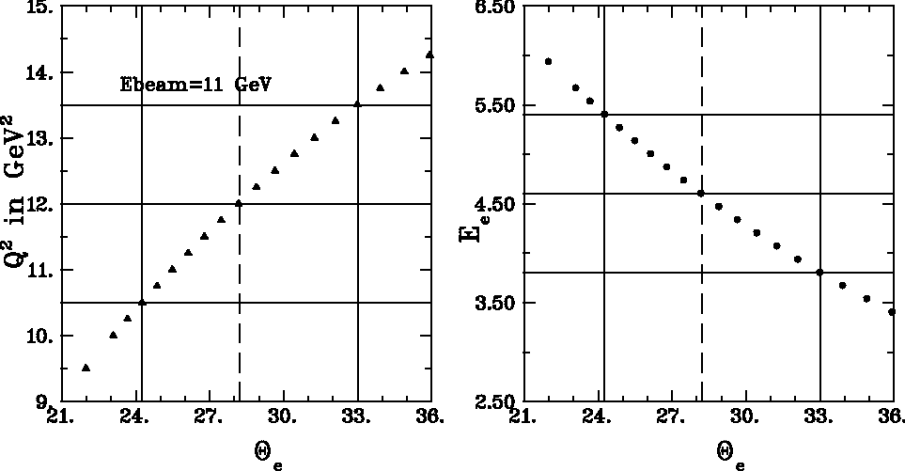
Figure 25: Left figure: Plot of Q² versus the scattered electron’s angle, $\theta_{e}$. Right figure: The scattered electron’s energy,E_e, versus angle. In both plots, the vertical dashed line highlights the value of $\theta_{e}$ at Q² = 12 GeV².

Off-line analysis will require accurate determination of the angle of the electron, to sharpen background rejection using the two-body angle correlation in elastic ep. The BigCal spatial resolution has been typically 0.5 cm (1$\sigma$). A new calorimeter will be equipped with a coordinate detector, originally designed as two plane of GEMs, with readout of the vertical coordinate only; the resolution in the vertex position defined by the proton arm (and the 40 cm long target) is not sufficient to justify reading the horizontal coordinate.

The beam intensity and energy, target length and detector angles required for Q²=12 GeV² are such that the rate of gain loss for the lead glass of GEp(III) calorimeter will be 1̃3 times larger than in GEp(III). This has lead to the estimate that recovery of the leadglass transparency after 7 hours of beam requires one hour a UV irradiation curing. After the curing, a check of the PM gain is required; together, irradiation and PM re-tuning represents a minimum of 2 hour loss of data taking every 8 hours, or 25%.

In view of this significant loss of beam time or efficiency, we have been considering other options for a new electron calorimeter. Of particular interest is the sampling calorimeter design, in which the electron shower is sampled in a stack of scintillator and lead (or iron) plates, with the light collected in WLS plastic fibers running through the whole length off the stack; often called shashlik. Many such calorimeters exist, but we have concentrated our attention to the HERA-B setup, which contains a very large stack of shashlik elements that are not currently being used. This calorimeter was built at ITEP in Moscow. It consists of modules 11.2x11.2 cm² in cross section, and a thickness of 20 radiation lengths (X_o). A very good design for the new calorimeter would consist of either 300 or 432 such modules; the calorimeter, NewCal, would be located at an appropriate distance from the target to insure that all electrons elastically scattered with a proton accepted in the SBS proton arm, are contained in the e-calorimeter. To insure that the analog signals from all elements containing a shower are summed independently of where the electron hits, systematic overlap between neighbor modules, both horizontally and vertically, is required. Various schemes to achieve this requirement have been studied.

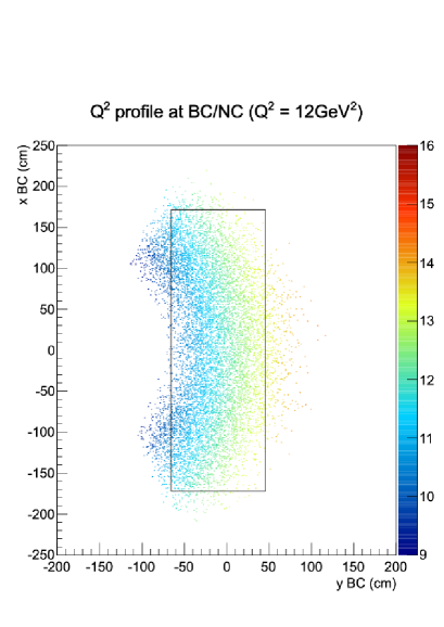
Figure 26: Q² profile at the NewCal for Q² = 12 GeV².

Figure 27: The unweighted (blue) and cross-section weighted (red) yields for Q² = 12 GeV²

2.8 Hadron Calorimeter

Hadron Calorimeter, HCAL-J

contributed by G. B. Franklin and V. Mamyan, Carnegie-Mellon University,

for the CMU, Catania, JINR, JLab collaboration.

The DOE review report of October, 2011, stated that, ”while not formally part of the SBS program, the HCAL calorimeter and its good performance are essential for the envisioned suite of experiments.” They found the design concept, based on the existing COMPASS HCAL1 detector appropriate and noted that ”the HCAL design appears to have adequate segmentation to provide sufficient angular constraints for the neutron program.” The report recommended the development of relevant HCAL specifications and quality control procedures. In response, specifications for the HCAL-J detector have been developed and numerous performance tests of prototype modules and materials have been performed as the first steps of developing realistic quality control specifications.

2.8.1 Detector Specifications

The design specifications of HCAL-J are determined by the requirements of the GEp, GMn, and GEn experiments. They are summarized as follows:

Size: The detector should have an active area of 160 cm x 330 cm to match the acceptance of the SBS. If allowed by budget considerations, a detector larger than this minimum size will be constructed to maintain resolution near the acceptance boundaries and to provide the improved performance associated with a larger time-of-flight distance.

Energy Resolution: The module design will be optimized to allow the use of a high threshold trigger to reject background events while maintaining high trigger efficiency for the real events. The goal will be to achieve efficiency greater than 95% with a trigger threshold set at 25% of the average signal.

Time Resolution: Simulations show timing requirements, combined with an RMS time resolution of 1.0 ns from the HCAL detector, would result in a trigger efficiency of 80% for the GEn experiment. This is acceptable as the minimum performance criteria, but the HCAL-J module geometry, scintillator materials, and waveshifters will be optimized to obtain a time resolution better than 1.0 ns RMS with an overall goal of achieving a time resolution closer to 0.5 ns RMS.

Angular Resolution: The detector will be designed to provide a spatial resolution of 8 cm RMS and thus the desired angular resolution of 5 mrad can be achieved by placing the detector 17 m from the target.

Gain monitoring: The detector will have an LED or laser-based pulser system that will allow in-situ monitoring of the PMT gains and facilitate data-acquisition testing.

2.8.2 Module Design

The HCAL-J detector design will be based on a modular construction similar to the existing HCAL1 detector used in the COMPASS experiment. Each module will consist of alternating layers of iron and scintillator. In use, the hadronic showers are formed in the iron and the scintillators sample the energy of the showers. The resulting scintillation light is director to PMTs using wavelength-shifter/light guides that run the length of each module.

Each module will have a 15 cm$\times$15 cm front face and will be approximately 1 meter in length. With this design, the 160 cm x 330 cm active area design criteria can be achieved by stacking 288 modules into an array 12 wide by 24 high. The individual modules will be constructed to allow this stacking by using the iron plates to transfer the load of the upper modules through the lower modules.

In order to make calorimeter suitable for the JLab energy range, 2-10 GeV, the thickness of scintillator plates will be increased from 0.5 cm to 1.0 cm while keeping the total length and number of plates the same. This increases the light yield but reduces the thickness of iron plates (from 2.0 cm to 1.5 cm) and therefore hadron detection efficiency. The energy resolution of a device with this design was simulated realistically by taking account light propagation in the wavelength shifter (WLS) and the PMT efficiency. For a hadron momentum of 2.7 GeV/c, energy resolution was found to be 42.3% and it gradually improves with increasing hadron momentum. The Geant4 simulation shows that 1.5 cm thick iron plates are thick enough to provide more than 95% hadron detection efficiency in the 2-10 GeV energy range when the hadron calorimeter threshold is 1/4 of the average deposited energy.

The position of the incident hadron is determined using an energy-weighted sum of the positions of the modules containing the corresponding hadronic shower. The resulting position resolution predicted from simulation is 5.5 - 3.0 cm for hadrons in the momentum range 2-10 GeV/c. The angular resolution of 5 mrad $\sigma$ can be achieved by placing the calorimeter about 12 m from the target. The predicted coordinate resolution at 40 GeV hadron momentum agrees with the resolution achieved by the COMPASS experiment (1.5 cm RMS).

2.8.3 Time Resolution Optimization

Time resolution is critical for rejecting background during form factor experiments. The goal resolution is 0.5 ns sigma and is most important for background separation at higher hadron momentum due to short time of flight.

To achieve the required time resolution, we will deviate from the COMPASS design in the choice of scintillator and wavelength shifter (WLS) materials. The choice of plastic scintillators is constrained by several factors, most important of which is the need to match emission spectrum of the scintillator with the absorption spectrum of the fast wavelength shifter . Fast wavelength shifters ( for example EJ-299-27 and BC-484 ) tend to have absorption spectra near the end of the UV and start of the violet range (350-400 nm). Since wavelength shifters are sensitive to light in the 350-400 nm range absorption, absorption of light in scintillator becomes problematic due to increased light absorption by the base material (PVT) of scintillators. Another problem is absorption and re-emission of light by scintillator fluor (PPO). The variation in the efficiency of the re-absorption and re-emission process as a function of spatial position of a shower track increases non-linearity of the calorimeter signal and can cause coordinate and energy resolution degradation. ).

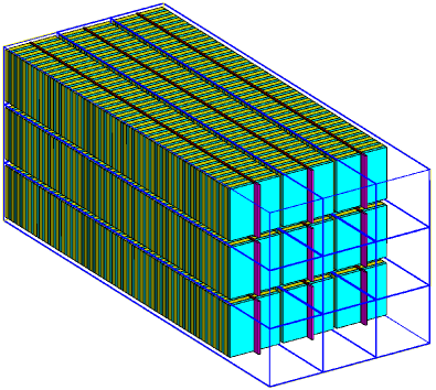
Figure 28: Geant4 representation of 9 calorimeter modules showing the WLS (in red) positioned vertically in the middle of the each module.

One of shortcomings of EJ-232 scintillator is the light absorption length (13.5 $\pm$ 0.5 cm) in the spectra range useful for exciting the EJ-299-27 WLS. To mitigate this problem the WLS will be positioned in the middle of the calorimeter module, as shown in Fig. 28, instead of along one side. The advantage of this design is that light travels half the length in the scintillator and is absorbed less. As a result. the light yield is increased by almost a factor of two. Another advantage is the resulting symmetric distribution of reconstructed particle position (a source of systematic error in angle reconstruction) and reduction of non-linearity of calorimeter response.

In simulation, the time of flight is found by analyzing the signal from the module with the most energy deposited. A flash ADC with sampling step of 2 ns (500 MHz) is simulated and the time is found when the signal reaches at 1/4 of its amplitude. With EJ-232 scintillator and EJ-299-27 WLS simulation predicts 0.65 ns RMS time resolution. Muon tests performed at JLab showed that simulation is able to predict muon time resolution with 5% precision. Based on this the predicted hadron time resolution is quite realistic.

2.8.4 Light Guides

Light guides are required to transport the light from the WLS to the PMT. Production of 288 or more adiabatic light guides based on a traditional twisted-strip design would take considerable time and resources. However, we are exploring the alternative light guide design shown in Fig. 29. This design is well-suited to injection molding techniques and, after extensive searchers, we have found companies that are capable of manufacturing acrylic light guide of this design with appropriate surface quality. The ability to produce the light guides with injection molding will greatly reduce the cost of production and gives additional design options, such as a lip to strengthen the scintillator/WLS glue joint, without significant increase in cost.

A Geant4 based simulation of the light guide has been developed to optimize light collection efficiency. The efficiency is estimated with and without aluminum foil wrapping. Without aluminum foil light collection efficiency is 65%, with aluminum foil wrapping (assuming 90% reflection) light collection efficiency is 75%.

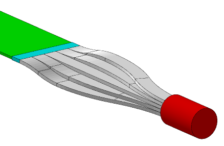
Figure 29: Light guide design from Geant4.

2.8.5 Phototubes

Simulation shows that the light produced and propagated in ELJEN-299-27 WLS has wavelength in the 410-500 nm range. Over 95% of photons have wavelength in 410-460 nm range. PMTs that have bi-alkali based cathodes are well suited to this photon spectrum range (they have max sensitivity around 420 nm). Since the XP2262-type PMTs from BigHAND detector have bi-alkali photo-cathodes, they can be coupled with ELJEN-299-27 and BC-484.

2.8.6 DAQ and Trigger

The energy from a single hadronic shower will be typically spread over 9 modules or more. To provide an effective trigger signal, the signals from groups of modules, corresponding to each possible hadronic shower location, must be summed prior to discrimination. This can be done using a complex system of linear fan-ins/fan-outs. However, we are also considering the use of low-resolution FADCS and executing the necessary summing and trigger logic using FPGAs.

2.8.7 Results of Component Tests

Oleg Gavrishchuk performed cosmic tests at JLab using one of the COMPASS modules provided by JINR, Dubna. The tests had the following goals: measure trigger time resolution of muons, estimate number of photo-electrons produced by minimum-ionizing particles (muons), and to calibrate and test our Geant4 simulation. The Geant4 comparison was done in the following steps:

• The number of photo-electrons found from cosmic muon passing across the module was inputted into the simulation (80 photo-electrons).

• Simulation was performed with muon going opposite to the light propagation direction and muons going in the direction of light propagation.

• The simulated timing results were compared with cosmic test results.

It was found that simulation and test results agree with good precision. With muons going in the direction of light propagation muon time resolution was 0.6 ns while, when going opposite to light propagation direction, the trigger time resolution was 0.77 ns. In both cases agreement of simulation with data was within 5%.

Cosmic tests with EJ-232 scintillator coupled with EJ-299-27 WLS were performed at CMU. The purpose of these tests were to study light attenuation length in the WLS, attenuation length in EJ-232 scintillator and to estimate the number of photo-electrons produced by coupling EJ-232 scintillator and EJ-299-27 WLS. Test results show that the attenuation length of light in the WLS is $\approx$ 1.5 m. The somewhat short attenuation length is not indicative of the optical quality of the WLS surface, but is a result of self absorption in the wavelength shifter and can not be avoided. The tests done in the lab were also simulated in Geant4 to estimate the accuracy of the simulation. Optical properties of the EJ-232 scintillator and EJ-299-27 wavelength shifter provided by ELJEN technology were input into the simulation. The simulation predicts 14 cm absorption length for EJ-232 scintillator, which is in good agreement with test results of 13.0 $\pm$ 0.5 cm. The mean number of photo-electrons produced by muons passing through the 0.635 cm thick EJ-232 scintillator is found to be 10 (light-guide efficiency is not taken account). The test setup is simulated in Geant4 and the scintillation yield per MeV of deposited energy is adjusted to match this result.

2.8.8 Plan and Summary

The overall geometric design of the calorimeter is complete; the only remaining issue is determining the optimal scintillator/WLS combination. The goal is to achieve good time resolution by using scintillators and wavelength shifters with relatively fast decay-times while, at the same, time, minimizing the reduction of light and spatial uniformity that will arise from short attenuation lengths.

The light guide simulation shows that we have a design that will give suitable light collection efficiency. Our plan is to produce these light guides using injection molding and our immediate goal is to obtain quotes from at least three companies for this project. If possible, we will obtain sample products from companies to provide a means of matching the surface properties obtained from injection molding to our Geant4 optical photon simulations.

Due to high cost of commercial scintillators ($\sim$$1M) new options for the scintillators are necessary. It appears that both Fermilab and JINR are able to produce scintillators with properties necessary for HCAL-J. We have written an MOU with Fermilab to produce scintillator samples with several concentration (0, 0.5, 1.0, 2.0, 3.0 percent) of PPO fluor. These samples will be tested at CMU to determine their absorption lengths and photon statistics. We expect additional samples to be provided by JINR in the near future. The results of these tests will be used in simulation to evaluate HCAL-J timing performance.

The final details of the HCAL-J design will be fixed when the tests of the prototype scintillator materials have been completed.

3 Summaries of Experimental Activities

3.1 E99-114 - Real Compton Scattering

Cross section measurement of $\pi^{0}$-photoproduction in RCS experiment

J. Annand, D. Hamilton, B. Wojtsekhowski

and the E99-114 Collaboration.

contributed by Johan Sjögren.

3.1.1 Overview of Experiment

The Real Compton Scattering experiment, E99-114, was designed to measure the Compton cross section, the polarization transfer in that reaction and the $\pi^{0}$-photoproduction cross section, all for wide angle scattering/photoproduction on the proton at multiple kinematic settings. The experiment ran in January and February 2002.

Liquid hydrogen was used as the target and photons were created through bremsstrahlung in a 6% Cu radiator. The left high resolution spectrometer detected the scattered proton, while the $e/\gamma$ was detected in an electromagnetic calorimeter. For the $\pi^{0}$ case one of the decay products($2\gamma$) was detected, primarily the forward boosted photon. The calorimeter[1] consisted of 704 blocks of lead glass and it was assembled specifically for the experiment. A deflection magnet was installed between the target and the calorimeter to slightly offset electrons allowing for a kinematical distinction between electrons and photons.

The experiment offers a test of constituent counting rules and pQCD predictions of the scaling of the cross sections. It is also possible to infer information about connected form factors. Likewise the polarization transfer is a good test of the predictions of pQCD and GPD techniques. Results for the Compton channel were published in 2005[2] and 2007[3].

3.1.2 Analysis update

The analysis is now focused on the $\pi^{0}$-channel, the remaining channel of interest. The $\pi^{0}$-channel was partially analyzed for background subtraction during the study of the Compton channel. This preliminary analysis is outlined in Ref. [4].

Since the experiment was performed while the ROOT-based Hall A analyzer code was still being developed the old analysis software is a mix of the FORTRAN based ESPACE and the early C++ analyzer. This has now been changed and the software has been updated/ported into the contemporary standard.

The calibration of the calorimeter is very important for accurate extraction of the $\pi^{0}$ yield. It was noted in the beginning of this year that the final calorimeter calibrations were in part missing, presumably lost in the abyss of time, and the existing parts were not sufficiently well made. Hence, the calibration is being remade aiming to improve timing, position- and energy-resolution. Figure 30 shows the improvements made for the energy resolution for a selected kinematic point. This kinematic point was chosen as an example due to the fact that the old calibration displayed both a constant offset and an unnecessarily large spread.

The goal of the calibration is to maximize visibility of the characteristic correlation between decay angle and energy for the photons originating from $\pi^{0}$ decay. By knowing the angle it is easy to calculate the expected energy of the photon. The difference between this calculated energy and the measured energy in the calorimeter should for $\pi^{0}$ events be a Gaussian distribution, see Fig. 31. This proves a solid identification of pion events.

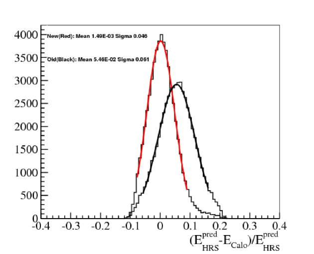
Figure 30: A comparison between the old energy reconstruction calibration and the remade one. $E_{HRS}^{pred}$ is the energy calculated from HRS variables assuming $ep$ scattering and $E_{Calo}$ is the energy measured by the calorimeter.

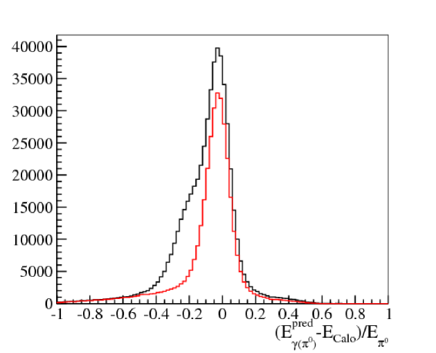
Figure 31: The energy difference, between the energy measured by the calorimeter $E_{Calo}$ and the expected photon energy $E_{\gamma(\pi^{0})}^{pred}$ calculated from the decay angle, as a fraction of the pion energy $E_{\pi^{0}}$. Red represents data with cuts to remove elastic electron events, black is without those cuts.

3.2 E04-007 - $\pi^{0}$

Precision Measurements of Electroproduction of $\pi^{0}$ near Threshold:
A Test of Chiral QCD Dynamics

J.R.M. Annand, D.W. Higinbotham, R. Lindgren, B. Moffit, B. Norum, V. Nelyubin, spokespersons,

M. Shabestari and K. Chirapatimol, students

and

The Hall A Collaboration.

contributed by Richard Lindgren and Cole Smith.

3.2.1 Introduction

The experiment is designed to measure the electroproduction reaction $p(e,e^{\prime}p)\pi^{0}$ of neutral pions off the proton at the lowest possible invariant mass W. Results from previous electroproduction measurements at Mainz with four-momentum transfers of $Q^{2}$ = 0.10 GeV/c² [1] and $Q^{2}$ = 0.05 GeV/c² [2] were in disagreement with the $Q^{2}$ dependence predicted by Heavy Baryon Chiral perturbation theory (HBChPT) and also inconsistent with the predictions of the MAID model [3]. If the Mainz discrepancies remain unresolved, they will constitute a serious threat to the viability of Chiral Dynamics as a useful theory of low energy pion production. Our experiment has measured absolute cross sections as precisely as possible from threshold to $\Delta W$ = 30 MeV above threshold at four-momentum transfers in the range from $Q^{2}$ = 0.050 GeV/c² to $Q^{2}$ = 0.150 GeV/c² in small steps of $\Delta Q^{2}$ = 0.01 GeV/c². This will cover and extend the Mainz kinematic range allowing a more sensitive test of chiral corrections to Low Energy Theorems for the S and P wave pion multipoles. In addition, the beam asymmetry was measured, which can be used to test predictions for the imaginary components of the of S wave $E_{0+}$ and $L_{0+}$ pion multipoles, which are sensitive to unitary corrections above the $n\pi^{+}$ threshold. Mainz recently repeated the electroproduction measurements and now report [4] that the new results are more consistent with HBChPT predictions, but are in disagreement with their own previous measurements [2]. In view of the importance of knowing whether or not HBChPT is valid in this domain, it is imperative that an independent set of measurements be reported.

3.2.2 Experimental Results

The experiment was performed using the Hall A Left High Resolution Spectrometer (LHRS) to detect the electron and the large acceptance BigBite spectrometer instrumented with MWDC followed by $E-\Delta E$ scintillation paddles to detect and identify the proton. A model independent partial wave analysis was made by fitting the measured cross section to a Legendre polynomial series assuming s and p-wave dominance. The total cross section $\sigma_{0}$ was extracted from the fit and is plotted as orange squares in Figure 1 as a function of $Q^{2}$= from 0.047 GeV² to 0.105 GeV² for $\Delta W$ = from 0.5 MeV to 11.5 MeV, which extends the kinematic range previously explored in threshold electroproduction. The size of the orange square data point is typical of the statistical error and excludes the systematic error at this time. The red curve is a HBChPT calculation using parameters taken from fitting the old Mainz $Q^{2}$=0.1 GeV/c² data [1]. The green curve and and the blue curves are calculations from the phenomenological models DMT and MAID07. The latest Mainz results below 4 MeV [4] shown as green points in Figure 1 are in agreement with our data. The HBChPT calculation [7] fits the trend of the data below $Q^{2}$= 0.10 GeV² from threshold up to about $\Delta W$ = 11.5 MeV. Above $Q^{2}$= 0.10 GeV² the HBChPT calculation increases linearly with $Q^{2}$ substantially departing from the data.

We are continuing to study improvements in the LHRS simulation to better understand our W resolution at threshold and the effects of target straggling and bin migration due to resolution smearing. We are also working to improve the VDC calibration and energy loss corrections in LHRS to achieve the best performance at threshold. In order to get a handle on our systematic errors associated with electron detection with the LHRS such as angular acceptance, momentum calibration, pointing, charge integration, detector efficiency, and absolute beam energy and energy drifts, single arm measurements were made on carbon and tantalum foils before and after every change in kinematics. The carbon foil was enriched to 99.95$\%$ ¹²C and was 83.88 mg/cm² in thickness. The angular distribution of elastic cross section measurements on carbon with moderately tight cuts on the vertical acceptance $\Delta\theta_{tg}$ is shown in Figure 2. The data are compared with DWBA phase-shift calculations [8] using an 18 term Fourier-Bessel charge density determined from fitting previous NIKHEF data [9] over a similar $Q^{2}$ range but at lower electron beam energies. The radiative corrected green data points were taken at an average beam energy of 1.192 GeV at angles of 12.5, 14.5, 16.5 and 20.5 degrees. The yellow points are the results of the DWBA calculation using a charge density fit to the NIKHEF data. A closer look at the small differences between our data and the calculation show that the differences average around 5$\%$ excluding the minimum where energy dependent dispersion effects may not be accounted for. This excellent agreement suggest that any systematic errors associated with the central region of the acceptance, dead time, charge integration, detector efficiencies, etc. are of the order of 5% or less on average.

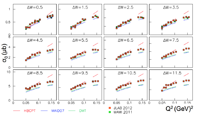
Figure 32: The total $p\pi^{0}$ C.M. cross section, $\sigma_{0}$($\mu$b), is plotted versus $Q^{2}$(GeV²). Each plot corresponds to an invariant mass bin $\Delta W$ measured in MeV relative to threshold. The orange points correspond to the JLAB 2012 data and the green points to the MAMI data points [4]. The red, green, and blue curves correspond to calculations of expected results from different models.

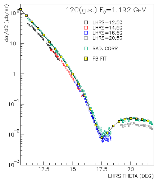
Figure 33: The elastic differential scattering cross section measurements and model calculations are plotted versus the LHRS Hall A spectrometer electron scattering angle. The black, red, blue, and gray points are absolute cross section measurements (uncorrected for radiation effects) after cuts on the vertical LHRS acceptance angle $\theta_{tg}$. The different colors represent the LHRS central angles of 12.5, 14.5, 16.5 and 20.5 degrees. The green points represent the radiation corrected measurements. The black curve and the yellow data points represent the DWBA calculation described in the text.

3.3 E05-015 - $A_{y}$ in ${}^{3}\mathrm{He}$(e,e’)

Measurement of the Target Single-Spin Asymmetry in Quasi-Elastic ³He${}^{\uparrow}(e,e^{\prime})$

T. Averett, J.-P. Chen and X. Jiang, spokespersons,

and

the Hall A Collaboration.

contributed by Y.-W. Zhang.

3.3.1 Motivation

In the past several years, nuclei and nucleon structures are often studied by measuring form factors using the Born approximation, which assumes one photon exchange neglecting the exchange of multiple photons. However, as new precision data on cross sections and polarization observables becomes available, the importance of two-photon exchange contributions cannot be ignored. For elastic scattering, $A_{y}$ is expected to be zero in the one-photon exchange approximation due to time-reversal invariance, but it can receive a non-zero contribution from the interference between the single-photon exchange amplitude and the imaginary part of the two-photon exchange amplitude. Although the importance of observing $A_{y}$ has been realized for many years, a non-vanishing $A_{y}$ has never been clearly established.

3.3.2 The experiment

JLab experiment E05-015 measured the neutron single spin asymmetry (SSA), $A_{y}^{n}$, formed by scattering unpolarized electrons from a polarized effective neutron target. The target polarization vector was normal to the electron scattering plane. The experiment used a longitudinally polarized electron beam at energies of 1.2, 2.4 and 3.6 GeV with an average current 12 $\mu$A. However, the polarized electron beam was summed over the two helicity states to achieve an unpolarized beam. The residual beam charge asymmetry was less than 100 ppm for a one-hour run.

The polarized target used in this experiment was a 40 cm long glass cell filled with 10.92 atm of ³He and a small amount (0.13 atm) of N₂ gas to reduce the depolarization effects. The target was polarized through spin-exchange optical pumping (SEOP) [1] of a Rb-K mixture. In order to reduce systematic uncertainty, the target polarization vector was automatically flipped every 20 minutes using adiabatic fast passage (AFP). The polarization was monitored during each spin-flip using nuclear magnetic resonance (NMR) measurements. Electron paramagnetic resonance (EPR) measurements were also used periodically throughout the experiment in order to calibrate the NMR signal. The target polarization during the experiment is shown in Fig. 34, an average in-beam target polarization of (51.4$\pm$0.4$\pm$2.9)$\%$ was achieved in this experiment.

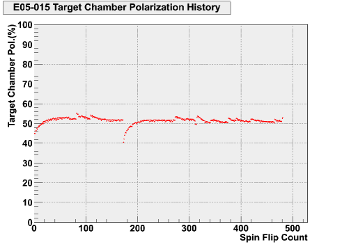
Figure 34: E05-015: ³He target performance during the experiment.

The beam passed through the glass cell and was rastered with a 3 mm $\times$ 3 mm pattern to reduce the possibility of local beam-induced density changes in the target. Scattered electrons from the target were observed using the two Hall A high resolution spectrometers (HRS) [2], left HRS at 17^∘ beam-left and right HRS at 17^∘ beam-right. Both spectrometers were configured to detect electrons in single-arm mode using nearly identical detector packages consisting of two dual-plane vertical drift chambers for tracking, two planes of segmented plastic scintillator for trigger formation, and a CO₂ gas Cherenkov detector and Pb-glass total-absorption shower counter for pion rejection. The left HRS and right HRS were synchronized during the experiment in order to increase the statistics and as a method to cross-check results. The kinematics settings during this experiment are provided in Table 3.

Table 3: Kinematics setting for the A_y measurements. Listed are the central four-momentum transfer, $\langle$Q${}^{2}\rangle$; beam energy, E₀; HRS central angle, $\theta$; the HRS central momentum, P₀.

$\langle$Q${}^{2}\rangle$(GeV${}^{2})$	E0(GeV)	$\theta$(∘)	P0(GeV/$c$)
0.13	1.245	17.0	1.176
0.46	2.425	17.0	2.181
0.96	3.605	17.0	3.086

3.3.3 Analysis progress

The raw experimental asymmetries were extracted as a function of energy transfer, $\omega$. For each data bin, they were formed as

$$A_{\mathrm{raw}}=\frac{Y^{\uparrow}-Y^{\downarrow}}{Y^{\uparrow}-Y^{\downarrow}}$$ (1)

where the electron yield, $Y^{\uparrow(\downarrow)}$, is the number of electrons, $N^{\uparrow(\downarrow)}$, in the target spin-up (spin-down) state that pass all the PID cuts, normalized by accumulated charge, $Q^{\uparrow(\downarrow)}$, and DAQ live-time, $LT^{\uparrow(\downarrow)}$:

$$Y^{\uparrow(\downarrow)}=\frac{N^{\uparrow(\downarrow)}}{Q^{\uparrow(\downarrow)}\cdot LT^{\uparrow(\downarrow)}}$$ (2)

The raw asymmetry was then corrected for nitrogen dilution and target polarization. The nitrogen dilution factor is defined as

$$f_{\mathrm{N_{2}}}\equiv\frac{\rho_{\mathrm{N_{2}}}\sigma_{\mathrm{N_{2}}}}{\rho_{\mathrm{{}^{3}He}}\sigma_{\mathrm{{}^{3}He}}+\rho_{\mathrm{N_{2}}}\sigma_{\mathrm{N_{2}}}}$$ (3)

where $\rho$ is the density and $\sigma$ is the unpolarized cross-section. The nitrogen density was measured when filling the target cell and the cross-section was determined experimentally by electrons elastically scattered from a reference cell filled with a known quantity of N₂. The denominator was taken from the production data.

3.3.4 Preliminary results

The physics asymmetry A${}_{y}^{\mathrm{{}^{3}He}}$ was finally obtained after corrections for radiative effects. Results for A${}_{y}^{\mathrm{{}^{3}He}}$ are shown in Fig. 35 for all three kinematic settings of the experiment and A${}_{y}^{\mathrm{{}^{3}He}}$ as a function of $\omega$ for all three kinematic settings of the experiment are shown in Fig. 36. The error bars on the data points are statistical only with the total experimental systematic error indicated as an error band. The systematic uncertainty in A${}_{y}^{\mathrm{{}^{3}He}}$ includes contributions from inconsistencies of LHRS and RHRS results, live-time asymmetry, target polarization, target misalignment, target density fluctuation, nitrogen dilution and radiative corrections.

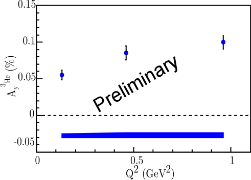
Figure 35: The vertical asymmetry of polarized ³He at $\langle$Q${}^{2}\rangle$=0.13, 0.46 and 0.96 GeV².

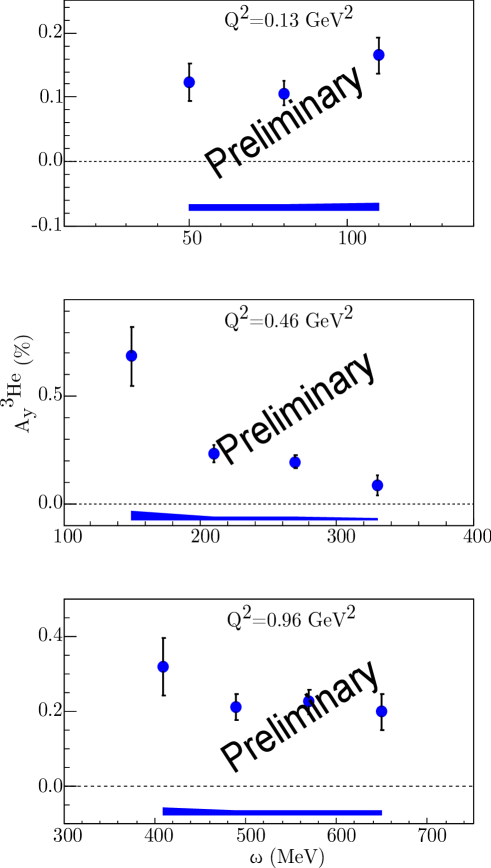
Figure 36: The vertical asymmetry of polarized ³He as a function of $\omega$ at $\langle$Q${}^{2}\rangle$=0.13, 0.46 and 0.96 GeV².

3.3.5 Remaining tasks

Two main tasks remain before publication. First the data must also be corrected for proton dilution if we are to show $A_{y}^{n}$ rather than $A_{y}^{\mathrm{{}^{3}He}}$. The neutron asymmetry, $A_{y}^{n}$, can be extracted from the ³He asymmetry using the effective polarization approximation, given by

$$A_{y}^{n}=\frac{1}{(1-f_{p})P_{n}}(A_{y}^{\mathrm{{}^{3}He}}-f_{p}P_{p}A_{y}^{p})$$ (4)

where the proton dilution factor $f_{p}=2\sigma_{p}/\sigma_{\mathrm{{}^{3}He}}$ . The effective neutron and proton polarizations in ³He are given by P_n=0.86${}_{-0.02}^{+0.036}$ and P_p=-0.028${}_{-0.004}^{+0.009}$ [3], respectively. If we know $f_{p}$ and $A_{y}^{p}$, we can extract $A_{y}^{n}$. Second, the systematic uncertainties budget must be finalized. Generating reliable estimates for most systematics will be straightforward for this experiment.

3.4 E05-102 - $A_{x}$, $A_{z}$ in ${}^{3}\mathrm{He}$(e,e’d)

Measurement of $A_{x}$ and $A_{z}$ asymmetries in the quasi-elastic ${}^{3}\overrightarrow{\mathrm{He}}$(e,e’d) reaction

S. Gilad, D.W. Higinbotham, W. Korsch, B.E. Norum, S. Širca spokespersons,

contributed by Miha Mihovilovic and Simon Širca.

The E05-102 experiment [1] is devoted to a detailed study of the ${}^{3}\vec{\mathrm{He}}(\vec{\mathrm{e}}\mathrm{e}^{\prime}\mathrm{d})$, ${}^{3}\vec{\mathrm{He}}(\vec{\mathrm{e}},\mathrm{e}^{\prime}\mathrm{p})\mathrm{d}$, ${}^{3}\vec{\mathrm{He}}(\vec{\mathrm{e}},\mathrm{e}^{\prime}\mathrm{p})\mathrm{pn}$ processes at low $Q^{2}$. The experiment in which double-polarization (beam-target) transverse and longitudinal asymmetries in these exclusive channels have been measured, has been performed in Summer 2009. Its main purpose is to approach the ground-state structure of the ${}^{3}\mathrm{He}$ nucleus by studying the missing-momentum ($p_{\mathrm{miss}}$) dependence of the asymmetries. These dependences are rather strong; in particular, it is seen that various components of the ${}^{3}\mathrm{He}$ ground-state wave-function have quite distinct signatures that become apparent only with a sufficient lever arm in $p_{\mathrm{miss}}$.

Theoretical input for acceptance averaging

The bulk of the detector calibrations has been performed, including the optics calibration of the BigBite spectrometer [2]. The data analysis is now at the stage when the theoretical results are being averaged over the experimental acceptance, and the largest progress has been made in the ${}^{3}\vec{\mathrm{He}}(\vec{\mathrm{e}},\mathrm{e}^{\prime}\mathrm{d})$ channel. We have received the results from the Bochum/Krakow group that span our whole accepted range of $p_{\mathrm{miss}}$ (discussed below), as well as preliminary results from the Hannover/Lisbon group which are currently being extended to a larger range of $p_{\mathrm{miss}}$. Since these calculations are extremely CPU-intensive, we rely on a $35$-point grid in the $(E^{\prime},\theta_{\mathrm{e}})$ plane to cover the complete acceptance. The grid corresponding to the data taken at $E=2425.5\,\mathrm{MeV}$ and $\theta_{\mathrm{e}}=12.5^{\circ}$ (central) is shown in Fig. 37.

Figure 37: Acceptance in $E^{\prime}$ versus $\theta_{\mathrm{e}}$ for $E=2425.5\,\mathrm{MeV}$ ($Q^{2}\approx 0.25$), with the mesh of $35$ kinematics points used in the averaging procedure.

Presently we are binning the theory in 25 $p_{\mathrm{miss}}$ bins ranging from $6\,\mathrm{MeV}/c$ to $294\,\mathrm{MeV}/c$ to ensure smooth averaging. The theoretical asymmetries are available only for the centers of each electron kinematics bin; due to the kinematic restrictions posed by energy and momentum conservation, it becomes physically impossible (in some bins) to find a corresponding calculated asymmetry for all $p_{\mathrm{miss}}$. On the other hand, real data span the whole bin and in general contain all missing momenta, even such that are forbidden at the exact center of the bin. To prevent such acceptance mismatches that could skew the resulting asymmetries, we consider only those data that lie within the missing-momentum range accessible by the theory.

By using the codes provided by the theorists we have generated — in each of the $35$ regions shown above — the asymmetries for each $p_{\mathrm{miss}}$ bin (or the corresponding $\theta_{dq}$, which is equivalent) as functions of $\phi_{dq}$. We use $25$ bins in $\phi_{dq}$ to cover the entire range between $0^{\circ}$ and $360^{\circ}$. This means that for each electron kinematics the asymmetries at $625$ different $(p_{\mathrm{miss}},\phi_{dq})$ points were determined.

Interpolation in $(p_{\mathrm{miss}},\phi_{dq})$

The asymmetries corresponding to intermediate values of $p_{\mathrm{miss}}$ and $\phi_{dq}$, where the asymmetries were not calculated, were then obtained by two-dimensional interpolation between these $625$ points. The same procedure was used for each of the $35$ electron kinematics. An example of the interpolated 2D asymmetry for electron kinematics #12 is shown in Fig. 38.

Figure 38: The theoretical asymmetry $A(\theta^{*}=73^{\circ},\phi^{*}=0^{\circ})$ as a function of $\phi_{dq}$ and $p_{\mathrm{miss}}$ obtained by interpolation between the values computed at $625$ different $(p_{\mathrm{miss}},\phi_{dq})$ points (kinematics #12).

Averaging the theoretical asymmetries

The averaging of the theoretical asymmetries over the kinematic acceptance of the electron spectrometer was then performed on an event-by-event basis. Each event was assigned to one of the $35$ possible boxes in the $(E^{\prime},\theta_{\mathrm{e}})$ plane shown in Fig. 37. Once the electron kinematics of an event was fixed, the measured values of $p_{\mathrm{miss}}$ and $\phi_{dq}$ were used to pick the corresponding value of the interpolated asymmetry. The obtained value was then stored in a histogram (see Fig. 39 (left)).

Figure 39: [Left] The distribution of events in terms of the predicted asymmetry $A(\theta^{*}=73^{\circ},\phi^{*}=0^{\circ})$ and $p_{\mathrm{miss}}$. [Right] Acceptance-averaged theoretical asymmetry as a function of $p_{\mathrm{miss}}$. The mean value of the asymmetry for each $p_{\mathrm{miss}}$ has been obtained by calculating the weighted average of the asymmetries in the 2D histogram in the corresponding $p_{\mathrm{miss}}$ bin.

The final acceptance-averaged theoretical asymmetries for each $p_{\mathrm{miss}}$ bin and their variation were then obtained by evaluating a weighted average of the contents of the 2D histogram (a sort of weighted projection on the $p_{\mathrm{miss}}$ axis). An example is shown in Fig. 39 (right). The error bars on the asymmetries are not a measure of the theoretical uncertainty. Rather, they reflect the scatter of data in any given $p_{\mathrm{miss}}$ bin: the population of the asymmetry is more condensed at low $p_{\mathrm{miss}}$ (red blob in the 2D histogram) while it spreads out widely at high $p_{\mathrm{miss}}$ (green and blue regions).

Work in progress

Apart from obtaining the results from further theory groups, we are presently striving to devise a smoother initial $(E^{\prime},\theta_{\mathrm{e}})$ configuration so that a multi-dimensional interpolation (not only in the hadron momenta and angles but also in the electron variables) would be possible, thus allowing us to exploit the full statistics.

Although the E05-102 experiment was dedicated to a precision measurement of the asymmetries, we have also been working on the extraction of the absolute cross-sections. This requires a rather intricate simultaneous use of MCEEP and the existing theory results on the discrete grid, which is work in progress. We are also trying to incorporate both proton knock-out channels, ${}^{3}\vec{\mathrm{He}}(\vec{\mathrm{e}},\mathrm{e}^{\prime}\mathrm{p})\mathrm{d}$ and ${}^{3}\vec{\mathrm{He}}(\vec{\mathrm{e}},\mathrm{e}^{\prime}\mathrm{p})\mathrm{pn}$, since the beam energy was too high for a clean separation of the two-body and three-body breakup channels.

3.5 E06-002 - PREX

PREx: Precision Measurements of the Neutron Radius of Lead

K.S. Kumar, R.W. Michaels, P.A. Souder, G.M. Urcioli, spokespersons,

and

the PREX Collaboration.

contributed by Seamus Riordan.

The PREX experiment completed in Spring 2010 with the purpose of measuring the RMS neutron radius of lead through the use of parity-violating electron scattering. The results for this were published in early 2012 [1] and showed the existence of a neutron skin with a 95% confidence level for the first time. Plans to improve the precision on this measurement to $0.06~{}\mathrm{fm}$ have been approved for after the 12 GeV upgrade [2].

The main parity-violating neutron radius results were presented in the previous annual report. In the time since then, additional analysis has been performed on separate, ancillary measurements which are non-parity violating in nature and required to constrain the systematic error involving possible transverse asymmetry components. This component, $A^{m}_{n}$, is described by

$$A^{m}_{n}=A_{n}\vec{P}_{e}\cdot\hat{k}$$ (5)

where $A_{n}$ is the maximal value of the asymmetry, $\vec{P}_{e}$ is the electron polarization vector, and $\hat{k}$ is the vector normal to the electron scattering plane.

Such components are introduced if the beam is not entirely longitudinally polarized. Because this asymmetry is non-parity violating, it is in principle different from the desired measured quantity and could also become fairly large. To minimize the effects from this, running the two high resolution spectrometers in Hall A in a symmetric configuration cancels out the azimuthal modulation given in Eq. 5. However, even with this, it is necessary to perform direct measurements to provide a constraint on the size of the systematic effect.

The value of the transverse asymmetry is interesting by itself. Due to time reversal symmetry, in the single photon exchange approximation it is identically zero, meaning that this becomes a probe of multi-photon exchanges. Understanding such effects is crucial particularly in the study of nucleon form factors and are notoriously difficult to calculate due to the presence of the off-shell propagator in the multiphoton exchange diagrams. Additionally, in doing such calculations, effects such as coulomb distortions must also be taken into account for nuclei of high $Z$.

Results from the PREX experiment and previous HAPPEX measurements were recently published for a variety of nuclei [3]. It was observed that for three light nuclei, $\mathrm{H}$, ${}^{4}\mathrm{He}$, and ${}^{12}\mathrm{C}$ that the results were in good agreement with predictions using a dispersion relation approach [4]. However, for similar measurements on ${}^{208}\mathrm{Pb}$ there is a severe discrepancy, and the asymmetry was observed to be compatible with zero, Fig. 40. At present there is no definitive explanation for such an effect, though the calculations of [4] do not include Coulomb distortions which grow rapidly with $Z$ and are critical in understanding the elastic parity-violating asymmetry on ${}^{208}\mathrm{Pb}$.

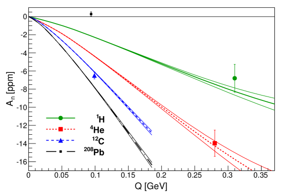
Figure 40: Transverse asymmetry results from both the PREX and HAPPEX experiments on four different nuclei.

3.6 E06-014 - $d_{2}^{n}$

A Precision Measurement of $d_{2}^{n}$: Probing the Lorentz Color Force

S. Choi, X. Jiang, Z.-E. Meziani, B. Sawatzky, spokespersons,

and

the $d_{2}^{n}$ and Hall A Collaborations.

Contributed by D. Flay, D. Parno and M. Posik.

3.6.1 Physics Motivation

3.6.1.1 $d_{2}^{n}$: Quark-Gluon Correlations in the Nucleon

To date, extensive work has been done investigating the spin structure function $g_{1}$ within the context of the Feynman parton model and pQCD. However, far less is known about the $g_{2}$ structure function. It is known to contain quark-gluon correlations. It follows from a spin-flip Compton amplitude and may be written as

$$g_{2}\left(x,Q^{2}\right)=g_{2}^{WW}\left(x,Q^{2}\right)+\bar{g}_{2}\left(x,Q^{2}\right),$$ (6)

where $g_{2}^{WW}$ is the Wandzura-Wilczek term, which may be expressed entirely in terms of $g_{1}$ [1]

$$g_{2}^{WW}\left(x,Q^{2}\right)=-g_{1}\left(x,Q^{2}\right)+\int_{x}^{1}\frac{g_{1}\left(y,Q^{2}\right)}{y}dy.$$ (7)

The second term is given as

$$\bar{g}_{2}\left(x,Q^{2}\right)=-\int_{x}^{1}\frac{1}{y}\frac{\partial}{\partial y}\left[\frac{m_{q}}{M}h_{T}\left(y,Q^{2}\right)+\xi\left(y,Q^{2}\right)\right]dy,$$ (8)

where $h_{T}$ is the transverse polarization density, and $\xi$ is a term arising from quark-gluon correlations. Here, $h_{T}$ is suppressed by the ratio of the quark mass $m_{q}$ to the target mass $M$. Therefore, a measurement of $\bar{g}_{2}$ provides access to quark-gluon interactions inside the nucleon [2]. ⁢

Additionally, a measurement of both $g_{1}$ and $g_{2}$ allows for the determination of the quantity $d_{2}^{n}$, which is formed as the second moment of a linear combination of $g_{1}$ and $g_{2}$

$$d_{2}^{n}\left(Q^{2}\right)=\int_{0}^{1}x^{2}\left[2g_{1}^{n}\left(x,Q^{2}\right)+3g_{2}^{n}\left(x,Q^{2}\right)\right]dx=3\int_{0}^{1}x^{2}\bar{g}_{2}^{n}\left(x,Q^{2}\right)dx.$$ (9)

$d_{2}^{n}$ also appears as a matrix element of a twist-3 operator in the operator product expansion [3]

$$\langle P,S\mid\bar{\psi}_{q}\left(0\right)gG^{+y}\left(0\right){\gamma}^{+}\psi_{q}\left(0\right)\mid P,S\rangle=2MP^{+}P^{+}S^{x}d_{2}^{n},$$ (10)

where $G^{+y}=\frac{1}{\sqrt{2}}\left(B^{x}-E^{y}\right)$. We see from Equations 8–10 that $d_{2}^{n}$ is a twist-3 matrix element that measures quark-gluon interactions.

Recent work has shown [4, 5] that at high $Q^{2}$, $d_{2}^{n}$ is seen as a color Lorentz force averaged over the volume of the nucleon. This is given by the expression of the transverse (color) force on the active quark immediately following its interaction with a virtual photon

$$F^{y}\left(0\right)\equiv-\frac{\sqrt{2}}{2P^{+}}\langle P,S\mid\bar{\psi}_{q}\left(0\right)gG^{+y}\left(0\right){\gamma}^{+}\psi_{q}\left(0\right)\mid P,S\rangle=-\frac{1}{2}M^{2}d_{2}^{n}.$$ (11)

This theoretical interpretation reveals how $g_{2}$ and subsequently $d_{2}^{n}$ will allow us to examine the color interactions of the constituents inside the nucleon.

While bag and soliton model calculations of $d_{2}$ for the neutron yield numerical values consistent with those of lattice QCD, current experimental data differs by roughly two standard deviations (see the highest $Q^{2}$ data in Figure 41). One of the goals of our experiment is to improve the experimental error on the value of $d_{2}^{n}$ by a factor of four. It subsequently provides a benchmark test of lattice QCD calculations, shown in Figure 41.

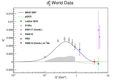
Figure 41: $\text{d}_{\text{2}}^{\text{n}}$ as a function of $Q^{2}$. All the data shown with the exception of the SLAC E155x data are dominated by resonance contributions. E06-014 data will observe mostly the deep inelastic scattering (DIS) contribution. The projected error on from E06-014 [6] is shown, along with the lattice QCD result [7]. The dashed green curve shows the pQCD evolution from the lattice point [8] based on the calculations of [9, 10]. Data from JLab experiments E94-010 [11] and RSS [12] are included in the plot. For comparison to the resonance contribution, a MAID model [13] is plotted. Also plotted is the total $d_{2}$ from SLAC experiment E155x [14].

3.6.1.2 $A_{1}$: The Virtual Photon-Nucleon Asymmetry

Another quantity of interest is the virtual photon-nucleon longitudinal spin asymmetry $A_{1}$. It provides insight into the quark structure of the nucleon and can be defined as

$$A_{1}\left(x,Q^{2}\right)\equiv\frac{\sigma_{1/2}-\sigma_{3/2}}{\sigma_{1/2}+\sigma_{3/2}},$$ (12)

where the subscript 1/2 (3/2) gives the projection of the total spin of the virtual photon-nucleon system along the virtual photon direction corresponding to the nucleon’s spin anti-parallel (parallel) to the virtual photon. Constituent quark models (CQM) and pQCD models predict $A_{1}$ to be large and positive at large $x$. Figure 42(a) shows the current world data compared to these models. It is seen that the CQM (yellow band [15]) describes the trend of the data reasonably well. The pQCD parameterization with hadron helicity conservation (dark blue curve [20])—assuming quark orbital angular momentum to be zero—does not describe the data well. However, the pQCD model allowing for quark orbital angular momentum to be non-zero (green curve [21]) describes the data well, pointing perhaps to the importance of quark orbital angular momentum in the spin structure of the nucleon.

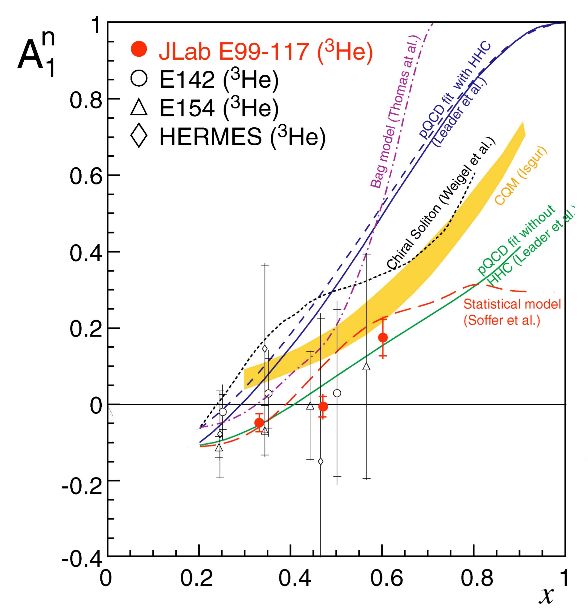
(a) $A_{1}^{n}$

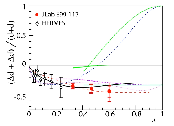
(b) $\Delta d/d$

Figure 42: Current data for $A_{1}^{n}$ and $\Delta d/d$. (42(a)): The current world data for the neutron $A_{1}$ from SLAC E143 [16] and E154 [17] and HERMES [18], along with JLab E99-117 [19]. Also shown are CQM models and various pQCD models; (42(b)): the corresponding models and data from HERMES and JLab for $\Delta d/d$.

Combining $A_{1}^{n}$ data measured on a polarized effective neutron target with $A_{1}^{p}$ data measured on a polarized proton target allows access to $\Delta u/u$ and $\Delta d/d$. Recent results from Hall A [19] and from CLAS [22] showed a significant deviation of $\Delta d/d$ from the pQCD predictions, which have that ratio approaching 1 in the limit of $x\rightarrow 1$ (Fig. 42(b)). As part of the 12 GeV program, two approved experiments (one in Hall A [23] and one in Hall C [24]) will extend the accuracy and $x$ range of this measurement, but a measurement of $A_{1}^{n}$ at the kinematics of this experiment (E06-014) will provide valuable support (or refutation) of prior JLab results, while producing additional input for theoretical models in advance of the coming experiments at 12 GeV.

3.6.2 The Experiment

The experiment ran in Hall A of Jefferson Lab from February to March of 2009, with two beam energies of $E=4.73$ and $5.89$ GeV, covering the resonance and deep inelastic valence quark regions, characterized by $0.2\leq x\leq 0.7$ and $2\textrm{ GeV}^{2}\leq Q^{2}\leq 6$ $\textrm{GeV}^{2}$. The coverage in the $x$ and $Q^{2}$ plane is shown in Figure 43. ⁢

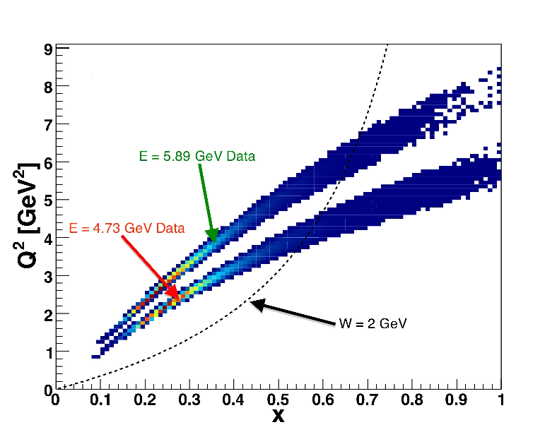
Figure 43: The E06-014 kinematic coverage in $Q^{2}$ and $x$. The lower band is the 4.73 GeV data set and the upper band is the 5.89 GeV data set. The black dashed line shows W = 2 GeV. The data to the left and right of this line corresponds to DIS and resonance data, respectively.

In order to calculate $d_{2}^{n}$, we scattered a longitudinally polarized electron beam off of a ³He target, in two polarization configurations – longitudinal and transverse. ³He serves as an effective polarized neutron target since roughly $86\%$ of the polarization is carried by the neutron. This is due to the two protons in the nucleus being primarily bound in a spin singlet state [25, 26]. ⁢

We measured the unpolarized total cross section $\sigma_{0}$ and the asymmetries $A_{\parallel}$ and $A_{\perp}$. The cross section was measured by the Left High-Resolution Spectrometer (LHRS), while the asymmetries were measured by the BigBite Spectrometer. The LHRS and BigBite were oriented at scattering angles of $\theta=45^{\circ}$ to the left and right of the beamline, respectively. ⁢

Expressing the structure functions entirely in terms of these experimental quantities, we have the expression for $d_{2}^{n}$

$$d_{2}^{n}=\int_{0}^{1}\frac{MQ^{2}}{4{\alpha}^{2}}\frac{x^{2}y^{2}}{\left(1-y\right)\left(2-y\right)}{\sigma}_{0}\left[\left(3\frac{1+\left(1-y\right)\cos\theta}{\left(1-y\right)\sin\theta}+\frac{4}{y}\tan\left(\theta/2\right)\right)A_{\perp}+\left(\frac{4}{y}-3\right)A_{\parallel}\right]dx,$$ (13)

where $x=Q^{2}/2M\nu$, $\nu=E-E^{\prime}$ is the energy transfer to the target, $E^{\prime}$ is the scattered electron energy, and $y=\nu/E$ is the fractional energy transfer to the target. The asymmetries are given by

$$A_{\parallel}=\frac{N^{\downarrow\Uparrow}-N^{\uparrow\Uparrow}}{N^{\downarrow\Uparrow}+N^{\uparrow\Uparrow}}\quad\textrm{and}\quad A_{\perp}=\frac{N^{\downarrow\Rightarrow}-N^{\uparrow\Rightarrow}}{N^{\downarrow\Rightarrow}+N^{\uparrow\Rightarrow}},$$

where $N$ is the number of electron counts measured for a given configuration of beam helicity (single arrows) and target spin direction (double-arrows).

While $d_{2}^{n}$ was the main focus of the experiment, the measurement of the asymmetries allowed for the extraction of $A_{1}^{n}$, according to

$$A_{1}^{n}=\frac{1}{D\left(1+\eta\xi\right)}A_{\parallel}^{n}-\frac{\eta}{d\left(1+\eta\xi\right)}A_{\perp}^{n},$$ (14)

where $D$, $\eta$, $\xi$ and $d$ are kinematic factors [27].

3.6.3 Beam Polarization

E06-014 used a polarized electron beam at energies of 4.73 and 5.89 GeV. The polarization of the electron beam was measured independently through Compton and Møller scattering. During the running of E06-014, there were several Møller measurements performed while Compton measurements were taken continuously throughout the experiment. Figure 44 shows the beam polarization as a function of BigBite run number for the Møller and Compton results. The beam polarization data was split into four run sets and the average polarization for each run period was then computed by taking into account both the Compton and Møller data. The final beam polarizations can be seen in Table 4 [28].

Run Set	Beam Energy (GeV)	$P_{e}$ from Compton	$P_{e}$ from Møller	Combined $P_{e}$
1	5.90	$0.726\pm 0.018$	$0.745\pm 0.015$	$0.737\pm 0.012$
2	4.74	$0.210\pm 0.011$	-	$0.210\pm 0.011$
3	5.90	$0.787\pm 0.020$	$0.797\pm 0.016$	$0.793\pm 0.012$
4	4.74	$0.623\pm 0.016$	$0.628\pm 0.012$	$0.626\pm 0.010$

Table 4: Final beam polarization for E06-014, corrected for beam fluctuations. For run set 2 there was no Møller measurement.  [28]

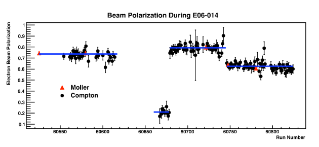
Figure 44: Final electron beam polarization from Møller and Compton measurements for E06-014. Note there was no Møller measurement for the second run set [28].

3.6.4 ³He Target Density

A complete understanding of the target density is essential, since the calculation of the target polarization from the EPR and NMR measurements depends on the ³He density. The number density of ³He was measured in both the pumping and the target chambers. This measurement was achieved by exploiting the fact that collisions with ³He atoms broaden the D1 and D2 absorption lines of rubidium [29]. The ³He number density at room temperature, $n_{0}$, can be obtained by measuring the width of the D1 and D2 absorption lines and subtracting a 1% N₂ contribution.

The full analysis to determine the ³He density may be found in [31].

3.6.5 Polarized ³He Target

Knowledge of the target polarization is crucial when performing a double-spin asymmetry experiment. E06-014 used the standard Hall A polarized ³He target with two holding field directions: longitudinal and transverse in plane, with respect to the electron beam direction. The target polarization was extracted through electron paramagnetic resonance (EPR). The longitudinal polarization was cross checked using nuclear magnetic resonance (NMR) measurements. EPR measurements were taken every several days during the experiment, while NMR measurements were taken every few hours.

3.6.5.1 EPR Calibration

The frequency shift of potassium level transitions in the presence of ³He was measured using EPR. This frequency shift $\Delta\nu_{EPR}$ can be related to the target polarization, $P_{{}^{3}\mathrm{He}}$

$$\Delta\nu_{EPR}=\frac{4\mu_{0}}{3}\frac{d\nu_{EPR}}{dB}\kappa_{0}\mu_{{}^{3}\mathrm{He}}n_{pc}P_{{}^{3}\mathrm{He}},$$ (15)

where $\mu_{0}$ is the vacuum permeability; $\mu_{{}^{3}\mathrm{He}}$ is the magnetic moment; $\frac{d\nu_{EPR}}{dB}$ is the derivative of the EPR frequency with respect to the magnetic field; $\kappa_{0}$ is the enhancement factor, and $n_{pc}$ is the pumping chamber number density. EPR measurements give the absolute ³He polarization in the pumping chamber. However, it is the ³He polarization in the target cell that needs to be extracted. A polarization gradient model is used in order to determine the polarization between the two chambers. The change in polarization in the two chambers is given by

$$\frac{dP_{T}}{dt}=d_{P}\left(P_{T}-P_{P}\right)+\gamma_{SE}\left(P_{Rb}-P_{P}\right)-\Gamma_{P}P_{P},$$ (16)

$$\frac{dP_{P}}{dt}=d_{T}\left(P_{P}-P_{T}\right)+\Gamma_{T}P_{T},$$ (17)

where $P_{T,P,Rb}$ is the polarization of the target chamber, pumping chamber ³He and rubidium atoms. $\Gamma_{T}$ is the depolarization rate of the ³He; $\gamma_{SE}$ is the spin exchange rate between ³He and rubidium atoms, and $d_{P,T}$ are diffusion constants that depend on the target cell geometries and ³He density. Taking the equilibrium solution, we obtain an expression that relates the polarizations between the two chambers

$$P_{T}=\frac{1}{1+\frac{\Gamma_{T}}{d_{T}}}P_{P}.$$ (18)

The calculated diffusion constant, $d_{T}$, is shown in Table 5 for both target spin directions. The depolarization rate is a sum of various depolarization rates caused by different sources as shown in Equation 19. $\Gamma^{He}+\Gamma^{wall}$ are determined by measuring the target cell polarization live time. The depolarization rate due to the beam, $\Gamma^{beam}$, was found by using a model [30]. $\Gamma^{\nabla B}$ was calculated by measuring the gradient magnetic holding fields which polarize the target, and were found to be negligible. $\Gamma^{AFP}$ was also found to be negligible. Table 6 shows the results of the depolarization rates.

$$\Gamma_{T}=\Gamma^{He}+\Gamma^{wall}+\Gamma^{beam}+\Gamma^{AFP}+\Gamma^{\nabla B}$$ (19)

Table 5: $d_{T}$ diffusion constant for both target spin directions.

Parameter	Target Spin	Value	Units	Uncertainty [%]
$d_{T}$	Long.	0.892	hour-1	15.04
$d_{T}$	Trans.	0.889	hour-1	15.06

Table 6: List of parameters used to calculate $\Gamma_{T}$

Parameter	Value	Units	Uncertainty [%]
$\Gamma^{He}+\Gamma^{wall}$	0.0714	hour-1	35
$\Gamma^{beam}$	0.0794	hour-1	10.45
$\Gamma^{AFP}$	neg.	hour-1	neg.
$\Gamma^{\nabla B}$	neg.	hour-1	neg.
$\Gamma_{T}$	0.1508	hour-1	36.53

During EPR measurements, a NMR measurement was done simultaneously, allowing us to calibrate NMR measurements during production with the EPR measurements by taking the ratio of the target polarization measured by EPR, $P_{T}$, and the measured NMR amplitude, $h$. A conversion factor $c^{\prime}$ can then be formed that allows NMR measurements to be converted into an absolute ³He polarization.

After applying the $c^{\prime}$ factor to all NMR measurements, a linear interpolation was done as a function of run time. This allowed the extraction of a target polarization on a run-by-run basis. The pumping and target chamber polarizations were extracted via EPR measurements, shown in Figure 45.

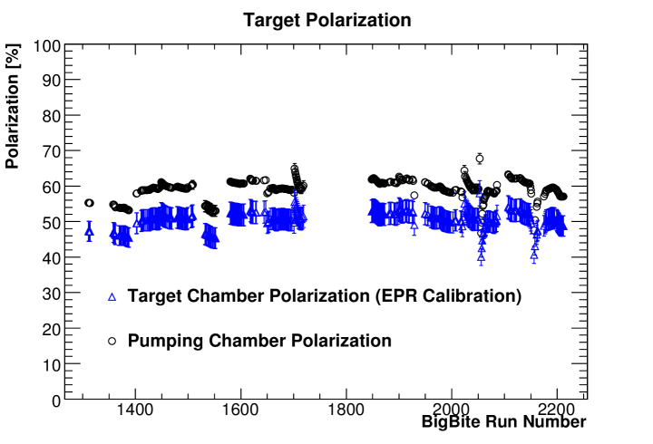
Figure 45: ³He polarization in the pumping and target chambers. Some ³He polarization is lost while traveling between the two chambers.

3.6.5.2 Water Calibration

In addition to calibrating the NMR using EPR measurements, NMR measurements on a water sample can also be used to calibrate ³He NMR signals. The polarization of the protons in the water, when placed in a known magnetic field, can be solved exactly. The water polarization was measured by performing NMR measurements on a target cell filled with water. The water target cell was similar in geometry to the ³He filled cells. The water NMR signal was detected in two sets of pick-up coils that extended the length of the target (40 cm) on both sides. A NMR cross-calibration factor needs to be applied when using the water calibration, because the NMR measurement for the water cell and ³He target cell took place in two different locations and the signals were measured in two different pick-up coil sets. The cross-calibration factor can be calculated by selecting a ³He target spin direction and then taking the ratio of the ³He NMR signal measured in the pick-up coils at the water cell position and the ³He NMR signal measured at the ³He target cell position during a production run. This could in principle be done for all target spin directions, longitudinal and transverse. Unfortunately, there was no transverse NMR measurements with the ³He in the water cell position; as a result, there is a large systematic uncertainty on the transverse target polarization. With this in mind, the water calibration for the longitudinal direction is used to cross-check the target polarization extracted from the longitudinal EPR calibration.

Due to the fact that the polarization of water is small ($\approx 7\times 10^{-9}$), a water polarization model was used in order to fit the water NMR signal and accurately extract the NMR signal height. The time evolution of the water polarization can be described by the Bloch equations given as

$$\frac{dP_{x}(t)}{dt} = -\frac{1}{T_{2}}P_{x}(t)+\gamma\left(H(t)-H_{0}\right)P_{y}(t)+\frac{1}{T_{2}}\chi H_{1},$$ (20)

$$\frac{dP_{y}(t)}{dt} = -\gamma\left(H(t)-H_{0}\right)P_{x}(t)-\frac{1}{T_{2}}P_{y}(t)+\gamma H_{1}P_{z}(t),$$ (21)

$$\frac{dP_{z}(t)}{dt} = -\gamma H_{1}P_{y}(t)-\frac{1}{T_{1}}P_{z}(t)+\frac{1}{T_{1}}\chi H(t),$$ (22)

where $P$ is the water polarization in a particular direction; $t$ is the time; $T_{1}$ and $T_{2}$ are the longitudinal and transverse spin relaxation times; $H_{0}$ is the resonance field; $H_{1}$ is the transverse field component; $H(t)=H_{0}+\alpha t$ is the field component along the z-axis; $\alpha=1.2$ G/s is the field sweep speed; $\gamma$ is the gyro-magnetic ratio of the proton; $\chi=\frac{\mu_{p,H_{2}O}}{k_{B}T}$, with $\mu_{p,H_{2}O}$ being the magnetic moment of a proton in water; $k_{B}$ is the Boltzmann constant and $T$ is the target chamber temperature.

Using the Bloch equations, an effective polarization, $P_{\mathit{eff}}=\sqrt{P_{x}^{2}+P_{y}^{2}+P_{z}^{2}}$, can be calculated and leads to the integral equation shown in Equation 23. This equation was solved numerically using Mathematica. However, an analytic function is needed to fit the water NMR signal, so approximations to $P_{\mathit{eff}}$ were made. Figure 46 shows the water NMR fit results for 6,189 NMR sweeps.

$$\centering P_{\mathit{eff}}(t)=e^{-(t-t_{i})/T_{1}}\left[P_{eq}(t_{i})+\frac{1}{T_{1}}\int_{t_{i}}^{t}e^{(u-t_{i})/T_{1}}P_{eq}(u)du\right]\@add@centering$$ (23)

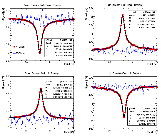
Figure 46: Presented are the sweep up and sweep down signals for the downstream and upstream coils. The Y lock-in channel is shown as red markers with water fit shown as a black line. The X lock-in channel is shown as a blue line.

While the geometries of the water and ³He cells are similar, they are not identical. To correct for this discrepancy, the ratio of the magnetic flux through the ³He and water cells was calculated. With this information, a water calibration constant can be formed, shown in Equation 24.

$$c_{w}=\left(\frac{P_{w}}{S_{w}}\right)\left(\frac{G_{w}}{G_{He}}\right)\left(\frac{\mu_{p}}{\mu_{He}}\right)\left(\frac{n_{p}\Phi_{w}}{n_{He}^{pc}\phi_{He}^{pc}+n_{He}^{tc}\phi_{He}^{tc}}\right)\left(\frac{S^{He}_{pick-up}}{S^{He}_{prod.}}\right),$$ (24)

where $w(p)$ means water target (proton), $He$ means ³He target, $P$ is the polarization, $S$ is the NMR signal height and $\mu$ is the magnetic moment. $S_{pick-up}$ is the NMR signal with the ³He target measured at the pick-up coil location where the water NMR was done. $S_{prod.}$ is the NMR signal measured with the ³He in the production position. Applying this constant to the interpolated NMR measurements, a run-by-run ³He target polarization can be extracted. By comparing the longitudinal target polarizations extracted from the EPR and water calibrations, both methods were found to give consistent results.

3.6.6 The Left High-Resolution Spectrometer

3.6.6.1 Unpolarized Total Cross Sections

The Left High-Resolution Spectrometer (LHRS) was used to measure the unpolarized total cross section. The analysis for the extraction of the experimental cross section, $\sigma_{\textrm{rad}}$, for the E = 4.73 GeV and 5.89 GeV data sets is shown in [31].

3.6.6.2 Radiative Corrections

Electrons lose energy due to interactions with material. This includes the material before and after the target, and the target material itself. These interactions will alter the electron’s true incident energy and also its true scattered energy. This ultimately results in a different cross section than the true value. These effects are characterized by ionization (or Landau straggling) and bremsstrahlung. There are also higher-order processes at the interaction vertex that must be considered. Collectively, the correction of these effects is called radiative corrections.

A first correction that must be done before carrying out the radiative corrections is to subtract the elastic radiative tail, since it affects all states of higher invariant mass $W$ [32]. For these kinematics, the elastic tail is negligible and was not subtracted from the data.

The ³He quasi-elastic tail, however, has a larger contribution and needs to be subtracted. The tail was built up from calculating the elastic tail of the proton and neutron using ROSETAIL [33] and adding them together as $2p+n$, to account for two protons and one neutron in ³He. The systematic effect of the subtraction on the resulting cross section, $\sigma_{\textrm{rad}}$, was $\leq$ 0.5%.

In considering the effects mentioned above, the measured cross section is realized in terms of a triple-integral

$$\sigma_{\textrm{rad}}\left(E_{s},E_{p}\right)=\int_{0}^{T}\frac{dt}{T}\int_{E_{s}^{min}}^{E_{s}}dE_{s}^{\prime}\int_{E_{p}}^{E_{p}^{max}}dE_{p}^{\prime}I\left(E_{s},E_{s}^{\prime},t\right)\sigma_{r}\left(E_{s}^{\prime},E_{p}^{\prime}\right)I\left(E_{p},E_{p}^{\prime},T-t\right),$$ (25)

where $\sigma_{\textrm{rad}}$ is the measured (radiated) cross section, $\sigma_{r}$ is the internally-radiated cross section. $E_{s}$ is the incident electron energy, $E_{p}$ is the scattered electron energy. $I\left(E_{0},E,t\right)$ is the probability of finding an electron with incident energy $E_{0}$ that has undergone bremsstrahlung with final energy $E$ at a depth $t$ inside a material [32, 34].

In order to unfold the Born cross section, an iterative procedure is carried out in RADCOR [35]. It amounts to an “energy-peaking” approximation, resulting in the calculation of

$$\sigma_{b}^{i}=\frac{1}{\textrm{C}}\left[\sigma_{\textrm{rad}}-\int\left(\ldots\right)\sigma_{b}^{i-1}dE_{s}^{\prime}-\int\left(\ldots\right)\sigma_{b}^{i-1}dE_{p}^{\prime}\right],$$ (26)

where C and the two integrals are defined in Equation IV.2 in [32]. $\sigma_{b}^{i}$ is the Born cross section obtained for the $i^{\textrm{th}}$ iteration of the code, $\sigma_{\textrm{rad}}$ is the radiated cross section to be corrected. $\sigma_{b}^{i}$ is then re-inserted into equation for the next iteration. It was found that the calculation converges within the first 3–4 iterations. Figure 47 shows the preliminary Born cross sections.

In E06-014, we took data for only two $E_{s}$ values of 4.73 GeV and 5.89 GeV. However, we need enough data to properly calculate the integrals above. Therefore, we used a suitable cross section model [36] to fill in the rest of the phase space for each data set.

(a) E = 4.73 GeV

(b) E = 5.89 GeV

Figure 47: Preliminary results for the unpolarized Born cross sections, compared to P. Bosted and V. Mamyan’s F1F209 model [36] for E $=$ 4.73 GeV (47(a)) and 5.89 GeV (47(b)). The error bars show the statistical errors, while the bands show the in quadrature sum of systematic errors from experimental cuts, radiative corrections and other uncertainties (Sect. 3.6.6.3), and errors due to the subtraction of background signals from nitrogen scattering and positron production in scattering from ³He. The systematic errors and radiative corrections are still tentative.

3.6.6.3 Systematic Errors

Table 7 shows the systematic errors determined from the data as compared to the projected errors in the E06-014 proposal [6]. One large contribution comes from the cuts on the target variables; the cut on the horizontal scattering angle, $\phi$, contributes at the $\sim$ 2% level. This is not surprising since the Mott cross section is most sensitive to this quantity. Another large contribution comes from the radiative corrections. The source of this is due to the dependence on the cross section model used and how accurately we know the material thicknesses in the electron’s path before and after scattering. These two radiative correction errors combine for an error of $<$ 4%.

The largest contribution to the systematic errors comes from the uncertainty in subtracting the background signals in scattering from nitrogen and pair production in scattering from ³He. The presence of nitrogen in the cell is to prevent depolarization effects on ³He [29]. The largest error from the background signals comes from the positrons, contributing at a level of $\approx$ 0.8 nb/GeV/sr at the lowest bin in $E_{p}$. These errors are still tentative. Adding these contributions in quadrature with the values listed in Table 7 gives the error bands shown in Figure 47.

Type	Proposal (%)	Experiment (%)
PID Efficiency	$\approx$ 1	1
Background Rejection Efficiency	$\approx$ 1	1
Beam Charge	$<$ 1	$\approx$ 0.3
Acceptance Cut	2–3	2.7
Target Density	2–3	2.2
Dead Time	$<$ 1	$<$ 1
Radiative Corrections	$\leq$ 10	$<4$

Table 7: The systematic errors on the Born cross section compared to the estimates from the proposal. The largest contributions here come from the radiative corrections and the target cuts. However, all values are within the limits specified in the proposal.

3.6.7 The BigBite Spectrometer

3.6.7.1 The Double-Spin Asymmetries

The BigBite spectrometer was used to measure the parallel and perpendicular double-spin asymmetries between longitudinally polarized electrons and a longitudinally or transversely polarized ³He target. These asymmetries were then corrected for imperfect beam and target polarizations. Corrections were also made for dilution effects due to the presence of $\textrm{N}_{2}$ in the target [29]. The full details of this analysis may be found in [31].

3.6.7.2 Positron Contamination Correction

In addition to $\textrm{N}_{2}$ contamination, pair-produced electrons from $\pi^{0}$ and $\gamma$ decay can also contaminate the asymmetry. This is treated as a dilution to the electron asymmetry, and is corrected for by applying a dilution factor $D$:

$$A_{\textrm{c}}^{e^{-}} = \frac{1}{D}A_{\textrm{m}}^{e^{-}}$$ (27)

$$D = 1-\frac{N_{e^{+}}}{N_{e^{-}}}$$ (28)

where $A_{\textrm{c}}^{e^{-}}$ is the corrected electron asymmetry; $A_{\textrm{m}}^{e^{-}}$ is the electron asymmetry with target and beam dilution corrections, but no positron dilution corrections; $N_{e^{+}}/N_{e^{-}}$ is the positron to electron ratio, measured using BigBite. With BigBite in negative polarity, electrons bend up into the detector, whereas positrons bend downwards.

After applying this correction to the parallel and perpendicular asymmetries, we obtain the values shown in Figure 48(a) for E = 4.73 GeV and Figure 48(b) for E = 5.89 GeV. Radiative corrections have not been applied. Work is ongoing to determine the pair-produced electron asymmetry and its effect on the desired electron asymmetry.

(a) E = 4.73 GeV

(b) E = 5.89 GeV

Figure 48: Physics asymmetries with positron corrections. The magenta line shows the DIS threshold, below which is the DIS region. The error bars represent the statistical errors. No radiative corrections. The positron corrections have not been finalized. (48(a)): E = 4.73 GeV data; (48(b)): E = 5.89 GeV data.

3.6.8 Preliminary Physics Results

In this section, we present our preliminary physics results for asymmetry $A_{1}^{{}^{3}\textrm{He}}$ and the spin structure functions $g_{1}$ and $g_{2}$ on ³He. These results are preliminary because work is being done on the radiative corrections to the asymmetries along with a Geant4 simulation to further investigate the difference between the bend-up and bend-down acceptances in the BigBite spectrometer. Work concerning the corrections to the asymmetries due to asymmetry of pair-produced electrons is also ongoing.

The extraction of $d_{2}^{{}^{\textrm{3}}\textrm{He}}$ and $\text{d}_{\text{2}}^{\text{n}}$ along with the neutron asymmetry $A_{1}^{n}$, and the spin structure functions $g_{1,2}$ are also underway; however, the extraction is model-dependent. Previous experiments [19] have used Bissey et al.’s complete model in the DIS regime [39]. However, E06-014’s data spans both the DIS and resonance regions. A consistent treatment of both DIS and resonance data requires careful consideration of structure-function smearing [40]. We are working with W. Melnitchouk to extract neutron quantities across our entire kinematic range.

3.6.8.1 The Virtual Photon-Nucleon Asymmetry

Figure 49(a) and Figure 49(b) shows the preliminary result for $A_{1}^{{}^{3}\textrm{He}}$ at E = 4.73 and 5.89 GeV, respectively. Also shown is world data from SLAC E142 [37] and JLab E01-012 [38] and E99-117 [19]. The red (blue) data points indicate the DIS (resonance) data for this experiment. No radiative corrections have been applied to these data. The data from this experiment are consistent with the world data across a wide range in $x$, despite the larger error bars in the resonance region.

(a) E = 4.73 GeV

(b) E = 5.89 GeV

Figure 49: $A_{1}^{{}^{3}\textrm{He}}$ compared to the world data from SLAC E142 [37] and JLab E01-012 [38] and E99-117 [19]. The error bars on our data are statistical only. The radiative corrections to our data have not been applied, and the positron corrections are still under investigation. (49(a)): E = 4.73 GeV data; (49(b)): E = 5.89 GeV data.

3.6.8.2 The Spin Structure Functions

En route to extracting $d_{2}^{n}$, the spin structure functions $g_{1}$ and $g_{2}$ can be obtained according to:

$$g_{1} = \frac{MQ^{2}}{4{\alpha}^{2}}\frac{2y}{\left(1-y\right)\left(2-y\right)}\sigma_{0}\left[A_{\parallel}+\tan\left(\theta/2\right)A_{\perp}\right]$$ (29)

$$g_{2} = \frac{MQ^{2}}{4{\alpha}^{2}}\frac{y^{2}}{\left(1-y\right)\left(2-y\right)}\sigma_{0}\left[-A_{\parallel}+\frac{1+\left(1-y\right)\cos\theta}{\left(1-y\right)\sin\theta}A_{\perp}\right],$$ (30)

where $M$ is the nucleon mass; $\alpha$ is the electromagnetic fine structure constant; $y=\nu/E$, the fractional energy transfer to the target; $\theta$ is the electron scattering angle; $\sigma_{0}$ is the unpolarized total cross section; $A_{\parallel}$ ($A_{\perp}$) is the parallel (perpendicular) double-spin electron asymmetry.

The preliminary results for $g_{1}$${}^{{}^{\textrm{3}}\text{He}}$ and $g_{2}$${}^{{}^{\textrm{3}}\text{He}}$ are shown in Figure 50, which compares the data to various models [41, 42, 43, 44] and the world data. Radiative corrections have been applied only to the unpolarized total cross sections for the data from this experiment.

(a) $g_{1}$${}^{{}^{\textrm{3}}\textrm{He}}$ at E = 4.73 GeV

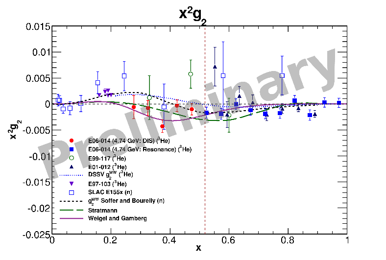
(b) $g_{2}$${}^{{}^{\textrm{3}}\textrm{He}}$ at E = 4.73 GeV

(c) $g_{1}$${}^{{}^{\textrm{3}}\textrm{He}}$ at E = 5.98 GeV

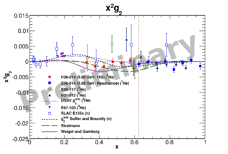
(d) $g_{2}$${}^{{}^{\textrm{3}}\textrm{He}}$ at E = 5.98 GeV

Figure 50: Preliminary results for the spin structure functions $g_{1}$ and $g_{2}$ on a ³He target for E = 4.73 and 5.89 GeV compared to the world data [14, 19, 37, 38, 45] and the DSSV model [41] and models from Weigel and Gamberg [42], Bourelly and Soffer [43], and Stratmann [44]. The error bars on our data are statistical only. The radiative corrections to our data have only been applied to the cross sections and not the asymmetries. The positron corrections to the asymmetries are still under investigation. (50(a)) and (50(b)): $g_{1}$${}^{{}^{\textrm{3}}\textrm{He}}$ and $g_{2}$${}^{{}^{\textrm{3}}\textrm{He}}$ for a beam energy of E = 4.73 GeV. (50(c)) and (50(d)): $g_{1}$${}^{{}^{\textrm{3}}\textrm{He}}$ and $g_{2}$${}^{{}^{\textrm{3}}\textrm{He}}$ for a beam energy of E = 5.89 GeV.

3.7 E07-006 - Short Range Correlations

Triple Coincidence ⁴He(e,e’pn) Measurements

S. Gilad, D. Higinbotham, V. Sulkosky, and J. Watson spokespersons,

and

the Hall A Collaboration.

contributed by I. Korover and N. Muangma.

Experiment E07-006 [1] was conducted to continue the study of nucleon-nucleon (NN) short-range correlations (SRC). During the first high luminosity triple coincidence experiment at JLab, E01-015 [2], we measured the $\left(\mathrm{e,e^{\prime}pp}\right)$ and $\left(\mathrm{e,e^{\prime}pn}\right)$ reactions on ¹²C over the $\left(\mathrm{e,e^{\prime}p}\right)$ missing momentum range from 275 to 550 MeV/$c$. These measurements were sensitive to the short-range NN tensor force. The recently completed triple coincidence experiment measured these reactions on ⁴He over the missing momentum range from 400 to 875 MeV/$c$ in order to study the short-range repulsive part of the NN interaction and investigate the transition from a tensor-force-dominated region. The kinematic conditions $\left(Q^{2}=2~{}\mathrm{GeV}^{2}\hskip 2.84544pt\mathrm{and}\hskip 2.84544ptx_{B}>1\right)$ allow us to extract the abundance of $pn$- and $pp$-correlated pairs with minimal interference from final state interactions, meson exchange currents and resonance production.

During the experimental run period, the detection of the neutrons in the triple coincidence ⁴He(e,e’pn) measurement was done by using the Hall A Neutron Detector (HAND), and the protons in the ⁴He(e,e’pp) measurement were detected in the BigBite hadron spectrometer [3]. The analysis so far has focused on calibration of the two high resolution spectrometers (HRSs), the neutron detector and the BigBite spectrometer. However, these calibrations are nearing completion, and preliminary results will soon be available.

3.7.1 ⁴He(e,e’p) Coincidence Time

The experiment requires good timing information from the HRSs. During the production measurement, the left HRS detected the scattered electron and provides the reference time. The relative time between the left HRS and right HRS is used to identify the recoil neutrons or protons in the third arm (HAND / BigBite), which are in coincidence with (e,e’p) events. These are the recoil particles from the breakup of pn-SRC/pp-SRC pairs respectively. The coincidence time distribution between the HRSs for one of the three kinematics is shown in Fig. 51 with a resolution of 0.6 ns. The same resolution is observed in the other two kinematical setups.

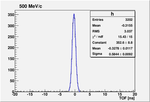
Figure 51: Coincidence time between the HRSs at 500 MeV/c

The first steps in the analysis of the (e,e’pn) events were

1. The time calibration of HAND.

2. The determination of the absolute neutron detection efficiency.

3.7.2 Time calibration of HAND

HAND consists of 112 (1-m long, 10-cm thick) scintillator bars arranged in 6 layers and an additional front layer of 64 thin (2 cm) counters that were used as a veto. In the first part of the timing calibration, time alignment between all bars was performed. We used the H(e,e’p) reaction to calibrate HAND in which electrons were detected by the left HRS and the protons in the neutron detector, located at 15 m from the target. Figure 52 shows the difference between the measured TOF and the calculated one based on the known proton momentum. As can be seen, the achieved resolution is $\sigma\approx$ 0.5 ns.

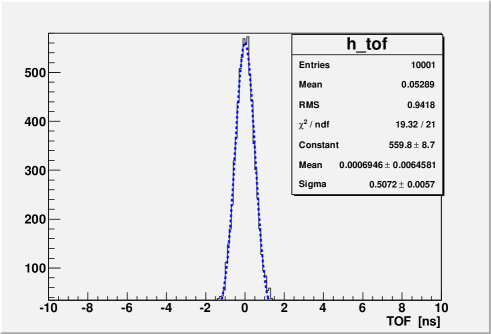
Figure 52: TOF for protons from the ⁴He(e,e’p) reaction as measured by the 30 detectors in the first layer of HAND.

The calibration procedure adjusts the relative timing between the different bars. The absolute timing and the TOF resolution was determined using the liquid deuterium target measuring the d(e,e’pn) exclusive reaction. The electron and proton were measured by the HRSs and the known momentum of the neutron by HAND. The difference between the measured TOF and that calculated based on the neutron known momentum is shown in Fig. 53. The resolution is $\sigma\approx$ 1.7 ns.

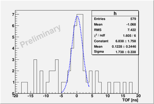
Figure 53: The difference between the Neutron TOF measured and calculated, see text for details.

3.7.3 Neutron detection efficiency

The absolute neutron detection efficiency was determined using the exclusive d(e,e’pn) reaction at two different kinematical settings corresponding to neutrons with mean momenta of 250 MeV/$c$ and 450 MeV/$c$. The measured efficiency compared to a simulation [4] is shown in Fig 54.

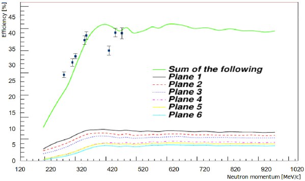
Figure 54: Neutron detection efficiency as a function of the neutron momentum, measured and simulated.

Following the calibration, the TOF spectrum for the 750 MeV/$c$ missing momentum is shown in Fig 55.

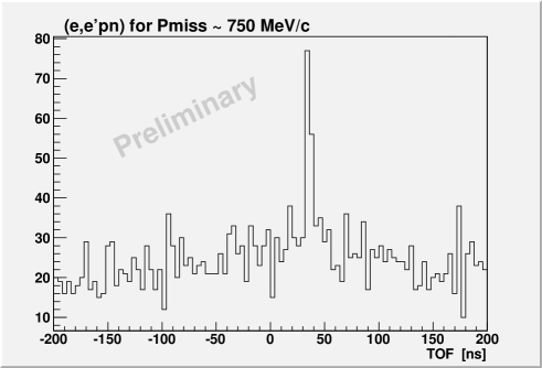
Figure 55: Neutron TOF distribution for the (e,e’p) missing momentum of 750 MeV/$c$.

A clear coincidence peak on top of random coincidence background can be identified at all of the measured missing momenta. The background level can be estimated by fitting to a constant background in the off-time region and also by using an event mixing procedure. The event mixing is done by taking the (e,e’p) information from one event and the neutron information from another event. The accepted events pass all the physical cuts. The angular correlation between the initial proton and the recoil neutron is shown in Fig 56. A clear back-to-back angular correlation of the short range np - pair can be seen above the background.

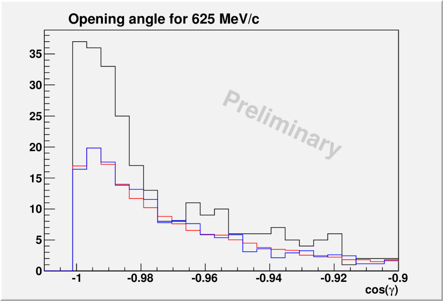
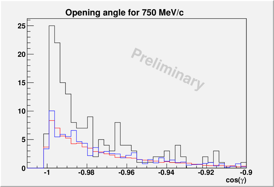
Figure 56: Cosine of the opening angle between the proton and the neutron. Black: Signal + Background, Blue: Background estimated by event mixing, Red: Background from the off time region.

3.7.4 BigBite Spectrometer Calibrations

The BigBite Spectrometer is used to detect the recoil proton partners. The BigBite Spectrometer consists of a single dipole, two Multi-Wire Drift Chambers (MWDCs), and two scintillator planes, named the dE and E planes. The Particle Identification (PID) process requires the clear separation of protons from deuterons and Minimum Ionizing Particles (MIPs). The momentum is calibrated against $\left|\vec{q}\right|$ from the left HRS using the elastic hydrogen data for the momentum range of 300–500 MeV/$c$. After a first iteration of calibrations, the resolution ($\sigma$) is 7.7 MeV/$c$, providing a better than 2% momentum resolution. The coincidence time between the left HRS (electron arm) and BigBite is used to eliminate backgrounds including random coincidence events as shown in Fig. 57 with an achieved resolution $<$ 1.4 ns.

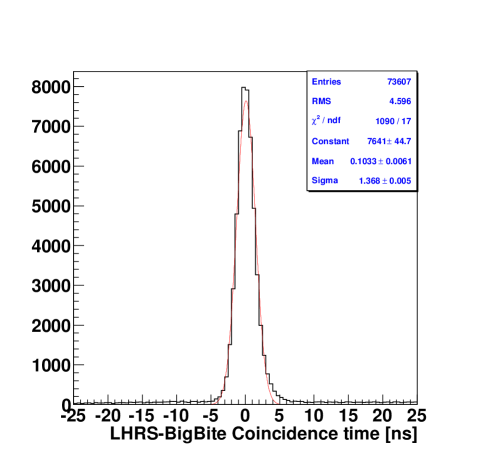
Figure 57: The coincidence time between the left HRS and BigBite for the elastic d(e,e’p) data. The red curve shows a fit to the data.

Different methods can be utilized via some combination of the energy deposited in the dE/E planes, the reconstructed momentum, and the coincidence time between the left HRS and BigBite. For the first method, the energy deposited in the dE plane vs. the energy deposited in E plane is shown in Fig. 58 for an elastic deuterium run.

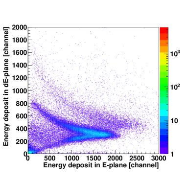
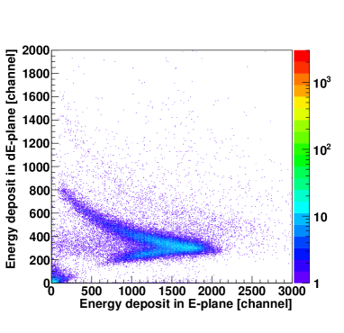
Figure 58: Energy deposited in the dE plane versus the energy deposited in the E plane. The left panel is without a timing cut on the left HRS and BigBite coincidence time, whereas the right panel is with a coincidence time cut on Fig. 57 to remove deuterons.

This method separates well the protons and deuterons from the MIPs but cannot separate the proton from the deuterons at high energy. By adding a coincidence time cut on the data, most of the deuterons can be removed as shown in the right-side panel of Fig. 58.

In the second method, the momentum vs. the energy deposited in each scintillator plane can also be used to separate different particle species as illustrated in Fig. 59.

Figure 59: The left panel shows the reconstructed BigBite momentum from the MWDC vs. the energy deposited in the dE plane. The right panel shows the reconstructed BigBite momentum vs. the energy deposited in the E plane.

This method shows the distinction of the proton strip from the deuteron strip, and there is a cleaner separation for the dE plane.

3.7.5 Summary

At this point, the analysis is focused on extraction of the cross section ratios of ⁴He(e,e’pn) to ⁴He(e,e’pp). This ratio was found in the 300 – 500 MeV/c missing momenta range to be about 18:1 [2]. As the missing momentum increases, the dominance of the tensor force is expected to be reduced and the short range repulsive force is expected to be more important, making the (e,e’pn)/(e,e’pp) ratio smaller. The measured ratio of the ⁴He(e,e’pn) to the ⁴He(e,e’pp) can hopefully teach us about the interplay between the tensor and the repulsive part of the short distance nucleon-nucleon force.

3.8 E07-007, E08-025 - DVCS

Deeply Virtual Compton Scattering

P. Bertin, C. Muñoz Camacho, A. Camsonne, C. Hyde, M. Mazouz, J. Roche, spokespersons,

and

the Hall A Collaboration.

contributed by C. Hyde.

3.8.1 Introduction

Generalized Parton Distributions (GPDs) describe the transverse spatial distribution of quarks and gluons inside a hadron, as a function of the longitudinal momentum fraction of the the parton. Deeply virtual Compton scattering ($ep\rightarrow ep\gamma$) is the simplest reaction (at least from the point of view of QCD theory) in which to study GPDs. To lowest order in QED, the exclusive electroproduction reaction is described by the coherent superposition of the virtual Compton scattering (VCS) and Bethe-Heitler amplitudes. The deeply virtual limit is defined as high $Q^{2}$, high $W^{2}$, but small net invariant momentum transfer $-t$ to the target proton. In this generalization of the Bjorken limit of Deep Inelastic Scattering (DIS), the virtual Compton amplitude simplifies to a power series in $1/Q^{2}$, with the leading ’Twist-2’ term determined by the GPDs.

Our Hall A DVCS program is focussed on the measurement of precision cross sections as a function of $Q^{2}$, at fixed $x_{\rm Bj}$ and $t$ [2]. This allows us to isolate the Twist-2 GPD terms from the higher order terms. In Oct–Dec 2010, we completed data taking for two DVCS experiments in Hall A: proton DVCS E07-007, and D$(e,e^{\prime}\gamma)pn$ E08-025. In these experiments, we measured the $(e,e^{\prime}\gamma)$ and $(e,e^{\prime}\pi^{0})$ reactions as a function of $t$ at a fixed $x_{\rm Bj}=0.36$, at three values of $Q^{2}$ and at two incident beam energies for each $Q^{2}$. The main goal of these experiments is to isolate the $|DVCS|^{2}$ and $\Re{\rm e}[DVCS^{\dagger}BH]$ terms in the cross section. This is possible, because the kinematic pre-factors of these two terms vary with the incident energy ($k$), with the ratio $\left|DVCS\right|^{2}:\Re{\rm e}\left[DVCS^{\dagger}BH\right]\sim k.$ This is a generalized Rosenbluth separation. A secondary goal of the experiment is to perform a Rosenbluth separation of $\sigma_{L}$ and $\sigma_{T}$ in the exclusive $N(e,e^{\prime}\pi^{0})N$ channels. This will help to clarify the role of the recently discovered transversity GPDs [1].

3.8.2 Analysis

In these two experiments, we detected the scattered electron in the HRS-L, and the emitted $\gamma$-ray in a dedicated calorimeter of 208 PbF₂ crystals. The $\gamma$-ray shower in the 208 element PbF₂ calorimeter is digitized by a custom 1 GHz analog sampling circuit based on the ANTARES ARS chip [3]. Sample single pulse and double pulse fits are displayed in Fig. 60. The $(e,e^{\prime}\gamma)$ coincidence timing, after all corrections, is displayed in Fig. 61. The PbF₂ energy response is calibrated with dedicated elastic H$(e,e_{\rm calo}p_{\rm HRS})$ runs. The resulting H$(e,e^{\prime}\gamma)X$ missing mass-squared spectrum is displayed in Fig. 62. Note that accidental coincidences and the background of H$(e,e^{\prime}\gamma)\gamma X^{\prime}$ events (where the two photons come from a neutral pion have not yet been subtracted. A simulation of the latter is in progress, based on the measured sub-sample of H$(e,e\pi^{0})X^{\prime}$ events in which the $\pi^{0}\rightarrow\gamma\gamma$ decay is fully reconstructed in the calorimeter.

The mass distribution of $\gamma\gamma$ events is displayed in the left-hand plot of Fig. 63. Events in the $\pi^{0}$ peak are used to fine-tune the calorimeter calibration. The result can be seen in the missing mass squared distribution of H$(e,e^{\prime}\pi^{0})$X events of the right hand plot of Fig. 63.

All calibrations for E07-007 and E08-025 are now complete.

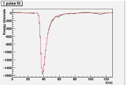
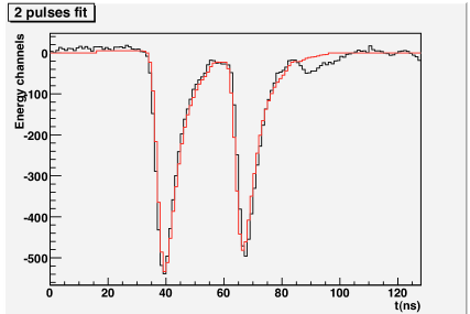
Figure 60: Sample 1 GHz waveforms for $\gamma$ shower in one crystal of PbF₂ calorimeter. Left: Single pulse fit; Right: Double pulse fit. Roughly $8\%$ of all events have at least one crystal with a double pulse signal.

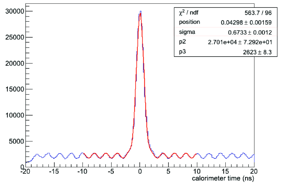
Figure 61: Coincidence time spectrum for $(e,e^{\prime}\gamma)$ events The $\gamma$ signal is a weighted sum of all PbF₂ crystals in the shower. The electron timing is corrected for time-walk in the HRS scintillator paddles, path length in the spectrometer, and other effects. The one-$\sigma$ timing resolution is 0.7 ns, the 2 ns beam structure is clearly visible. Within a $\pm 3$ ns coincidence window, the accidental to true coincidence ratio is $3\%$. All calorimeter signals of more than 0.1 GeV are included in this spectrum.

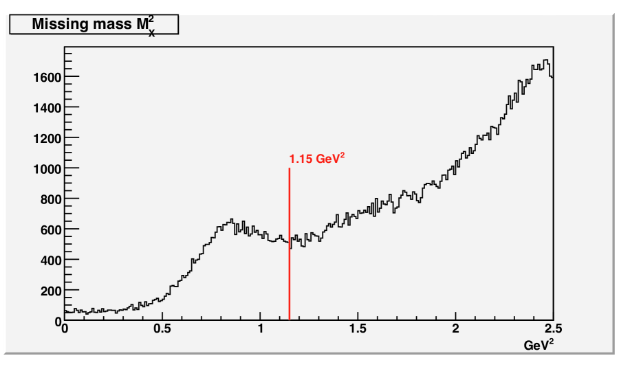
Figure 62: Missing mass squared $M_{X}^{2}$ distribution of H$(e,e^{\prime}\gamma)X$ events. The exclusive peak is at $M_{X}^{2}=M_{p}^{2}=0.88$ GeV². The hadronic H$(e,e^{\prime}\gamma)N\pi$ continuum starts at $M_{X}^{2}=(M_{p}+m_{\pi}^{0})^{2}=1.15$ GeV². Accidental coincidences and the statistical sample of H$(e,e^{\prime}\gamma)\gamma X^{\prime}$ events are not yet subtracted.

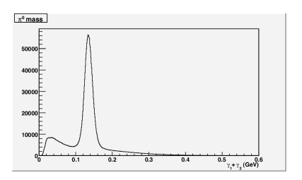
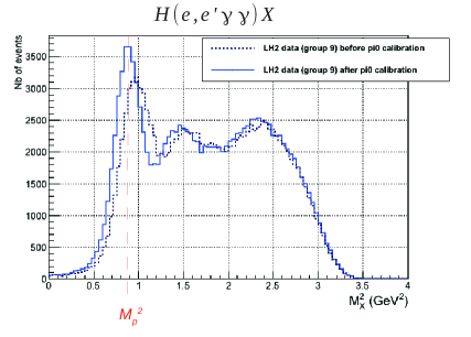
Figure 63: Left: ${\gamma\gamma}$ mass spectrum of H$(e,e^{\prime}\gamma\gamma)X$ events. The 1-$\sigma$ width of the $\pi^{0}$ peak is 11 MeV. Right: Missing mass squared $M_{X}^{2}$ of H$(e,e^{\prime}\pi^{0})X$ events before(dotted) and after (solid) refining the calorimeter calibrations based on the $\pi^{0}$ mass reconstruction.

3.9 E05-102, E08-005 - $A_{T}$, $A_{L}$, $A_{y}^{0}$ in ³He($e,e^{\prime}n$)

Measurements of the Double-Spin Asymmetries $A_{T}$ and $A_{L}$ and the Target Single-Spin Asymmetry $A_{y}^{0}$ in the Quasi-Elastic ³He^↑($e,e^{\prime}n$) Reaction

S. Gilad, D.W. Higinbotham, W. Korsch, B.E. Norum, S. Širca, E05-102 spokespersons,

T. Averett, D. Higinbotham, V. Sulkosky, E08-005 spokespersons,

and

the Hall A Collaboration.

contributed by E. Long (Kent State University).

3.9.1 Progress of ³He($e,e^{\prime}n$) Asymmetries

Progress has been made on the ${}^{3}\vec{\mathrm{He}}$($\vec{e},e^{\prime}n$) double-spin asymmetries for experiment E05-102, where the target was polarized in the transverse direction and longitudinal directions. The $A_{T}$ and $A_{L}$ observables are correlated to neutron electromagnetic form factors.

Data from the RHRS were used to isolate the quasi-elastic peak and apply basic kinematic cuts. It was also used to identify scattered electrons. Neutrons were identified using the Hall A Neutron Detector. The raw asymmetries for $A_{T}$ and $A_{L}$ are presented against the energy transfer, $\nu$, in Figures 64 and 65, respectively. Each asymmetry was measured at $Q^{2}$ values of 0.51 (GeV/$c)^{2}$ and 0.95 (GeV/$c)^{2}$.

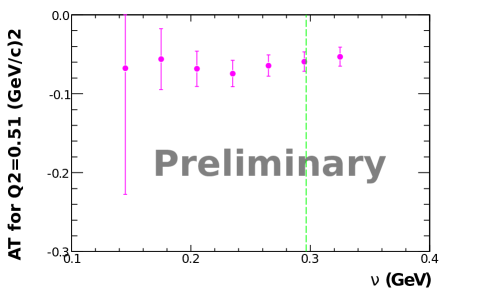
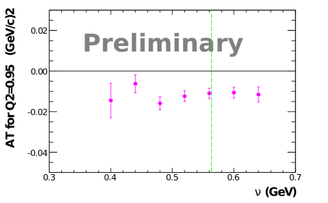
Figure 64: The raw asymmetry for $A_{T}$ against the energy-transfer $\nu$ is presented at $Q^{2}=0.505$(GeV/$c)^{2}$ on the left and at $Q^{2}=0.953$(GeV/$c)^{2}$ on the right. The green dashed line corresponds to the quasi-elastic peak.

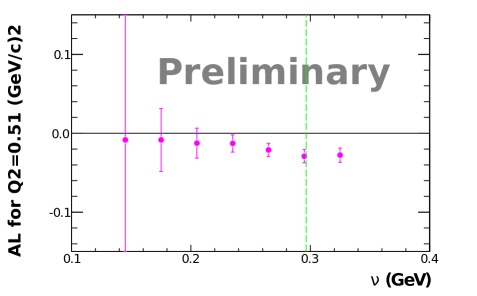
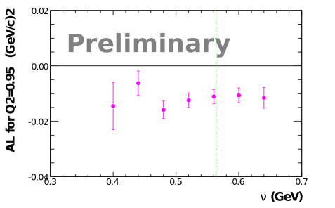
Figure 65: The raw asymmetry for $A_{L}$ against the energy-transfer $\nu$ is presented at $Q^{2}=0.505$(GeV/$c)^{2}$ on the left and at $Q^{2}=0.953$(GeV/$c)^{2}$ on the right. The green dashed line corresponds to the quasi-elastic peak.

In addition, a similar method was used to determine the target single-spin ³He^↑($e,e^{\prime}n$) asymmetry $A_{y}^{0}$, which ran using the same experimental set-up as E05-102 but with the target polarized in the vertical direction. The A_y observable is sensitive to final state interactions (FSI) and meson exchange currents (MEC). At low Q², contributions from FSI and MEC are expected to be large and decrease as Q² increases. Asymmetry measurements on the quasi-elastic peak were taken at $Q^{2}$ values of 0.13 (GeV/$c)^{2}$, 0.46 (GeV/$c)^{2}$, and 0.95 (GeV/$c)^{2}$. The raw asymmetry measurements are presented in Figure 66.

Dilution contributions from target polarization, beam polarization, neutron contamination, and nitrogen admixture in the target are in the process of being finalized for each of the asymmetries mentioned above. These factors will approximately double the magnitude of the raw asymmetries presented.

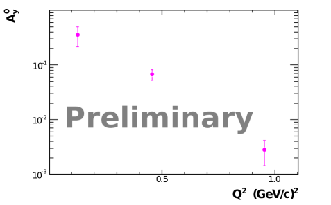
Figure 66: The raw asymmetry for $A_{y}^{0}$ against $Q^{2}$ is presented on a logarithmic scale.

3.10 E08-007 - $G_{E}^{p}$ at Low $Q^{2}$

Measurement of the Proton Elastic Form Factor Ratio at Low $Q^{2}$

J. Arrington, D. Day, R. Gilman, D.W Higinbotham, G. Ron, and A. Sarty, spokespersons,

and the E08-007 collaboration.

contributed by M. Friedman.

3.10.1 Motivation

The measurement of the proton form factor ratio at low $Q^{2}$ is important due to several reasons. First, the form factors are fundamental properties of the nucleon that should be measured well to test our understanding of the nucleon. Second, although theory generally indicates the form factors vary smoothly with $Q^{2}$, there are an unsatisfyingly large number of theory calculations, fits, and data points that suggests this might not be the case, and that there might be narrow structures in the form factors. E08-007-II experiment is good enough to either confirm or refute existing suggestions of few percent structures in the form factors, or in the form factor ratio. Third, it has become apparent that the existing uncertainties in the form factors are among the leading contributions to uncertainties in determining other physics quantities, such as the nucleon Zemach radius, the strange form factors determined in parity violation, and the generalized parton distributions determined in deeply virtual Compton scattering. The improvement possible with this measurements is substantial. The proton electric and magnetic ”radii” are also directly related to the form factor slope at $Q^{2}=0$:

$$\left<r^{2}_{E/M}\right>=-\frac{6}{G_{E/M}(0)}\left(\frac{dG_{E/M}(Q^{2})}{dQ^{2}}\right)_{Q^{2}=0}.$$ (31)

Recent results from muonic-hydrogen lamb shift measurements [1] suggest a significantly smaller charge radius for the proton than the established values, and precise measurement of the form factor at very low $Q^{2}$ may help to resolve this discrepancy.

3.10.2 The Experiment

The E08-007-II was run in parallel with experiment E08-027 and the details about the experiment can be found in the experiment section of E08-027. All E08-007-II runs were done with magnetic field of 5T, and the kinematics are listed in Table 8.

$Q^{2}$	$E$	$E^{\prime}$	$\theta_{e}$
(GeV2)	(GeV)	(GeV)	(deg)
0.013	1.157	1.150	5.7
0.020	1.712	1.701	4.7
0.030	1.712	1.696	5.8
0.034	2.253	2.235	4.7
0.052	2.253	2.225	5.8

Table 8: Kinematics used for E08-007-II. The $Q^{2}$ binning is not final

3.10.3 Experimental Progress

The details about optics, helicity and other calibrations are listed in the experimental progress section of E08-027. The target polarization analysis is completed, with relative uncertainties of 2%-3%. These uncertainties are still under investigation.

A preliminary extraction of the raw data is done, with the available calibrations, for almost all the data. Analysis has begun of the 2.2 GeV data.

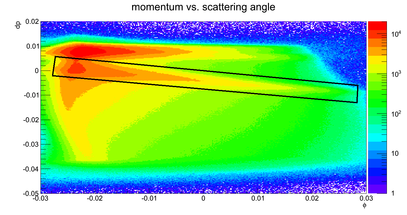
Figure 67: Scattered electron momentum as function of scattering angle. The black rectangle identifies the hydrogen elastic stripe. The data was collected by the left HRS in the 2.2 GeV run.

Fig. 67 shows 2D data of dp vs $\phi$ for the 2.2 GeV runs. The elastic stripes of the different elements are clearly seen, and the hydrogen is well separated from the heavy elements.

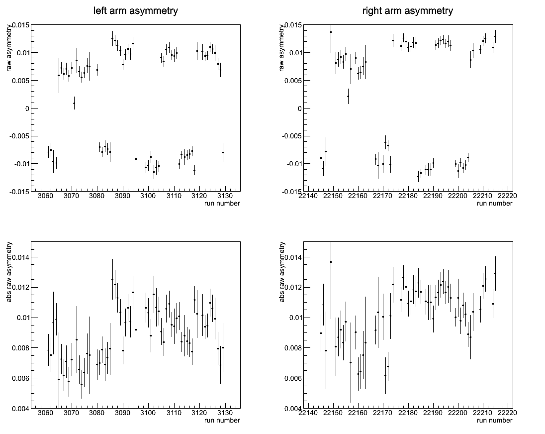
Figure 68: Raw asymmetry as function of run number for the 2.2 GeV data. The asymmetry changes sign due to polarity flipping in the beam and in the target. The bottom plots shows the absolute values of the asymmetries. Note that these are raw asymmetries, without corrections for the polarization of the target and the beam, and dilution.

Raw asymmetries for the 2.2 GeV data shows consistency for both left and right arms (see Fig. 68). The flipping between positive and negative asymmetries is due to changes in target field direction and Half-Wave Plate (HWP) flipping during the experiment. The absolute values of the raw asymmetries does not depend on the target field or the HWP orientation. Based on raw asymmetries for all E08-007-II kinematics, we estimate the statistical uncertainties to be between 1%-2% (depending on bin and bin size).

The dilution factor will be extracted based on experimental data and simulations. Experimental dilution factor values are extracted using He and C runs, as illustrated in Fig. 69.

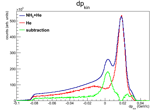
Figure 69: Estimation of the dilution factor using helium data. Subtraction of helium data (red) from the experimental data (blue) reveals what we interpret as hydrogen elastic events (green).

The experimental dilution runs should be corrected for different target thicknesses to be more reliable, and compared to calculations for more precise analysis. The corrections for the asymmetry contribution by the polarized nitrogen has not been studied.

3.11 E08-008 - Deuteron Electrodisintegration

E08-008: Exclusive Study of Deuteron Electrodisintegration near Threshold

B. Norum, A. Kelleher, S. Gilad, D. Higinbotham, spokespersons,

C. Hanretty, Post-Doc,

and

the Hall A Collaboration.

contributed by C. Hanretty.

3.11.1 The E08-008 Experiment

Data for the E08-008 experiment were collected from February 17^th to 23^rd, 2011 in the first experiment to run in the Winter 2011 run period of Jefferson Lab’s Hall A. In this experiment, polarized electrons with 3.358 GeV of energy were delivered to the Hall via the CEBAF accelerator. These electrons were incident on three different target cells (4 cm LH₂, 4 cm LD₂, and 15 cm LD₂), all with unpolarized target materials. Scattered electrons and recoil protons were detected using the Hall’s two High Resolution Spectrometers (HRSs). To reveal the polarization of the recoil proton, a Focal Plane Polarimeter (FPP) was used. This FPP is comprised of an analyzing material placed perpendicular to the proton’s trajectory upstream of a set of two straw chambers. Spin-orbit interactions between the polarized proton and the analyzing material result in asymmetries in the $\phi$-distributions seen in the FPP. Data were collected in this manner for $p(\vec{e},e^{\prime}p)$ and $d(\vec{e},e^{\prime}p)n$ reactions for $x_{B}~{}\epsilon~{}[1,2]$ as seen in Tab. 9.

Table 9: Kinematic settings used in analysis of E08-008 data listed in order of increasing $x_{B}$.

Target Cell	pLHRS	$\theta_{LHRS}$	pRHRS	$\theta_{RHRS}$
4 cm LH2	0.968 GeV/c	57∘	2.95 GeV/c	16∘
4 cm LD2	0.968 GeV/c	57∘	2.95 GeV/c	16∘
15 cm LD2	0.625 GeV/c	68∘	3.14 GeV/c	16∘
15 cm LD2	0.490 GeV/c	68∘	3.14 GeV/c	16∘

3.11.2 Preliminary Analysis

While the physics goal of E08-008 is to measure the ratio $\mu_{p}(G_{Ep}/G_{Mp})$ at low $Q^{2}$ ($x_{B}\rightarrow 2$, where this quantity is sensitive to N-N interactions), data was also taken in the $x_{B}=1$ region for calibration purposes. A preliminary analysis of elastic $p(\vec{e},e^{\prime}p)$ and a brief description of the techniques used are presented here.

Events are first subjected to a series of general kinematic and coincidence cuts to ensure the analysis of properly reconstructed $p(\vec{e},e^{\prime}p)$ reactions. Subsequently, events passing these general cuts are then required to pass cuts specific to the focal plane in the HRS. The first of these cuts is termed the “Conetest” cut which is used to remove false asymmetries based on the detector geometry. Following this cut is a requirement that the angle $\theta_{fpp}~{}\epsilon~{}[5,30)$. The lower limit of this cut removes events that scattered via the Coulomb interaction. Finally a cut is imposed on the secondary scattering vertex which ensures that the analyzed event scattered from the analyzing material.

Events satisfying the above cuts are used to form $\phi$-distributions for each beam helicity setting (+1 or -1). In order to remove any remaining false asymmetries, the asymmetry between the two helicity states is formed via

$$A(\phi)=\left(\frac{N^{+}}{N^{+}_{ave}}\right)-\left(\frac{N^{-}}{N^{-}_{ave}}\right)~{},$$ (32)

where $N^{\pm}$ represents the number of events for a given helicity setting for a bin in $\phi$. These asymmetries are then fit using

$$f^{+}(\phi)-f^{-}(\phi)=y_{0}+A_{y}\left[~{}P^{fpp}_{x}\cos(\phi)-P^{fpp}_{y}\sin(\phi)~{}\right]$$ (33)

where $y_{0}$ is a vertical offset term, $A_{y}$ represents the analyzing power, and the expression

$$f^{\pm}(\phi)=\frac{1}{2\pi}\left(1\pm A_{y}\left[~{}P^{fpp}_{y}\sin(\phi)-P^{fpp}_{x}\cos(\phi)~{}\right]\right)$$ (34)

describes the distribution of events in the FPP as a function of $\phi$. A fit of the helicity asymmetry for $\theta_{fpp}~{}\epsilon~{}[5,30)$ along with the fit results can be seen in Fig. 70.

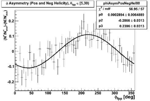
Figure 70: The helicity asymmetry $\left(\frac{N^{+}}{N^{+}_{ave}}-\frac{N^{-}}{N^{-}_{ave}}\right)$ as a function of $\phi$ for $p(\vec{e},e^{\prime}p)$ events in the range of $\theta_{fpp}~{}\epsilon~{}[5,30)$. Also shown is the fit to this asymmetry using Eqn. 33 with the fit results. Here, p0 is the vertical offset ($y_{0}$), p2 = $P^{fpp}_{x}$, and p3 = $P^{fpp}_{y}$. The parameter, p1, corresponds to the analyzing power which is determined using model calculations described in [1, 2] and set as a fixed parameter.

As the ratio $\mu_{p}(G_{Ep}/G_{Mp})$ is calculated from quantities at the target, measurements in the focal plane of the HRS must be transported “backwards” through the spectrometer to the target frame. Two methods are employed to carry out this transport, as described below.

The first of these methods utilizes the ($\phi$) helicity asymmetries seen in the FPP [2]. These asymmetries, instead of being fit to Eq. 33, are fit to an equivalent expression

$$f^{+}(\phi)-f^{-}(\phi)=C\cos(\phi+\delta),$$ (35)

where C is a constant in the fit and

$$\tan(\delta)=\frac{P_{y}^{fpp}}{P_{x}^{fpp}}.$$ (36)

In the dipole approximation, the phase shift $\delta$ as determined from the fit can be used to directly measure the ratio $\mu_{p}(G_{Ep}/G_{Mp})$ via

$$\mu_{p}\frac{G_{Ep}}{G_{Mp}}=\mu_{p}\cdot K\sin(\chi)\left(\frac{P^{fpp}_{y}}{P^{fpp}_{x}}\right),$$ (37)

where the kinematic factor, K, is given by

$$K=\frac{E+E^{\prime}}{m_{p}}\tan^{2}\left(\frac{\theta_{e}}{2}\right),$$ (38)

and $\chi$ represents the precession angle of the proton’s spin through the dipole, given by

$$\chi=\gamma(\mu_{p}-1)\Theta_{bend}.$$ (39)

Seen in Fig. 71 is the fit to the helicity asymmetry (Eq. 32) using Eq. 35 for $p(\vec{e},e^{\prime}p)$ events. Using the results from the fit and Eqns. 36 - 39, $\mu_{p}(G_{Ep}/G_{Mp})=0.873801\pm 0.149866$ for events where $\theta_{fpp}~{}\epsilon~{}[5,30)$.

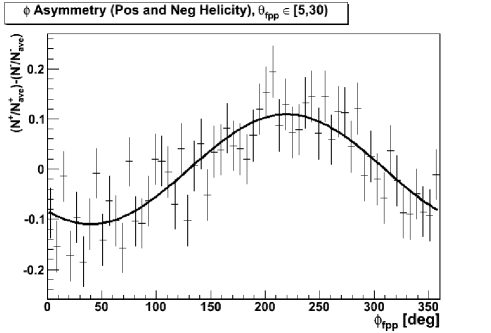
Figure 71: The helicity asymmetry ($\frac{N^{+}}{N^{+}_{ave}}-\frac{N^{-}}{N^{-}_{ave}}$) as a function of $\phi$ for $p(\vec{e},e^{\prime}p)$ events in the range of $\theta_{fpp}~{}\epsilon~{}[5,30)$. Also shown is the fit to this asymmetry using Eqn 35. Here, the phase shift $\delta$ is found to be $-0.6962\pm 0.0838$ rad.

As important quantities such as analyzing power are not constant over the range of $\theta_{fpp}~{}\epsilon~{}[5,30)$, the prudent approach is to bin data in $\theta_{fpp}$ and perform the measurement of $\mu_{p}(G_{Ep}/G_{Mp})$ for each bin. A subsequent fit to these individual measurements can then be performed, allowing for a proper weighting of the data for the entire range of $\theta_{fpp}$. Fig. 72 shows the $\mu_{p}(G_{Ep}/G_{Mp})$ measurements using this method binned in $\theta_{fpp}$ as well as a fit to a horizontal line (in the range of $\theta_{fpp}~{}\epsilon~{}[5,30)$). Here the cumulative result ($\theta_{fpp}~{}\epsilon~{}[5,30)$) is shown as the data point to the far right of the histogram and the horizontal fit result in the stat box. These two quantities, within error, are seen to agree.

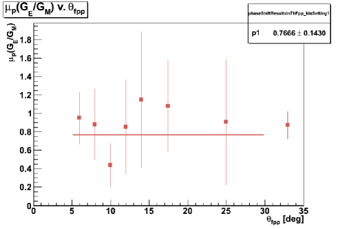
Figure 72: $\mu_{p}(G_{Ep}/G_{Mp})$ measurements using the phase shift method binned in $\theta_{fpp}$. Also shown is a fit to the binned results using a horizontal line (in the range of $\theta_{fpp}~{}\epsilon~{}[5,30)$) and the fit result. Here, the cumulative result is shown as the data point to the far right of the histogram.

The second method used to obtain polarization observables at the target inherits heavily from the Palmetto code used in several Hall A and Hall C analyses. This code, called Sago, uses information from the reconstructed tracks in the FPP and knowledge of the magnetic fields the recoiling proton traverses in the HRS to construct a rotation matrix $\mathbf{S}$. This rotation matrix relates the polarization components in the target ($P_{x}^{tg},P_{z}^{tg}$) to those seen in the FPP ($P_{x}^{fpp},P_{y}^{fpp}$):

$$\mathbf{P^{fpp}}=\mathbf{S\cdot P^{tg}}.$$ (40)

As previously stated, the analyzing power is not constant over the entire range of $\theta_{fpp}$ and events with a higher analyzing power should hold more weight in the analysis. To account for this, Sago uses a weighted sum method when building the rotation matrix ($\mathbf{S}$). The full, explicit form of Eq. 40 can be written as

$$\begin{pmatrix}\Sigma_{i}\lambda_{x,i}\\ \Sigma_{i}\lambda_{y,i}\end{pmatrix}=\begin{pmatrix}\Sigma_{i}\lambda_{x,i}\lambda_{x,i}&\Sigma_{i}\lambda_{z,i}\lambda_{x,i}\\ \Sigma_{i}\lambda_{x,i}\lambda_{z,i}&\Sigma_{i}\lambda_{z,i}\lambda_{z,i}\end{pmatrix}\begin{pmatrix}P_{x}^{tg}\\ P_{z}^{tg}\end{pmatrix}$$ (41)

where $\Sigma_{i}$ represents a summation of the number of events and

$$\lambda_{j}=\eta{h}A_{y}(S_{yj}\sin\phi-S_{xj}\cos\phi)~{}.$$ (42)

Here, $\eta$ denotes the beam helicity, $h$ represents the degree of polarization of the incident electrons, $A_{y}$ is the analyzing power, and $S_{yj}$ (and $S_{xj}$) being elements of the rotation matrix $\mathbf{S}$.

Once these matrices are constructed for the data set, Eq. 41 can be solved for $P_{x}^{tg}$ and $P_{z}^{tg}$ via a matrix inversion. The form factor ratio is then

$$\mu_{p}\frac{G^{p}_{E}}{G^{p}_{M}}=K\frac{P_{y}^{tg}}{P_{z}^{tg}}~{},$$ (43)

where

$$K=-\mu_{p}\frac{E_{e}+E_{e^{\prime}}}{2M_{p}}\tan\frac{\theta_{e}}{2}~{}.$$ (44)

The described method was used to extract the ratio $\mu_{p}(G_{Ep}/G_{Mp})$ for a subset of the e08008 data. For elastic $p(\vec{e},e^{\prime}p)$ events, this ratio was found to be $0.928243\pm 0.155129$. As with the method involving the phase shift, the data (and therefore $\mu_{p}(G_{Ep}/G_{Mp})$) were also binned in $\theta_{fpp}$ and the set of measurements fit with a horizontal line from $\theta_{fpp}~{}\epsilon~{}[5,30)$ (Fig. 73). Here, the fit of the results from Sago binned in $\theta_{fpp}$ can be seen to match the cumulative result within error.

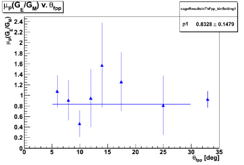
Figure 73: $\mu_{p}(G_{Ep}/G_{Mp})$ measurements using Sago binned in $\theta_{fpp}$. Also shown is a fit to the binned results using a horizontal line (in the range of $\theta_{fpp}~{}\epsilon~{}[5,30)$) and the fit result. Here, the cumulative result is shown as the data point to the far right of the histogram.

Finally, a bin-by-bin and cumulative comparison of the results was carried out as seen in Fig. 74. Shown using the red-brown points are the results from the phase shift method while the Sago results are shown in blue. It can be seen that a comparison of the results, both bin-by-bin and cumulative, shows an agreement between these two methods. Furthermore, a comparison of these (preliminary) results to measurements detailed in [2] show that while the error bars of the Zhan results are much smaller than that of the e08008 (preliminary) results, there is an agreement between measurements.

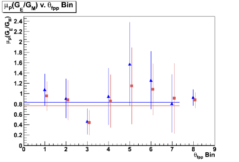
Figure 74: A comparison of $\mu_{p}(G_{Ep}/G_{Mp})$ measurements using the phase shift method and Sago. Here, the red-brown points are the results from the phase shift method while the Sago results are shown in blue. It can be seen that bin-by-bin and cumulatively, there is agreement between the results from the two methods.

3.11.3 Summary

The e08008 experiment conducted during the Winter 2011 run period in Hall A seeks to shed light on the interactions between the proton and the neutron in the deuterium nucleus through a measurement of the ratio $\mu_{p}(G_{Ep}/G_{Mp})$ for $x_{B}~{}\epsilon~{}[1,2]$. Using a beam of polarized electrons and the mechanism of electrodisintegration, data was taken for $p(\vec{e},e^{\prime}p)$ and $d(\vec{e},e^{\prime}p)n$ reactions. Presented here are the results from a preliminary analysis of the elastic $p(\vec{e},e^{\prime}p)$ data using two separate methods which result in a measurement of $\mu_{p}(G_{Ep}/G_{Mp})$ which agree with previous, high-precision results.

3.12 E08-009 - ${}^{4}\mathrm{He}(e,e^{\prime}p)^{3}\mathrm{H}$ at $x_{b}=1.24$

Detailed Study of ${}^{4}\mathrm{He}$ Nuclei through Response Function Separations
at High Momentum Transfers

A. Saha, D. Higinbotham, F. Benmokhtar, S. Gilad, and K. Aniol, spokespersons

and

Students: S. Iqbal (CSULA) and N. McMahon (CNU)

and

the Hall A Collaboration.

contributed by K. Aniol.

3.12.1 Experimental Conditions

The data were taken in collaboration with the SRC(E07-006) measurement during April 13 and April 14, 2011 for 16 hours of running. Our measurements provide the low missing momenta data, 0.153 GeV/c and 0.353 GeV/c which complement the high missing momenta data of the SRC experiment. A 20 cm long cryogenic ${}^{4}\mathrm{He}$ target at 20K and 10 atm provided a thickness of $8\times 10^{22}/\mathrm{cm}^{2}$. The electron beam energy was 4.454 GeV. This is the first measurement of ${}^{4}\mathrm{He}(e,e^{\prime}p)X$ at this value of $x_{b}=1.24$.

3.12.2 Motivation

A theoretical description of ${}^{4}\mathrm{He}(e,e^{\prime}p)X$ is critical for understanding nuclear structure. In particular, one must be able to include many body forces in the theory. The reaction we measured actually includes multiple exit channels, that is, X = ${}^{3}\mathrm{H}$, $n+^{2}\mathrm{H}$ and n+n+p nuclear and nucleonic channels. At the beam energy used here meson production also contributes to X. Our first goal is to compare the data for ${}^{4}\mathrm{He}(e,e^{\prime}p)^{3}\mathrm{H}$ to theoretical calculations provided by the Madrid group [1]. The missing energy spectra also reveal a broad peak attributed [2] to the absorption of the virtual photon on a pair of nucleons.

3.12.3 Preliminary Results

We compare our results to the GEANT simulations. In Fig. 75 we overlay the shapes of the missing energy spectrum for producing the ${}^{3}\mathrm{H}$ ground state, GEANT(blue), with the data for the 0.153 GeV/c kinematic setting. The simulation in this case only includes geometric, energy loss, multiple scattering and radiative effects. The simulation predicts a substantially wider distribution in missing energy.
In Fig. 76 we see the same spectra except now the GEANT simulation includes weighting by the Madrid cross section. There is a dramatic dynamical effect on the width of the predicted missing energy width. In fact, the width of the ground state transition’s missing energy spectrum is very well reproduced by the theory.

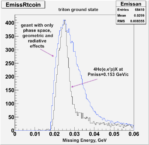
Figure 75: Data(black) compared to GEANT simulation(blue) which does not include weighting by the theoretical cross sections. Peaks are normalized to each other.

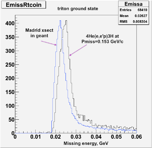
Figure 76: Data(black) compared to GEANT simulation(blue) including weighting by the theoretical cross sections. Peaks are normalized to each other.

The large acceptances of the HRSs allows us to bin the data into smaller missing momentum bites. We show in Figs. 77 and 78 the data for two kinematic settings binned into 0.05 GeV/c bins. Using the GEANT simulation, as described for Fig. 75, we can determine the missing momentum acceptance factor for each bin. These factors enable us to predict a cross section per bin using the theoretical cross sections folded into the GEANT simulation. Preliminary cross sections from the 0.153 GeV/c data are in Tab. 10. Preliminary cross sections from the 0.353 GeV/c data are in Tab. 11. Note that these cross sections do not include subtraction of the background under the triton peak from multi particle break up. An example of the background under the triton peak for the 0.353 GeV/c kinematic setting and a cut on the missing momentum bin from 0.30 to 0.35 GeV/c is shown in Fig. 79.

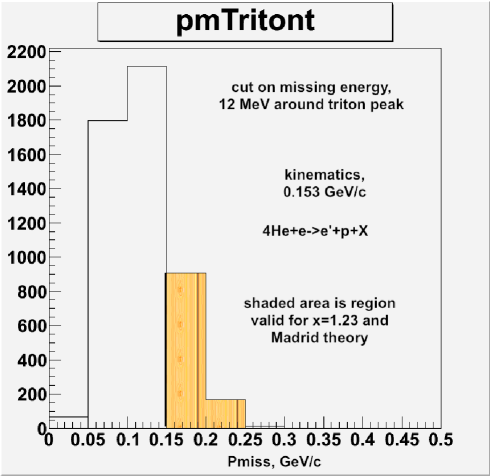
Figure 77: Kinematic setting 0.153 GeV/c. Missing momentum binned in 0.05 GeV/c bins. The shaded area shows which part of the missing momentum is valid for the Madrid theory we have.

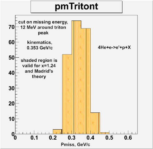
Figure 78: Kinematic setting 0.353 GeV/c. Missing momentum binned in 0.05 GeV/c bins. The Madrid cross sections are valid for all the bins.

Table 10: Preliminary cross sections for the 0.153 GeV/c kinematic settings. Cross sections are in $\mathrm{nb}/\mathrm{MeV}/\mathrm{sR}^{2}$. The Madrid cross sections are available for $P_{miss}$ greater than 0.15 GeV/c for $x_{b}=1.24$.

$P_{miss}$(GeV/c)	Cross Sections $\sigma$	$\delta\sigma$	Madrid $\sigma$
0.0 - 0.05	1.76	0.064	N/A
0.05 - 0.10	0.69	0.009	N/A
0.10 - 0.15	0.191	0.003	N/A
0.15 - 0.20	0.047	0.001	0.0334
0.20 - 0.25	0.0108	0.004	0.0078
0.25 - 0.30	0.0025	0.0003	0.0019
0.30 - 0.35	0.00043	0.0002	0.0012

Table 11: Preliminary cross sections for the 0.353 GeV/c kinematic settings. Cross sections are in $nb/MeV/sR^{2}$. Background from multi particle breakup have not yet been included in the cross section extractions.

$P_{miss}$(GeV/c)	Cross Sections $\sigma$	$\delta\sigma$	Madrid $\sigma$
0.20 -0.25	0.00084	0.0001	0.0098
0.25 - 0.30	0.00064	0.00005	0.0015
0.30 - 0.35	0.00045	0.00003	0.0003
0.45 - 0.40	0.00051	0.0004	0.00019
0.40 - 0.45	0.00040	0.0005	0.00015
0.45 - 0.50	0.00060	0.00015	0.00027

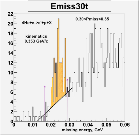
Figure 79: Kinematic setting 0.353 GeV/c. The missing energy spectrum for a cut on the missing momentum bin from 0.30 to 0.35 GeV/c. The background below the highlighted peak still needs to be fitted and removed.

3.13 E08-010 - N $\rightarrow\Delta$

Measurement of the Coulomb quadrupole amplitude at the $\gamma^{*}p\rightarrow\Delta(1232)$
in the low momentum transfer region

S. Gilad, D. W. Higinbotham, A. Sarty and N. F. Sparveris, spokespersons,

Graduate students: D. Anez (St. Mary’s), A. Blomberg (Temple)

and the Hall A Collaboration.

contributed by N.F. Sparveris.

3.13.1 Introduction

Understanding the origin of possible non-spherical components in the nucleon wavefunction has been the subject of an extensive experimental and theoretical effort in recent years [1, 2, 3, 4, 5, 6, 7, 8, 9, 10, 11, 12, 13, 14, 15, 16, 17, 18, 19, 20, 21, 22, 23, 24, 25, 26, 27, 28]. It is the complex quark-gluon and meson cloud dynamics of hadrons that give rise to such amplitudes in their wavefunction which in a classical limit and at large wavelengths will correspond to a ”deformation”. The spectroscopic quadrupole moment provides the most reliable and interpretable measurement of these components; for the proton, the only stable hadron, it vanishes identically because of its spin 1/2 nature. As a result, the presence of resonant quadrupole amplitudes in the $N\rightarrow\Delta$ transition has emerged as the definitive experimental signature of non spherical amplitudes. Spin-parity selection rules in the $\gamma^{*}N\rightarrow\Delta$ transition allow only magnetic dipole (M1) and electric quadrupole (E2) or Coulomb quadrupole (C2) photon absorption multipoles (or the corresponding pion production multipoles $M^{3/2}_{1+},E^{3/2}_{1+}$ and $S^{3/2}_{1+}$ ($L^{3/2}_{1+}$) respectively) to contribute. The ratios CMR $=Re(S^{3/2}_{1+}/M^{3/2}_{1+})$ and EMR $=Re(E^{3/2}_{1+}/M^{3/2}_{1+})$ are routinely used to present the relative magnitude of the amplitudes of interest. Non-vanishing resonant quadrupole amplitudes will signify the presence of non-spherical components in either the proton or in the $\Delta^{+}(1232)$, or more likely at both; moreover, their $Q^{2}$ evolution is expected to provide insight into the mechanism that generate them.

The origin of these components is attributed to a number of different processes depending on the interpretative framework adopted. In the quark model, the nonspherical amplitudes in the nucleon and $\Delta$ are caused by the noncentral, tensor interaction between quarks [29]. However, the effect for the predicted E2 and C2 amplitudes [2] is at least an order of magnitude too small to explain the experimental results, and even the dominant M1 matrix element is $\approx$ 30% low [2]. A likely cause of these dynamical shortcomings is that the quark model does not respect chiral symmetry, whose spontaneous breaking leads to strong emission of virtual pions (Nambu-Goldstone bosons) [28]. These couple to nucleons as $\vec{\sigma}\cdot\vec{p}$, where $\vec{\sigma}$ is the nucleon spin, and $\vec{p}$ is the pion momentum. The coupling is strong in the p-wave and mixes in nonzero angular-momentum components. Based on this, it is physically reasonable to expect that the pionic contributions increase the M1 and dominate the E2 and C2 transition matrix elements in the low-$Q^{2}$ (large distance) domain. This was first indicated by adding pionic effects to quark models [30], subsequently shown in pion cloud model calculations [21, 23], and recently demonstrated in chiral effective field theory calculations [27, 31]. Our current understanding of the nucleon suggests that at low-$Q^{2}$ (large distance) the pionic cloud effect dominates while at high-$Q^{2}$ (short distance) intra-quark forces dominate.

Recent high precision experimental results [3, 4, 5, 6, 7, 8, 9, 10, 11, 12, 13, 15, 16, 17, 18, 19] are in reasonable agreement with predictions of models suggesting the presence of non-spherical amplitudes and in strong disagreement with all nucleon models that assume sphericity for the proton and the $\Delta$. With the existence of these components well established, recent investigations have focused on understanding the various mechanisms that could generate them. Dynamical reaction models with pion cloud effects [21], [22] bridge the constituent quark models gap and are in qualitative agreement with the $Q^{2}$ evolution of the experimental data. These models calculate the resonant channels from dynamical equations; they account for the virtual pion cloud contribution dynamically but have an empirical parameterization of the inner (quark) core contribution which gives them some flexibility in the observables. They find that a large fraction of the quadrupole multipole strength arises due to the pionic cloud with the effect reaching a maximum value in the region $Q^{2}=0.10~{}(\mathrm{GeV}/c)^{2}$ (see Fig. 80). Results from effective field theoretical (chiral) calculations [27, 31], solidly based on QCD, can also successfully account for the magnitude of the effects giving further credence to the dominance of the meson cloud effect in the low $Q^{2}$ region. Recent results from lattice QCD [20] are also of special interest since they are for the first time accurate enough to allow a comparison to experiment. The chirally extrapolated [27] values of CMR and EMR are found to be nonzero and negative in the low $Q^{2}$ region, in qualitative agreement with the experimental results, thus linking the experimental evidence for the nonspherical amplitudes directly to QCD while highlighting the importance of future lattice calculations using lighter quark masses and further refining the chiral extrapolation procedure.

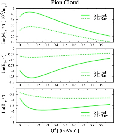
Figure 80: The effect of the pionic cloud to the resonant amplitudes as predicted by the Sato-Lee calculation [21]. Solid line includes the pion cloud contribution while the dashed line neglects the pion cloud effect.

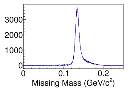
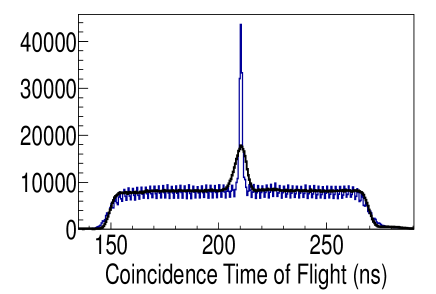
Figure 81: Left panel: The missing mass spectrum for the reconstructed (undetected) pion after the subtraction of accidentals. Right panel: Raw and corrected coincidence Time of Flight spectrum; an excellent timing resolution of 1.6 ns has been achieved after the ToF corrections.

3.13.2 The Experiment

The E08-010 experiment aim to explore the low momentum transfer region at the nucleon - $\Delta(1232)$ transition, where the pionic cloud effects are expected to dominate. The experiment ran in February and March of 2011 and achieved all the quantitative and qualitative goals of the experiment proposal. High precision measurements of the $p(e,e^{\prime}p)\pi^{\circ}$ excitation channel were provided. The two High Resolution Spectrometers were utilized to detect in coincidence electrons and protons respectively while the 6 cm and 15 cm liquid hydrogen targets and an electron beam of $E_{o}=~{}1.15~{}~{}\mathrm{GeV}$ at $75~{}\mu A$ were used throughout the experiment. High precision measurements were conducted in the $Q^{2}=0.04~{}(\mathrm{GeV}/c)^{2}$ to $0.13~{}(\mathrm{GeV}/c)^{2}$ range. The experiment will offer results of unprecedented precision in the low momentum transfer region and will extend the knowledge of the Coulomb quadrupole amplitude lower in momentum transfer. Furthermore these measurements will resolve observed discrepancies between measurements of other labs. Two parallel analysis efforts are currently in progress, by Temple University and St. Mary’s University, in order to ensure the most efficient outcome and to provide important cross checks throughout all the steps of the analysis. At this point the analysis stage involving calibrations has been completed. In Fig. 81 the Missing Mass spectrum (after background subtraction), corresponding to the undetected pion, as well as the corrected time of flight spectrum are presented. An excellent timing resolution of 1.6 ns has been achieved. Currently the effort has moved on to the kinematical phase space analysis, the extraction of the spectrometer cross sections and the extraction of the resonant amplitudes. The projected uncertainties for the CMR are presented in Fig. 82. The new results will allow an in depth exploration of the nucleon dynamics focusing primarily to the role of the pion cloud. A very precise signature of the pion cloud will be provided as well as strong constraints to modern theoretical calculations that will in turn allow for a more complete understanding of the nucleon structure.

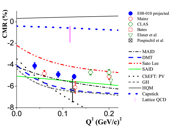
Figure 82: The CMR at the low momentum transfer region. The projected E08-010 uncertainties are presented along with the world data and the theoretical model predictions

3.14 E08-011 - PVDIS

$\vec{e}-^{2}$H Parity Violating Deep Inelastic Scattering (PVDIS) at CEBAF 6 GeV

R. Michaels, P.E. Reimer, X. Zheng, spokespersons,

K. Pan, D. Wang, graduate students,

and

the Hall A Collaboration.

contributed by X. Zheng

The parity violating asymmetry of $\vec{e}-^{2}$H deep inelastic scattering (PVDIS) was measured more than thirty years ago at SLAC [1, 2], and was the first experiment that established the value of the Standard Model weak mixing angle $\sin^{2}\theta_{W}$. The goal of E08-011 is to provide an up-to-date measurement on the $\vec{e}-^{2}$H PVDIS asymmetry. A combination of the quark weak axial charges $2C_{2u}-C_{2d}$ will be extracted and will improve the world knowledge on this value significantly. This experiment also serves as as an exploratory step for the future PVDIS program at the 12 GeV Upgrade.

The PV asymmetry of electron deep inelastic scattering (DIS) off a nuclear target is

$$A_{PV}^{DIS} = -{{G_{F}Q^{2}}\over{4\sqrt{2}\pi\alpha}}\left[2g_{A}^{e}Y_{1}(y)\frac{F_{1}^{\gamma Z}}{F_{1}^{Z}}+{{g_{V}^{e}}}Y_{3}(y)\frac{F_{3}^{\gamma Z}}{F_{1}^{Z}}\right]$$ (45)

$$= -{{G_{F}Q^{2}}\over{4\sqrt{2}\pi\alpha}}\left[a_{1}(x)Y_{1}(y)+a_{3}(x)Y_{3}(y)\right]$$

where $G_{F}$ is the Fermi constant, $\alpha$ is the fine structure constant, $x$ is the Bjorken scaling variable, $y=\nu/E$ is the fractional energy loss of the electron with $E$ the incident electron energy. With $r^{2}=1+{{Q^{2}}\over{\nu^{2}}}$ and $R^{\gamma,\gamma Z}$ the ratio of the longitudinal and transverse virtual photon electromagnetic absorption and the $\gamma-Z^{0}$ interference cross sections, respectively:

$$Y_{1} = \left[\frac{1+R^{\gamma Z}}{1+R^{\gamma}}\right]\frac{1+(1-y)^{2}-y^{2}\left[1-\frac{r^{2}}{1+R^{\gamma Z}}\right]-xy{M\over E}}{1+(1-y)^{2}-y^{2}\left[1-\frac{r^{2}}{1+R^{\gamma}}\right]-xy{M\over E}}$$ (46)

and

$$Y_{3} = \left[\frac{r^{2}}{1+R^{\gamma}}\right]\frac{1+(1-y)^{2}}{1+(1-y)^{2}-y^{2}\left[1-\frac{r^{2}}{1+R^{\gamma}}\right]-xy{M\over E}}~{}.$$ (47)

In the quark parton model,

$$a_{1}(x)=2g_{A}^{e}\frac{F_{1}^{\gamma Z}}{F_{1}^{Z}}=2\frac{\sum{C_{1i}Q_{i}q_{i}^{+}(x)}}{\sum{Q_{i}^{2}q_{i}^{+}(x)}}~{}~{} \mathrm{and} ~{}~{}a_{3}(x)=g_{V}^{e}\frac{F_{3}^{\gamma Z}}{F_{1}^{Z}}=2\frac{\sum{C_{2i}Q_{i}q_{i}^{-}(x)}}{\sum{Q_{i}^{2}q_{i}^{+}(x)}}~{},$$ (48)

where the summation is over the quark flavor $i=u,d,s\cdots$, $Q_{i}$ is the corresponding quark electric charge, $q_{i}^{\pm}(x)$ are defined from the PDF $q_{i}(x)$ and $\bar{q}_{i}(x)$ as $q_{i}^{+}(x)\equiv q_{i}(x)+\bar{q}_{i}(x)$ and $q_{i}^{-}(x)\equiv q_{i,V}(x)=q_{i}(x)-\bar{q}_{i}(x)$. For an isoscalar target such as the deuteron, the functions $a_{1,3}(x)$ simplify to

$$a_{1}(x)=\frac{6\left[2C_{1u}(1+R_{c})-C_{1d}(1+R_{s})\right]}{5+R_{s}+4R_{c}}~{}~{}~{} \mathrm{and} ~{}~{}a_{3}(x)=\frac{6\left(2C_{2u}-C_{2d}\right)R_{v}}{5+R_{s}+4R_{c}}~{}.$$ (49)

Neglecting effects from heavier quark flavors and assuming that $u^{p}=d^{n}$, $d^{p}=u^{n}$ [$u,d^{p(n)}$ are the up and down quark PDF in the proton (neutron)], $s=\bar{s}$, and $c=\bar{c}$, the PDF’s give

$$R_{c}\equiv\frac{2(c+\bar{c})}{u+\bar{u}+d+\bar{d}},~{}~{}R_{s}\equiv\frac{2(s+\bar{s})}{u+\bar{u}+d+\bar{d}}, \mathrm{and} R_{V}\equiv\frac{u-\bar{u}+d-\bar{d}}{u+\bar{u}+d+\bar{d}}.$$ (50)

For E08-011, the central settings of the spectrometer were $Q^{2}=1.121$ and $1.925$ (GeV/$c)^{2}$, while the acceptance-averaged values from data were $Q^{2}=1.085$ and $Q^{2}=1.901$ (GeV/$c)^{2}$. These values are comparable to the SLAC experiment. At $Q^{2}=1.901$ (GeV/$c)^{2}$, the asymmetry was measured to a $\approx 4\%$ (stat.) level. Not including the uncertainty from non-perturbative hadronic effects, the electron and quark neutral weak coupling constant combination, $2C_{2u}-C_{2d}\equiv 2g_{V}^{e}g_{A}^{u}-g_{V}^{e}g_{A}^{d}$, can be extracted from this result. The asymmetry at $Q^{2}=1.085$ (GeV/c)² was measured to a 3% level (stat.), and a simultaneous fit to the asymmetries at both $Q^{2}$ values will set a constraint on the higher twist effect.

The basic running conditions for E08-011 were reported last year. In the past year, our analysis focused on finalizing the systematic uncertainties of the asymmetry measurement. The majority of this analysis has been completed, including corrections due to beam polarization, beam asymmetries, counting deadtime of the DAQ, pion and pair-production background in the electron trigger, beam transverse asymmetries, aluminum endcaps of the target cell, and electromagnetic radiative corrections.

As reported last year, the DAQ deadtime has three contributions: the “path” deadtime caused by summing and discriminating the preshower and shower signals to form preliminary electron and pion triggers; the “veto” deadtime caused by combining the preshower/shower triggers with the HRS T1 trigger and Cherenkov signals; and the “final or” deadtime caused by taking the logical OR of 6 (8) paths to form the final electron and pion triggers for the left (right) HRS. A full scale simulation package was developed to study specifically the timing performance of the DAQ. In the past year, the uncertainty analysis of the deadtime has been completed and a breakdown into these three components are shown in Table 12.

Table 12: Simulated DAQ deadtime loss in percent for all kinematics and for both narrow (n) and wide (w) paths, along with the fractional contributions from group, veto, and OR deadtimes. The fractional deadtime from OR is calculated as one minus those from group and veto, and its uncertainty is estimated from the difference between simulation and the analytical results. The uncertainty of the total deadtime is the uncertainties from group, veto and OR added in quadrature.

HRS, $Q^{2}$	Path	fractional contribution			Total deadtime
(GeV/$c$)2		Group	Veto	OR	loss at 100$\mu$A
Left, $1.085$	n	$(20.6\pm 2.1)\%$	$(51.3\pm 4.5)\%$	$(28.1\pm 4.7)\%$	$(1.45\pm 0.10)\%$
	w	$(29.5\pm 2.4)\%$	$(45.3\pm 4.0)\%$	$(25.3\pm 4.6)\%$	$(1.64\pm 0.11)\%$
Left, $1.901$	n	$(5.42\pm 0.8)\%$	$(81.1\pm 7.1)\%$	$(13.5\pm 7.0)\%$	$(0.50\pm 0.05)\%$
	w	$(8.39\pm 0.4)\%$	$(77.3\pm 6.8)\%$	$(14.3\pm 8.0)\%$	$(0.52\pm 0.06)\%$
Right, $1.901$	n	$(2.9\pm 0.2)\%$	$(80.6\pm 18.5)\%$	$(16.5\pm 12.7)\%$	$(0.89\pm 0.20)\%$
	w	$(4.3\pm 0.4)\%$	$(76.6\pm 17.5)\%$	$(19.1\pm 15.5)\%$	$(0.93\pm 0.22)\%$

The pion contamination in the electron trigger was found to be below $2\times 10^{-3}$, a major accomplishment of the DAQ system specifically built for this experiment, and the effect on the measured asymmetries is negligible.

The blinding factor imposed on the asymmetry analysis was lifted in April 2012. As a result, now we can use “pull” plots to examine the statistical quality of the asymmetry measurement. Here the pull value is defined as

$$p_{i} \equiv (A_{i}-\langle A\rangle)/{\delta A_{i}}~{},~{}$$ (51)

where $A_{i}$ is the asymmetry extracted from the $i$-th beam helicity pair with the HWP states already corrected and $\delta A_{i}=1/\sqrt{N_{i}^{R}+N_{i}^{L}}$ its statistical uncertainty with $N_{i}^{R(L)}$ the event count from the right (left) helicity pulse of the pair, and $\langle A\rangle$ is the asymmetry averaged over all beam pairs. From Fig. 83 one can see that the asymmetry spectrum agrees to five orders of magnitude with the Gaussian distribution, as expected from purely statistical fluctuations.

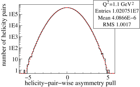
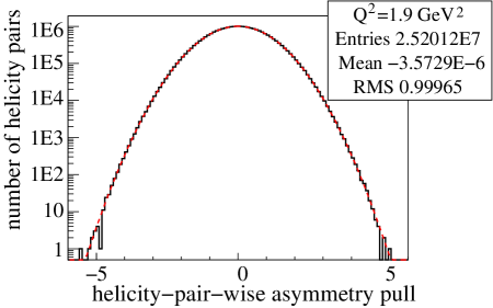
Figure 83: [Pull distribution [Eq.(51)] for the global electron narrow trigger for $Q^{2}=1.1$ (top) and $Q^{2}=1.9$ (GeV/$c$)² (bottom).

Another major focus of past year’s analysis was electromagnetic radiative corrections. These corrections account for the energy loss of both incoming and outgoing electrons due to ionization and bremsstrahlung scattering. Parity violation asymmetries of the nucleon resonances were provided by two models [4, 5] [with [4] for the $\Delta(1232)$ only], and their uncertainties were determined by how well the model agree with our measurement of the resonance PV asymmetries, which were performed with a beam energy of $4.8674$ GeV. Our measured resonance asymmetry for $\Delta(1232)$ is $2-3$ sigma away from both models, but measurements at the $2^{nd}$ and the $3^{rd}$ resonances agreed with the model of Ref. [5] very well. The uncertainty of the radiative corrections was found to be $2\%$ at $Q^{2}=1.085$ and $0.43\%$ at $Q^{2}=1.901$ (GeV/$c$)². Our measurement on the nucleon resonance PV asymmetry will also provide valuable inputs to the box diagram corrections for the Qweak experiment.

In comparing with the asymmetry from the Standard Model, we used the CTEQ/JLab fit, CTEQ6 and CTEQ10 [6, 7], and MRST2008 [8] and MSTW2010 [9] as PDF inputs to Eq.(49). The CTEQ/JLab fit in principle should give the best values since it is tailored to JLab energies, but the fit does not apply to $Q^{2}$ below $1.7$ (GeV/$c$)². By comparing with other PDF fits, the MSTW2010 provides the closest values to the CTEQ/JLab fit, and thus was used to fit the measured asymmetries at both $Q^{2}=1.085$ and $1.901$ (GeV/$c$)². A simultaneous fit of these two measured asymmetries found the higher twist effect to be very small compared to the statistical uncertainty of the measurement.

Currently we are working with theorists to finalize higher-order radiative corrections, in particular the effect from the $\gamma\gamma$ and the $\gamma Z$ box diagrams. We are also extending our analysis scheme to the resonance measurements as well as extraction of the pion asymmetries, and we are aiming to finalize these results within a couple of months. Four draft publications are been worked on: One targeted for NIM which will report on the construction and the performance of the counting DAQ system; one short and one long drafts focusing on the main PVDIS physics results; and one short draft on the resonance asymmetry measurements.

3.15 E08-014 - $x>2$

The $x>2$ Experiment

J. Arrington, D. Day, D. Higinbotham and P. Solvignon, spokespersons,

and

the Hall A Collaboration.

contributed by J. Arrington, P. Solvignon and Zhihong Ye.

3.15.1 Motivations

The shell model has been partially successful in describing many features of nuclei such as the structure and energies of the nuclear excited states. However, about 30-40% of the nucleonic strength predicted by the shell model to be in shells below the Fermi level is not seen in the experimental data [1]. This missing strength is thought to be due to the nucleon-nucleon (NN) interaction at short distances and the fact that the close packing of nucleons in nuclei results in a significant probability of overlapping nucleon wavefunctions. These overlapping nucleons belong to a short range correlated cluster and exhibit high momenta, well above the Fermi momentum in the nucleus [2].

Short-range correlations (SRC) are now well accepted as a key ingredient in the formulation of realistic nuclear wave functions. This means that the experimental characterization of SRC is crucial to the development of accurate nuclear structure calculations. Recent results from JLab experiment E01-015 [3] confirmed the overwhelming dominance of the proton-neutron pairs in two-nucleon SRCs. These two-nucleon knockout experiments are very sensitive to the isospin structure as they are able to measure both pp and pn correlations. However, they have also to deal with potentially large final state interactions which plague coincidence measurements at high missing momentum.

Although inclusive scattering is typically isospin-blind, isospin sensitivity, also called “tensor dominance”, can be identified through a careful choice of complementary targets. Isospin-independent and isospin-dependent models predict 25% differences in the cross-section ratios of the two medium-weight nuclei, ⁴⁸Ca and ⁴⁰Ca. E08-014 complements two-nucleon knockout experiments, for which other physical processes make it difficult to extract a model-independent and precise quantitative measure of the isospin asymmetry. Further insights will be obtained after the JLab 12 GeV upgrade from the use of two light mirror nuclei ³He and ³H [4]; in addition to further enhanced isospin sensitivity in these light nuclei, realistic theoretical calculations can be performed where the nucleon-nucleon potential components and their amplitudes can be separated.

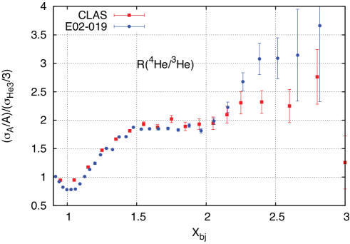
Figure 84: Results from Hall C experiment E02-019 [5]

At $x>2$, the cross-sections from nuclei heavier than deuterium are expected to be dominated by three-nucleon short-range correlations (3N-SRCs). Results from Hall C experiment E02-019 [5] show a discrepancy with the CLAS results [6] in the $x>2$ region, while being in very good agreement the 2N-SRC region (see Fig. 84). E02-019 is at higher $Q^{2}$ than CLAS, and this is consistent with the hint of possible $Q^{2}$ dependence in the CLAS results (see figure 3 of the original proposal [7]). These new data and observations make our measurement decisive in the effort to map precisely the 3N-SRC region and resolve this new issue. E08-014 will also be the first measurement of isospin dependence of 3N-SRC. The amplitude and properties of SRCs have important implications not only for the structure of the neutron stars and their cooling process [8] but also in the search for neutrino oscillation [9].

3.15.2 Analysis status

JLab experiment E08-014 ran in April-May 2011. This experiment aims at mapping the 2N and 3N-SRC scaling behaviors. It should also provide the first test of the SRC isospin dependence in inclusive electron-nucleus scattering by using two Calcium isotopes. This experiment used the standard Hall A high resolution spectrometers configured for electron detection.

The calibrations of all beam diagnostic elements, spectrometer optics and detectors are done and almost all efficiencies have been evaluated. Recently the analysis efforts were directed on the target density study and the observation of a “bump” in the ²H, ³He and ⁴He target length spectra as shown in Fig. 85 for ²H and ³He. It has been determined that this feature was caused by the density fluctuation inside the 20cm long cell. The cooling flow was covering only the upstream half of the cell and therefore the gas/liquid density in this part of the cell was higher than in the downstream half. Also, as expected, this density gradient between the upstream and downstream parts of the cell increases with the beam current. This is mostly an issue for the determination of the target luminosity and the radiative corrections. Data were taken at a range of currents and extrapolated to zero current to determine the overall density change due to beam heating, while the z-dependence of the density as observed from the data is replicated in the simulation to account for the varying density. The cross section are generated versus the variable $x_{bj}$ with each bin being an average over the target length, i.e. $x_{bj}$ does not dependent on the vertex position. However the radiative corrections depend on the location of the reaction. The density distribution along the cell was extracted by fitting the vertex spectra of each cell and then fed into the Monte Carlo simulation to determine the radiative correction factor related to the vertex position.

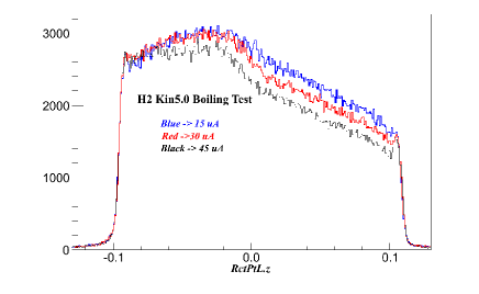
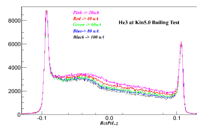
Figure 85: Target spectra along the beam direction for ²H (left plot) and for ³He (right plot).

At present, the main activity is the iteration of the cross section model (Hall C XEM model) in order to fit our kinematical region and then finalize the radiative corrections. Preliminary comparisons of this model to the data are shown in Fig. 86.

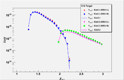
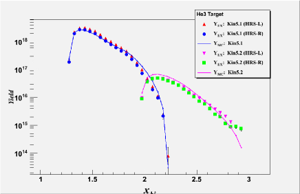
Figure 86: Preliminary carbon (left plot) and ³He (right plot) yields for averaged $Q^{2}$ of 1.8 GeV².

The analysis of E08-014 is in its final stage for the 2N-SRC and 3N-SRC measurements. The isospin study with the data on ⁴⁸Ca and ⁴⁰Ca has been postponed until the cross section model is optimized. Special care needs to be taken for these data because of the non-uniformity of the foils. During E08-014, data were taken to look at the thickness and uniformity of the foils. Even so, the systematic uncertainty of the isospin ratio is anticipated to be higher than previously estimated in the proposal.

3.16 E08-027 - $g_{2}^{p}$

A Measurement of $g_{2}^{p}$ and the Longitudinal-Transverse Spin Polarizability

A. Camsonne, J.P. Chen, D. Crabb, K. Slifer, spokespersons,

and

the Hall A Collaboration.

contributed by R. Zielinski.

3.16.1 Motivation

The inclusive scattering spin structure function (SSF) $g_{2}^{p}$ is largely unmeasured at low and moderate $Q^{2}$ values; the lowest momentum transfer that has been investigated is $1.3$ GeV² by the RSS collaboration [1]. Poor knowledge of $g_{2}^{p}$, along with the other SSFs, in the low $Q^{2}$ region is now a limiting factor in the precision of bound-state QED calculations. The finite size of the nucleon, as characterized by the structure functions has become the leading uncertainty. Furthermore, researchers from PSI [2] have obtained a value for the proton charge radius $\langle R_{p}\rangle$ via measurements of the Lamb shift in muonic hydrogen, which differs significantly from the value from elastic electron proton scattering. The main uncertainties in the PSI results originate from the proton polarizability and from different values of the Zemach radius. These quantities are determined from integrals of the SSF and elastic form factors, which due to kinematic weighting, are dominated by the low $Q^{2}$ region.

The existing data has also revealed a striking discrepancy [3] of $\chi$PT calculations with the longitudinal-transverse polarizability $\delta_{LT}^{n}$. This is surprising since $\delta_{LT}$ was expected to be a good testing ground for the chiral dynamics of QCD [4, 5] due to it’s relative insensitivity to Delta resonance contributions. Measurement of $g_{2}^{p}$ at low $Q^{2}$ will give access to $\delta_{LT}^{p}$ and allow an isospin examination of this ‘$\delta_{LT}$ puzzle’.

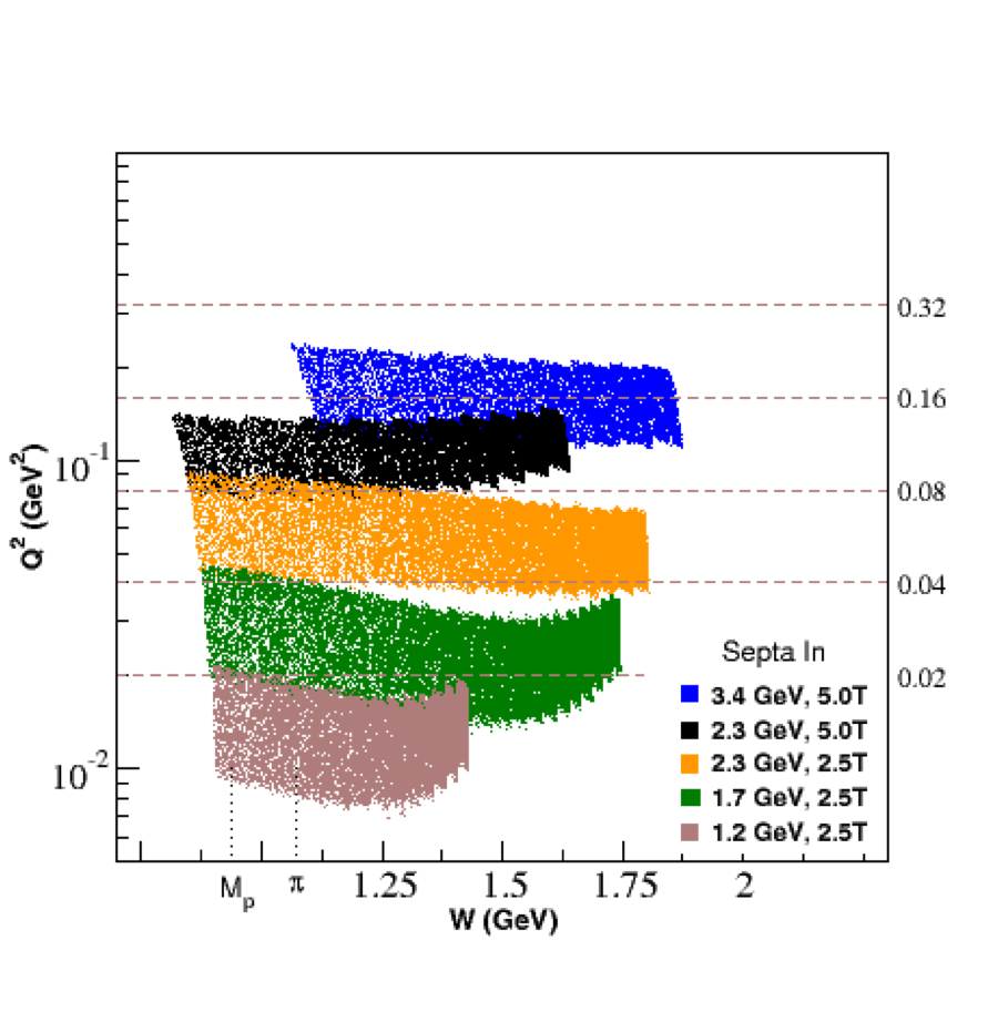
Figure 87: Kinematics covered during experimental run period. The right-hand side vertical axis is the extrapolation to constant $Q^{2}$. As W increases (and momenta decreases) $Q^{2}$ rises due to the target field creating a larger scattering angle.

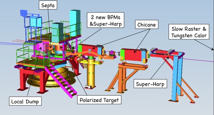
Figure 88: E08-027 installation in Hall A. The third arm detector was located on the left hand side of the bottom target-platform.

3.16.2 The Experiment

The experiment successfully ran March - May 2012 (see Table 13). We performed an inclusive measurement at forward angles of the proton spin-dependent cross sections in order to determine the $g_{2}^{p}$ structure function and the longitudinal-transverse spin polarizability $\delta_{LT}$ in the resonance region for 0.02 $<Q^{2}<$ 0.20 GeV² (See Figure 87). To reach the lowest possible momentum transfer, a pair of room temperature septa magnets were installed to allow detection of scattered electrons at 5.69^∘. During the run period, the right spectrometer (RHRS) septa magnet was damaged twice. After each incident, magnet coils were bypassed, which limited its field strength and momenta range. Dynamical Nuclear Polarization (DNP) was used to polarize the solid ammonia target. The original target’s superconducting magnet coil was damaged during testing, but a similar target was successfully transplanted from Hall B and used during the experiment.

Table 13: Statistics of kinematic settings taken during the run period. Running was split between 2.5 T and 5.0 T target field strength configurations. At lower beam energies (and lower momenta) the 5.0 T target field effectively increased the scattering angle of the detected electrons. This would have limited our low $Q^{2}$ range. To fix this, 2.254 GeV, 1.704 GeV and 1.158 GeV were all run with the target field at half-strength, 2.5 T.

E0(GeV)	Target (T)	Recorded Triggers
2.254	2.5	3.80E+09
1.706	2.5	3.20E+09
1.158	2.5	4.00E+09
2.254	5.0	7.00E+08
3.352	5.0	4.00E+08

The DNP target’s strong magnetic field required the installation of two large dipole magnets upstream of the target to provide chicaning of the beam (see Figure 88). In order to limit depolarization of the polarized ammonia target, the experiment ran low currents ( $\sim$ 50 - 100 nA), which required the installation of two new super-harps and two new M15 antennae style beam position monitors (BPMs) to fully characterize the beam profile. To further minimize depolarization, a slow raster was installed to raster the beam over the entire $\sim$ 2 cm diameter target cup. The lower beam currents also led to the installation of a low current tungsten calorimeter to calibrate the beam current monitors (BCMs).

A new third arm detector was designed for the experiment to give a relative measurement of the combination of beam and target polarization at a 10$\%$ level. The detector counted the elastic recoil protons at large scattering angles in order to measure the elastic proton asymmetry. This asymmetry is related to the beam and target polarization. It was installed on the left-side of the beamline at an angle of approximately 70^∘.

3.16.3 Experimental Progress

A Geant4 based program was developed to simulate the the physics for the high resolution spectrometers (HRS) together with the target and septum fields. The full geometries of the experimental setup have been built in (see Figure 88). This includes the chicane fields for each kinematic setting as well as the two target field configurations and several versions of the septum fields, which are varied in the number of active coils in the right septum. The optics run plan was determined based on the simulation; we will use it to improve optics calibration and determine the spectrometer acceptance.

Currently, spectrometer optics data have been optimized for no target field, chicane set to straight-through running on both the left and right HRS. Straight-though optimization removes the added complexity of the target field and allows for an optics calibration focusing on the septa and HRS magnets. The angle calibration results of the left-HRS straight-through setting are shown in Figure 89. Momentum matrix elements have also been calibrated. Work has now shifted to repeating the same analysis but with a longitudinal target field. The next step is to then determine the optics for the production settings with a transverse target field at both 2.5 T and 5.0 T. The effect of the different right-HRS septa coil packages on the optics for both left and right spectrometer optics is also being analyzed.

Beam position information is also needed for the optics optimization. The straight-through calibration of the BPMs is completed; a new method was created to calculate the beam position from the four-antennae BPMs. The BPM analysis package also includes a transfer function from the BPMs to the target, taking into account the 2.5 T and 5.0 T target fields. The current analysis effort is to create this transfer function. We are also looking into the non-linearity of the slow raster and the issue of increased noise in the BPM signal for low-current running.

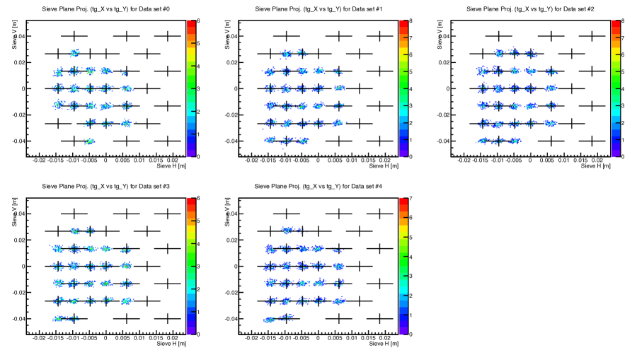
Figure 89: Sieve slit pattern: X vs. Y. Each cross represents the position of the sieve hole used to calibrate the theta and phi angles. The events from each sieve hole have been aligned well as a sieve pattern is clearly visible. Five panels represent different delta scan runs, which together represent the focal plane momentum coverage, -3.5$\%$, -2$\%$, 0, 2$\%$, 3.5$\%$, respectively.

Spectrometer detector efficiencies are needed as a correction to the measured cross section. A first round calibration of the HRS detectors is now completed. This includes particle identification (PID) calibrations on the gas  Čerenkov and lead glass on both spectrometer arms. Detector and cut efficiency analysis on the PID detectors is currently underway. The S1 and S2m trigger scintillator efficiency is also finished for both arms. The results for the left-HRS are shown in Figure 90. The trigger efficiency for all good production runs is above 99$\%$.

An electron asymmetry measurement is needed along with the absolute cross-section to extract $\delta_{LT}^{p}$. For the asymmetry measurement, beam helicity information is needed. The experiment used the helicity scheme set by Qweak, which was also used in the DVCS experiment. The g${}_{2}^{p}$ helicity decoder package is a combination of the DVCS and normal Hall A decoders. The package has already been tested during the production running and worked well with very preliminary asymmetries calculated during the production run period.

Measurements of the target polarization are also needed to determine the asymmetries. The calibration constants, used to convert the NMR signal into a polarization, for all target materials and settings have been calculated. They can now be applied to the polarization signals on a run by run basis to obtain averaged target polarizations with relative uncertainties in the 1-4$\%$ range. Still to be done is a quality check of the target NMR signal throughout the experiment, along with some polarization signal fit adjustments to reduce uncertainties.

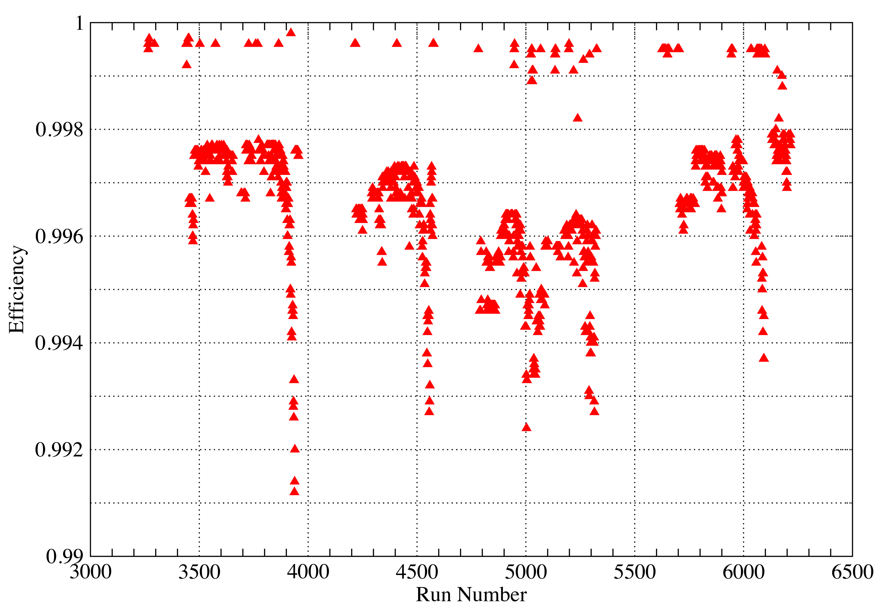
Figure 90: Left-HRS trigger efficiency results for all production runs.

Following the completion of the target analysis, base optics and BPM calibrations, and first round detector calibrations, the experiment is beginning to move into first-pass farm production. Optics will continue with the effort moving to optimization of the production settings and the BPM calibrations for the same settings. The GEANT simulation will also be used to begin work on determining the experimental acceptance needed for a cross section measurement. The detector efficiencies will be finalized, and we will start the asymmetry-dilution analysis, which determines what percentage of the electrons detected by the HRS were not scattered off of a proton from the ammonia target.

3.17 E12-06-122 - $A_{1}^{n}$

Measurement of the Neutron Asymmetry A1n in the Valence Quark Region Using 8.8 and 6.6 GeV Beam Energies and the BigBite Spectrometer in Hall A

contributed by J. Annand, T. Averett, G.D. Cates, N. Liyanage, G. Rosner, B. Wojtsekhowski, and X. Zheng.

The PAC36 report said the following about the Hall A A1n experiment:
“These experiments exploit the Hall A and C spectrometers to measure the down quark polarization $\Delta$d(x) at the highest possible value of x and level of statistical precision (i.e., beyond that accessible at CLAS). Their use of a ³He target also provides an important systematic check on possible nuclear effects in the extraction of $\Delta$d. PAC30 approved the Hall A experiment, but conditionally approved the Hall C experiment as it was not convinced that Hall A could not be used for the entire program. The case made at PAC30 was that the Hall A Bigbite spectrometer with an added Cherenkov detector would not provide sufficient pion rejection to reach the highest x and Q² points of the Hall C proposal. As the Hall A experiment would likely run near the start of 12 GeV data taking, it seemed sensible to simply wait and see how Bigbite performed before making a final decision on the need for further data from Hall C.

The updated proposals reviewed by PAC36 included numerous changes that made the two experiments much more similar. Perhaps most importantly, the beam time request for the Hall C was greatly reduced: from 79 to 36 days, which is commensurate with the 23 days requested at Hall A. Both experiments propose to take two stripes in (x,Q²) that give each a Q² lever arm up to similar values of x (0.6 for Hall A and 0.55 for Hall C). Both have hardware issues. At Hall C, the dramatic reduction in beam time was accomplished by proposing a major upgrade of the target that would permit it to withstand a 60 $\mu$A beam current. Significant R&D will be required to accomplish this technical goal. At Hall A, a more modest target upgrade was invoked (for 30 $\mu$A maximum beam current), but the new Cherenkov detector proposed for Bigbite was revealed to be a RICH with a finely segmented array of over 1,000 phototubes. The PAC was pleased to see that manpower (the Averett group) was clearly identified for this task, but even with the recycling of parts from the decommissioned HERMES RICH, this is an ambitious undertaking.

With the Hall A and Hall C A1n proposals now on a near-equal footing in terms of beam time and experimental complexity, the PAC concluded that they should have equal approval status. The difference in letter grade arose from the experiments’ kinematic reach. The Hall C experiment has two small but distinct advantages in this area, thanks to its use of the full 11 GeV beam energy. First, the top x value of 0.77 is the highest of all the g1 experiments. Though this value is only slightly above the 0.70 accessible at Hall A, the PAC found Wally Melnitchouk’s arguments persuasive: the non-linear behavior of higher-twist, target mass, and other corrections in the quest for the x$\rightarrow$1 limit of the PDFs makes a strong case for pursuing even slight improvements in x range. Second, the Hall C experiment has the broader Q² range (2-8 GeV² as compared to 2-5 GeV² at Hall A), which is also important for constraining higher twist contributions.”

Since the approval of the proposal, the collaboration has put all efforts into development of the instrumentation which is briefly outlined below.

3.17.1 Configuration of the BigBite spectrometer

The detector configuration was outlined in the presentation to PAC36. It includes the front tracker, the Gas Cherenkov counter, the rear chamber, the two-layer shower calorimeter, and the timing hodoscope. Following the PAC advice, we have reconsidered the source of the PMTs for the Gas Cherenkov counter and decided to use the 29 mm PMTs from the DIRC detector of BABAR instead of the HERMES RICH PMT array. The detector configuration was presented to the DOE review in October 2011, which reviewed the SBS projects, as well as “the dependencies” such as the Bigbite, which will be used as an electron arm in two form factor experiments and in the SBS SIDIS experiment. These detectors are under construction by the collaboration. The INFN collaborators are in charge of the front tracker. UVa is providing the larger rear chamber. Glasgow University is leading construction of the timing hodoscope. W&M is leading development of the Gas Cherenkov counter. Most of the funding required for such an upgrade of the Bigbite detector is being provided by users. However, about $70k is requested from Hall A for the construction of a vessel of the Gas Cherenkov counter and its front-end electronics. The following sections present the status and configuration of those detectors.

3.17.1.1 Gas Cherenkov

1. The focus of the experiment is to measure $A_{1}^{n}$ with a statistical precision on the level of 0.003 and similar systematics. Thus we will require the Cherenkov detector to have $\eta_{\pi}^{GC}\leq 0.1$ while assuming modest performance of the lead-glass system: $\eta_{\pi}^{LG}=0.1$, where $\eta_{\pi}^{GC}$ and $\eta_{\pi}^{LG}$ are the pion detection efficiencies for gas Cherenkov and lead-glass respectively.

2. The detector must fit within a 90 cm keep-out zone between the GEM chambers in the new BB detector frame. This requires the maximum length of GRINCH is $\leq$ 85 cm.

3. In the $A_{1}^{n}$ experiment, the Bigbite spectrometer is set at a scattering angle of $30^{\circ}$. The target length will be 60 cm, compared with 40 cm used previously which brings the total material in the beam from 0.31 g/cm² to 0.36 g/cm². The beam current will be increased from $12.5\,\mu$A to $40\,\mu$A. These factors will increase the total luminosity by a factor of 4, assuming no other changes to the material in the beamline. Assuming the worst case scenario, with no improvement to the beamline, the background rates are also expected to increase by a factor of 4. To separate the signals from the large background, few improvements have to be applied.

   1. The Cherenkov ring will be detected by an array of 29mm diameter Electron Tubes 9125B PMTs with 25mm active diameter. The surface area of these PMTs compared with those used in $d_{2}^{n}$ (5”) is 0.052. In addition, the face of the PMTs is made from glass that is 3x thinner. A (8)9x30 array of tubes, where 8 for even rows and 9 for odd rows will be instrumented with custom NINO-based front end electronics that include an amplifier, discriminator and pulse height sensitivity to provide a crude measurement of the pulse height. The NINO boards will be connected to FASTBUS multi-hit TDCs. We may also have FASTBUS ADCs that could be used for low rate running and calibration.

   2. The primary information from the detector will be timing-based. Spatially localized clusters of PMTs that detect a signal within a 10 ns timing window will be identified in the offline analysis. Based on simulation, the average number of photoelectrons produced per tube is expected to be around 2.5, and on average 9 PMTs are expected to “fire” ($\geq 1$ p.e.) for an electron event. The discriminator thresholds will be set to approximately 20-30% of the single ph.e. peak to provide good detection efficiency for single p.e. hits. Offline analysis will be even less sensitive to background as the timing cut is reduced to $<10$ ns.

   3. The PMT array will be located on the large angle side of Bigbite where the rates are 10x smaller as demonstrated in the Hall A technical note for the Bigbite Cherenkov Detector[5].

   4. The heavy gas radiator $\mathrm{C}_{4}\mathrm{F}_{8}\mathrm{O}$ with index $n=1.00135$ at 1 atm and as long active length of gas as possible will be used to generate enough photons to identify the electrons. And the index gives a pion threshold of 2.7 GeV/c.

4. Because of the open geometry of the Bigbite magnet, there is a significant magnetic field (of 15 Gauss) at the PMT location. This requires the shielding should be added in the final design.

5. Experimental studies [6] have demonstrated that neutron induced $\alpha$ particles have a very short path in the glass and a negligible probability of inducing a signal in the PMT. The probability was found of $3\times 10^{-4}$ for the borosilicate window R7525-HA and $3\times 10^{-6}$ for the quartz window R7600U-200-M4 PMTs, respectively. Again note that the thickness of the glass window of the 29 mm PMTs is 3x less than the 5” tubes. The contribution of neutrons to the background by conversion in the PMT glass is expected to be very small relative to the electromagnetic background discussed next.

   The Monte Carlo simulations [7] have shown that a significant background of low-energy electrons is present due to production from material near the beam line and in the target scattering chamber which was not under vacuum. Bench tests [8] have shown that $\sim 1$ MeV electrons from a ¹⁰⁶Ru source will produce Cherenkov radiation in the PMT glass which produces a single-photoelectron hit 30% of the time. Reasonable agreement between MC and the measured rates in $d_{2}^{n}$ was achieved. Using this information, we can estimate the background contribution from this process, which again will be reduced by a factor of 3 due to smaller glass window thickness. Another source of background is photons that are produced in Bigbite or via line of sight to the target or beam line.

To satisfy these requirements, simulation and optimization of the proposed design has been completed using Geant4 to optimize the geometry of the vessel and the detector array. The optimization was focused on producing the largest possible electron efficiency and pion efficiency. This translates to generating the largest number of photo-electrons per tube per event with the smallest possible Cherenkov ring diameter.

In the Geant4 simulation, the detector vessel with an average active path length of 66 cm are installed with entrance (40cm(W)x150cm(H)x0.01cm(T)) and exit windows (50cm(W)x200cm(H)x0.01cm(T)) shown in Figure 91. It will be attached to the gas vessel such that 4 cylindrical mirrors with radius of curvature 1.3 meters can be used to transport all Cherenkov light onto the array. As mentioned previously, the PMTs with glass on the front surface, light-catchers and 61 iron/mu-metal magnetic shielding bars will be arranged in a tall, narrow array located on the large angle side of the BB spectrometer. The distance from mirror center to the front surface of PMT is 65 cm. Angle between beam and PMT array is $55^{\circ}$. The detector will be filled with 1 atm (absolute) of the “heavy gas” C₄F₈O. The above selected geometry will provide an average of 2.5 photo-electrons per tube, and an average of 9 tubes will fire for an event.

Figure 91: GRINCH Tank.

• Four mirrors are stacked as shown in Figure 91. The size of middle two mirrors (red and blue) is 70cm(W)x60cm(H), for the top and bottom ones (gray and green) is 70cm(W)x40cm(H). Mirrors could be made using a technique that has been proven in the HRS Cherenkov detectors [9] and in the CLAS6 spectrometer. A thin Lexan sheet, which is a polycarbonate material because it has less trouble with stress at the surface than acrylic, will be formed using pressure and heat to achieve the desired curvature. This sheet will be coated with reflective aluminum and the back will be glued to honeycomb or low-density foam, followed by an outer shell. Because this detector is not based on the concept of focusing a given ring onto a single PMT, it is much less sensitive to mirror geometry. Cylindrical mirrors instead of the usual spherical mirrors will be used, making fabrication easier and potentially cheaper. Cylindrical mirrors are sufficient for transporting the light to a PMT array.

• Recently, several thousand PMTs were obtained by Hall A from the decommissioned BaBar DIRC detector [10], and some PMT bases and HV cables were included. There they were used in a ring-imaging Cherenkov detector that transported light from quartz crystal radiators to the using water. The tubes were removed after 10 years of service, and the faces of the tubes showed signs of surface damage due to immersion in ultra-pure water. The quantum efficiency of the tubes was found to have decreased by approximately 20-25% [11]. A thin disk of fused silica was glued onto the window at Jefferson Lab and 70 of these tubes were tested for dark noise/current, gain and relative quantum efficiency [12]. Data from before and after adding the glass disks were compared. The average increase in quantum efficiency was  10% after adding the glass disks. The PMTs will be mounted in a hexagonal close packed configuration with a spacing of $31$ mm, which means the sensitive area of the PMTs will cover $\sim 60\%$ of the area of the array (see Figure 92). Each tube will be outfitted with a reflective cone attached to the perimeter of the photocathode as the yellow component shown in Figure 92(a). The cone will be constructed from thermoplastic with a reflective coating and will be used to collect light that is not incident on the active area of a given tube. Based on simulation, we expect a 20% increase in the number of detected photons.

  

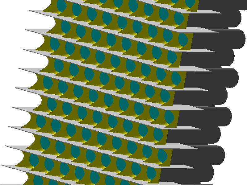
  (a) Array 3D view.

  

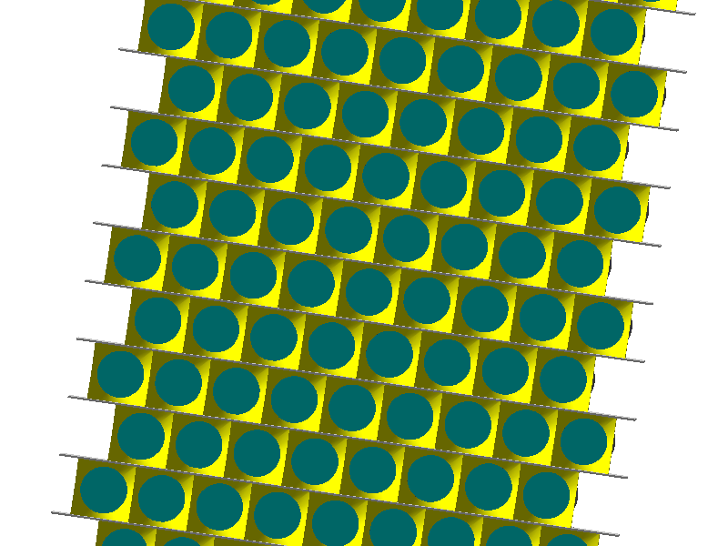
  (b) Array Front view.

  

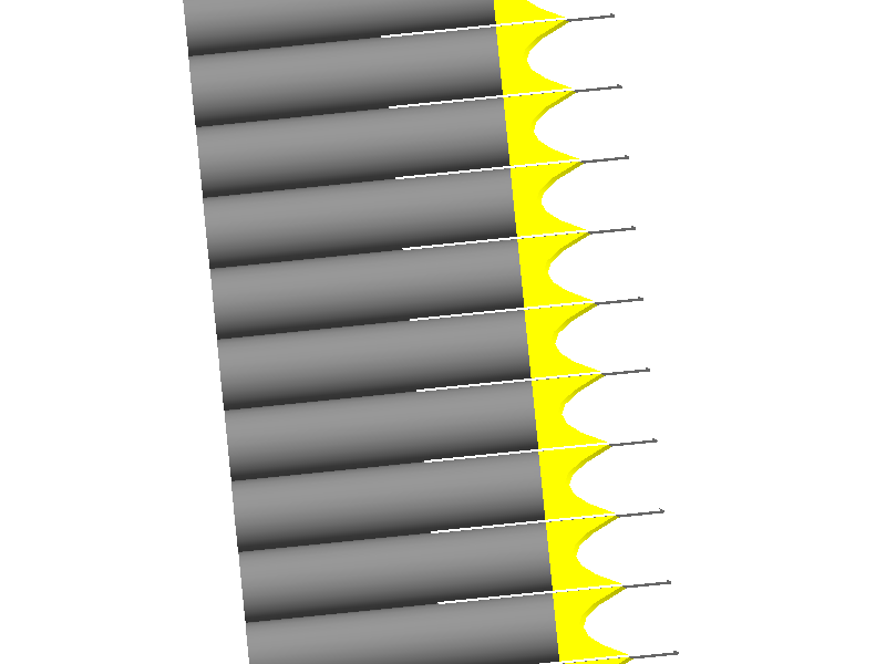
  (c) Array Side view.

  

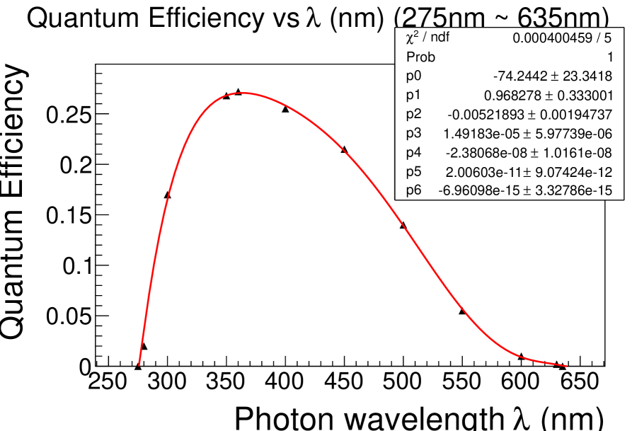
  (d) PMT quantum efficiency.

  Figure 92: PMT array. White is shielding bars (29.9cm(W)x10cm(H)x0.1cm(T)),half of height is below PMT surface. Cyan is glass layer with 3mm thickness on PMT. Yellow is light-catcher. Grey is insensitive area of PMT and blue is sensitive area (25mm diameter).

• The array will be surrounded with a rectangular steel (1010) box with five sides, the sixth side being open for the faces of the PMTs, which are located approximately 5 cm down inside the box. The detector and shielding geometry is being studied using TOSCA. The properties of the BigBite field at the PMT array are well understood from TOSCA simulation and measurements. PMT dynodes will be oriented horizontally to minimize the effect of the residual magnetic field.

In the MC simulation, the electron detection efficiency $\eta_{e}$ is defined as the probability that an incident electron will be detected as a good electron event. The pion detection efficiency $\eta_{\pi}$ is defined as the probability that an incident pion will be detected as a good electron event.

At pion momenta below the Cherenkov threshold, $\eta_{\pi}$ is limited by the delta electron knockout process in the gas, which has probability of 2%. The total number of p.e.’s in that process has a wide distribution due to variation of the origin of the delta-electron along the pion track through the gas.

Figure 93(b) shows the pion detection efficiency $\eta_{\pi}$ for the different amplitude thresholds, averaged over momentum 1.6-3.3 GeV/c. The $\pi/e$ ratio increases as momentum decreases. We will require $\eta_{\pi}\leq 0.1$. Using Figure 93(b) with 1 atm of gas, we require $\geq 11$ photoelectrons. Using this cut, Figure 93(a) gives electron efficiencies of $\eta_{e}\sim 0.98$ (est.) for 1  atm.

The electronics for the GRINCH may provide some pulse-height information which would allow us to make a crude measurement and cut on the number of photoelectrons, but the detector is designed to work using timing clusters. Therefore, if we are to make a cut at 9 p.e.’s, what we really need is a cut on the number of PMTs fired that will be efficient for requiring 9 or more p.e.’s per event.

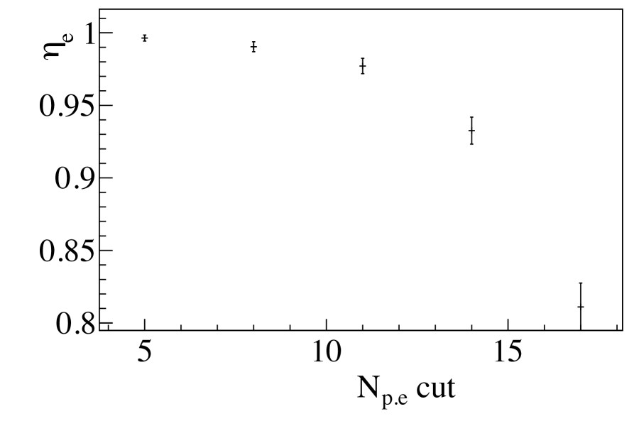
(a) $\eta_{e}$ for different $N_{p.e}$ cut.

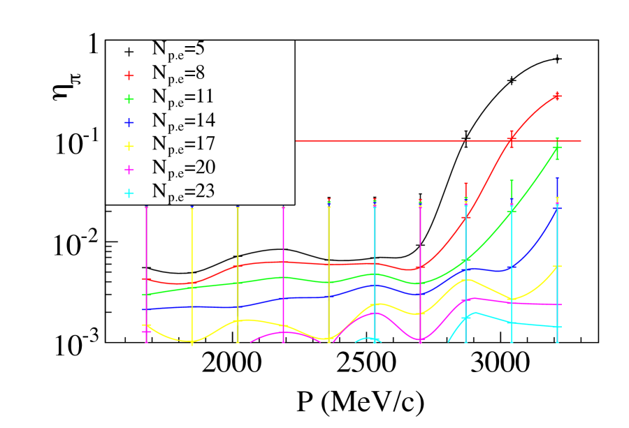
(b) $\eta_{\pi}$ for $P$ for different $N_{p.e}$ cut.

Figure 93: Efficiency

3.17.1.2 Timing Hodoscope

The A1n experiment, in common with many new JLab experiments, plans to run the BigBite spectrometer at higher luminosity than previously achieved in Hall A. To accomplish this, the detector stack of BigBite is being upgraded. Part of this upgrade involves an increase in the segmentation of the plastic scintillator hodoscope, used to determine the time of an electron hit precisely. The new hodoscope will consist of 90 elements of EJ200 plastic (Fig.94), each of size $25\times 25\times 600$ mm and each read out at either end of the bar via 24 mm diameter lucite light guides. The PMT is clamped in position at the end of the light guide by a housing, which excludes both stray light and any He in the Hall A atmosphere. Since the cross section dimensions of a bar are less than the diameter of the PMT housing, each alternate element has curved light guides to allow the bars to be packed closely. The PMTs are type ELT9125 units, which have been obtained from the BaBar spectrometer. They were originally used on a DIRC system, and when coupled to a scintillator, the output pulse was found to saturate. This has been cured by a redesign of the PMT voltage divider base.

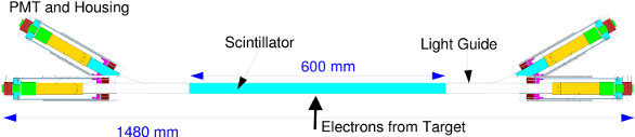
Figure 94: Top view of the BigBite timing hodoscope elements.

The hodoscope is under construction in Glasgow and one bar has been tested using cosmic rays. The interaction position of the cosmic rays was localized using 2 trigger plastic scintillators of size $40\times 40\times 10$ mm placed above and below the bar. Fig.95 shows the variation in the pulse form from a single PMT (1) attached to the hodoscope bar, as the trigger counter is moved along the length of the bar. The rise time from the PMT is $\sim 4$ ns, which is relatively slow for a 28 mm diameter linear focused PMT, and the total pulse length from a hodoscope bar is $\sim 25$ ns.

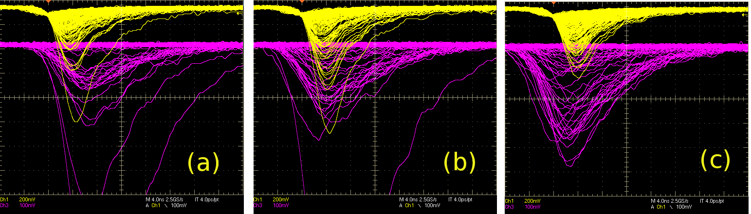
Figure 95: Pulses from PMT.1 of the hodoscope bar under test (magenta) and the upper trigger counter (yellow). a) Trigger the far end of the hodoscope bar. b) Trigger at the middle of the hodoscope bar. c) Trigger at near end of the hodoscope bar.

Both trigger and hodoscope signals were fed into a NINO card (Sec. 3.17.1.3) and in addition the trigger signals were split and fed to 2, type 934 Ortec Constant Fraction Discriminators (CFD). The latter provided reference times and also a physical trigger signal for the DAQ system. Pulse amplitudes from the NINO card were recorded by a CAEN V792 QDC and times recorded by a V1190A multi-hit TDC, which accepts LVDS signals and has 100 ps resolution. The TDC was programed to record both the leading and trailing edges of the logic pulses, so that time over threshold could be measured. This is correlated to the pulse amplitude, and is intended for time walk correction. The CFD NIM-logic outputs were converted to LVDS and also input to the V1190A.

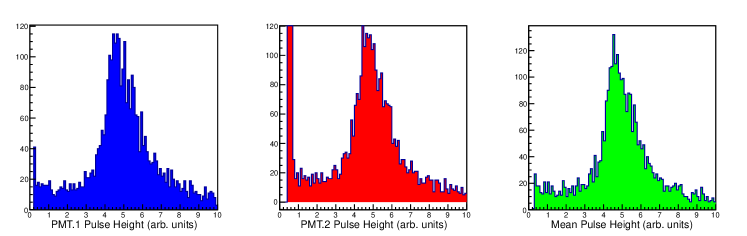
Figure 96: Pulse amplitude spectra from the hodoscope bar (blue: PMT.1, red: PMT.2, green: geometric mean pulse height of PMT 1 and 2).

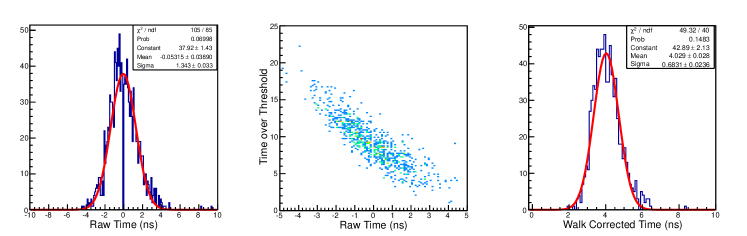
Figure 97: TDC spectra for PMT.2. The left panel shows the uncorrected coincidence time distribution. The middle panel shows the same distribution plotted against the pulse time over threshold (walk effects). The right panel shows the coincidence time distribution after correction for walk.

Data were recorded with the trigger scintillators placed at various points along a hodoscope bar. Fig.96 shows pulse height spectra from the two PMTs attached to the bar and the geometric mean pulse height, given by $Q_{mean}=\sqrt{Q_{1}Q_{2}}$. The TDC spectrum from PMT.2 is shown in Fig.97 (left). When plotted against the time over threshold (middle) the effect of time walk is evident. The walk effect was corrected, assuming a linear dependence of walk on time-over-threshold, producing the distribution on the right panel. The hit time in a hodoscope bar is obtained from the mean time of the 2 PMTs $T_{mean}=(T_{1}+T_{2})/2$ and the hit position along the bar from the time difference $T_{diff}=T_{1}-T_{2}$. Typical distributions are displayed in Fig.98. The mean-time resolution of the hodoscope bar is $\sim 0.4$ ns while the time-difference resolution is $\sim 0.7$ ns. By comparison the coincidence time resolution of the top/bottom trigger detectors using a CFD is $\sim 0.4$ ns.

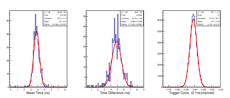
Figure 98: Coincidence time distributions. Left: mean time $T_{mean}$, center: time difference $T_{diff}$, right: top-bottom trigger coincidence.

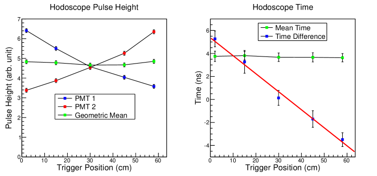
Figure 99: Variation of pulse height (left) and hit time (right) as the trigger position is varied. The pulse height is obtained from the minimum-ionizing peak position. The error bars on the time plot are the widths obtained from Gaussian fits. The red line is a linear fit to the time-difference dependence.

The variation in pulse height and timing distributions for different positions of the trigger counters is shown in Fig.99. While the pulse height from individual PMTs varies significantly over the length of the bar, the geometric mean is almost position independent. Similarly the mean time is position independent while the time difference dependence on position is approximately linear. A linear fit to the time difference dependence produces a slope of -0.16 ns/cm which translates to a position resolution along the bar of $\sim 4.5$ cm.

3.17.1.3 Front-end NINO card

The GRINCH gas Cerenkov and Timing Hodoscope components of the BigBite detector stack will employ the best part of 1000 photomultipliers (PMT) for readout and will use PMTs, originally from the DIRC system of the BaBar spectrometer. The electronics will be mounted close to the PMTs to avoid long runs of coaxial cable, and must therefore be compact and economical on power consumption. A low cost implementation, based on the NINO ASIC [3] from CERN, has been designed. NINO was designed originally for the Multigap, Resistive Plate Chambers (MRPC) which form the time of flight systems at the ALICE experiment at LHC. It expects to receive a differential input signal and thus, for the present PMT application, some additional circuitry is required. A diagram of the NINO circuit for BigBite and general Hall-A use is given in Fig. 100.

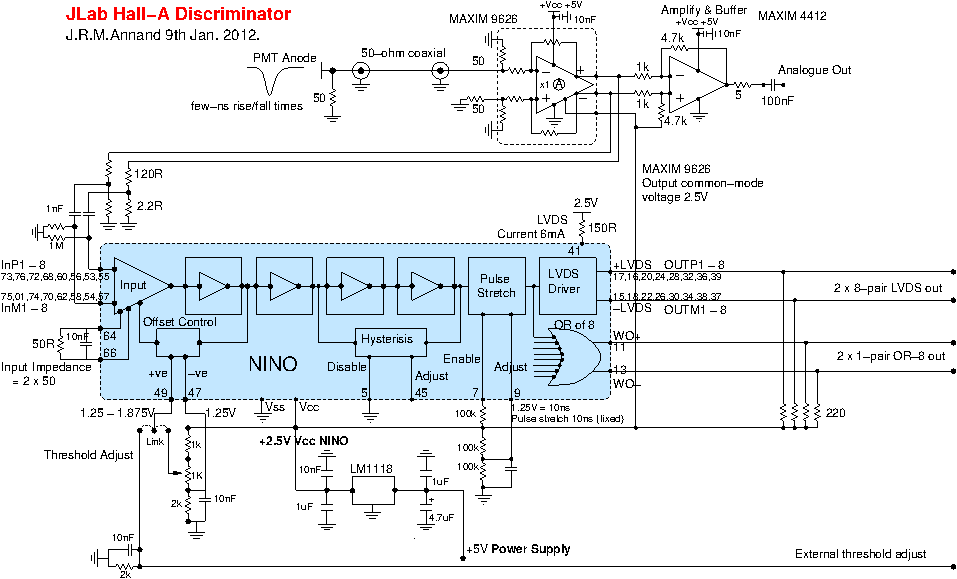
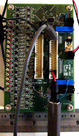
Figure 100: Left: circuit diagram of the NINO based amplifier/discriminator card. Right: photograph of the prototype NINO card under test at Glasgow.

Each NINO ASIC has 8 discriminator channels and the Hall-A card (Fig. 100 right panel) will mount 2 of these, giving 16 channels in total. On each channel the signal from the PMT anode is input, via coaxial cable, to a fast, fully-differential amplifier (MAXIM 9626). The differential output from this unity-gain amplifier is then attenuated and fed to the NINO input. The MAXIM 9626 output also feeds to a buffer stage (MAXIM 4412), providing an output for pulse amplitude measurement.

The 16 NINO logic outputs conform to LVDS standard and in addition 2 OR-of-8 LVDS outputs are provided. The LVDS outputs operate in time-over-threshold mode, where the width of the logic pulse is the duration that the input analogue pulse exceeds the discriminator threshold plus 10 ns. Each NINO ASIC has a common threshold circuit for the 8 channels, and the threshold level may be adjusted via an on-board potentiometer or external voltage level. A voltage difference of 650 mV applied to the threshold circuit (Fig. 100) produces a threshold voltage of 180 mV on the input signal, equivalent to a charge of $\sim 45$ pC for the hodoscope signal. The relation of voltage difference on the threshold circuit to PMT output voltage is given in Fig. 101. The overall range may be shifted by changing or removing the attenuation factor for pulses input into the NINO chip.

The card is powered by a single +5 V supply and draws 1.76 A. The +2.5 V necessary for the NINO chips is derived from +5 V using an on-board voltage regulator.

Tests of the performance of the discriminator card in conjunction with elements of the timing hodoscope is described in Sec.3.17.1.2.

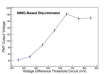
Figure 101: Relation of voltage difference on the threshold circuit with PMT output voltage.

3.17.2 High Luminosity polarized ³He target

The most important requirement for the polarized ³He target for the Hall A $A_{1}^{n}$ experiment is the ability to maintain high polarization despite being run at high luminosity. Indeed, this requirement is shared by most of the other 12 GeV-era experiments that will use polarized ³He targets. Another key feature is cost. Here, it is important to consider both the cost of the target that is being built specifically for $A_{1}^{n}$, as well as the polarized-target costs that will be incurred as the 12 GeV program progresses.

The $A_{1}^{n}$ polarized ³He target will be based on alkali-hybrid spin-exchange optical pumping [13], a variant of spin-exchange optical pumping that has resulted in significant improvements in target performance [14]. While the design of the $A_{1}^{n}$ polarized target is still in progress, one feature that is settled is that it will have “convection-based gas flow”. The polarized ³He targets are sealed glass cells, and they have historically included two chambers, a pumping chamber in which the ³He is polarized, and a target chamber through which the electron beam passes. With convection-based gas flow the transfer of gas between the two chambers, proposed back in 2002 by B. Wojtsekhowski [15], is much more rapid than was the case in earlier designs. The convection-based cells, the basic geometry of which is illustrated in Fig. 102a, are discussed in the next section, and are described in detail in paper by P.A.M. Dolph et al. [16].

Another issue that has received considerable attention in formulating a conceptual design is whether the target cells should have one pumping chamber, as they have in the past, or two pumping chambers, as is likely to be the case for some of the highest-luminosity upcoming polarized ³He experiments. With two pumping chambers, there would be a fairly large margin of safety in delivering the desired performance for $A_{1}^{n}$. Two pumping chambers, however, would also require significantly more development than a single pumping chamber, and would thus be more expensive. In what follows, we focus particularly on the question of the performance that can be expected when using a single-pumping-chamber design. The discussion includes the results of simulated-beam tests with a prototype single-pumping-chamber cell. We next describe calculations for the target’s magnetic holding field. Up to this point, these calculations have been oriented more toward a two-pumping-chamber system, and will need to be extended to fully understand the implications of going to a single-pumping chamber system. Collectively, the information presented here provides most of what is needed for a conceptual design, thus enabling work on a more detailed design to proceed.

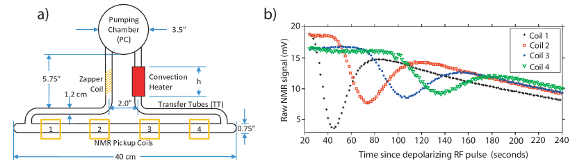
Figure 102: Shown in a) is the basic design for convection-based target cells, together with the instrumentation used to visualize gas flow. In b) NMR signals from the four pick-up coils are shown as a function of the time following the application of a depolarizing pulse of RF by the “zapper coil”. The dip in the signal from each coil marks the passage of a depolarized slug of gas.

3.17.2.1 Convection-based target cells and polarization gradients

The polarized ³He targets that have been used at JLab thus far are comprised of two chambers: 1) a pumping chamber in which the spin-exchange optical pumping takes place and 2) a target chamber through which the electron beam passes. Historically, these two chambers have been connected by a single “transfer tube”, and gas moved between the two chambers by diffusion. The polarization of the ³He in the target chamber, however, is determined by a balance between the rate at which it is being depolarized, and the rate at which it is being replenished with gas from the pumping chamber. At high luminosities, spin-relaxation due to the electron beam is quite significant, and diffusion between the two chambers becomes a bottleneck resulting in a significant “polarization gradient” between the pumping and target chambers. This problem would become quite severe at the higher luminosities planned for future experiments if no provision were made to address the issue.

The ratio of the equilibrium polarization in the target chamber, $P_{\mathrm{tc}}$ to the equilibrium polarization in the pumping chamber, $P_{\mathrm{pc}}$, is given by [16]

$${{P_{\mathrm{tc}}}\over{P_{\mathrm{pc}}}}={{1}\over{1+\Gamma_{\mathrm{tc}}/d_{\mathrm{tc}}}}$$ (52)

where $\Gamma_{\mathrm{tc}}$ is the spin-relaxation rate specific to the target chamber and $d_{\mathrm{tc}}$ is the rate at which atoms are leaving the target chamber. Clearly, it is important to keep the ratio $\Gamma_{\mathrm{tc}}/d_{\mathrm{tc}}\ll 1$, something that becomes more difficult as the beam current is increased.

Depolarization of polarized ³He in spin-exchange-based targets is well understood both experimentally [17] and theoretically [18]. For our conditions, the formula for the beam-induced spin-relaxation rate of ³He nuclei in a cylindrical target cell of cross-sectional area $A_{tc}$ is well approximated by:

$$\Gamma_{\mathrm{beam}}=\left(5\times 10^{-3}{{\rm cm^{2}}\over{\rm\mu A\,hr}}\right)I/A_{tc}\ \ ,$$ (53)

where $I$ is the current of the beam. Multiple comparisons with experimental data from both SLAC and JLab have provided confidence that this formula can be trusted at the level of 10–20%. A good example involves a target cell we will refer to as Brady, that was used during the most recent set of polarized ³He experiments at JLab. More specifically, Brady was to study both single [19] and double-spin [20] asymmetries in semi-inclusive deep inelastic scattering. Because these experiments used a transversely polarized target, they are referred to collectively as the Transversity experiments. Using dimensions and operational parameters discussed in [14] and [16], we can use Eq. 53 to compute the beam-induced relaxation rate in the target chamber (not averaged over the whole cell) to be $\rm\Gamma_{\mathrm{beam}}=1/32\,hrs$ at $\rm 12\mu A$, which incidentally, is in good agreement with what was deduced from the experimental data. Other contributions to relaxation in the target chamber during Transversity came from frequent AFP flips ($\rm\sim 1/60\,hrs$) and the cell’s intrinsic relaxation rate ($\rm\sim 1/20\,hrs$). Collectively, this resulted in a net relaxation rate in the target chamber, $\rm\Gamma_{\mathrm{tc}}\sim 1/10\,hrs$. For Brady, $d_{\mathrm{tc}}=0.72\,hr^{-1}$, and using Eq. 52, we find $P_{\mathrm{tc}}/P_{\mathrm{pc}}=0.88$. For $A_{1}^{n}$, if the cell Brady were used, a beam current of $45\,\mu A$ would be required to achieve the proposed luminosity. This would result in $\rm\Gamma_{\mathrm{beam}}=1/8.6\,hrs$, and a net $\Gamma_{\mathrm{tc}}=\rm 1/6\,hrs$, and an expected ratio $P_{\mathrm{tc}}/P_{\mathrm{pc}}=0.81$. The average polarization in the target chamber during Transversity was 55.4% [19]. Using this as a starting point, the polarization that one would expect at $45\,\mu A$ would be 48.4%. At the highest luminosities currently projected for approved experiments, the maximum in-beam polarization would be more like 38.4%.

We have developed a new target-cell design that addresses the problem of polarization gradients. The target cells still have two chambers as before, but rather than connecting these two chambers by a single “transfer tube”, the chambers are connected by two transfer tubes. With a single transfer tube, gas moves between the two chambers by diffusion. With two transfer tubes, one tube can be heated while leaving the other tube at room temperature, a condition that leads to convective flow. In fact, we have demonstrated that we can vary the flow rate of gas moving through the target chamber from just a few cm/min up to around 80 cm/min in a very reproducible manner [16]. The geometry of the cell is illustrated in Fig. 102a. In Fig. 102b, NMR signals are plotted as a function of time for the four pickup coils shown in Fig. 102a. The dips associated with the data from each coil are due to the passage of a slug of gas that was depolarized by the “zapper coil” at time zero.

When using a convection-based cell, even a modest flow rate of $\rm 6\,cm/s$ results in a value of $d_{\mathrm{tc}}=\rm 9\,hr^{-1}$ for a target chamber with a length of $\rm 40\,cm$. If a convection-based cell were used under the conditions during which the target cell Brady was run, all other parameters being equal, we would expect the ratio $P_{\mathrm{tc}}/P_{\mathrm{pc}}>0.98$ while in beam, and $P_{\mathrm{tc}}/P_{\mathrm{pc}}>0.99$ with no beam. Not only would this significantly increase the polarization of the gas in the target chamber, it would also have significant advantages for polarimetry, as will be discussed in the section on polarimetry. This is because an absolute calibration of NMR signals in the pumping chamber could be easily translated into an absolute calibration of NMR signals in the target chamber since the polarization in the two chambers would be nearly the same. Indeed, during calibrations, the flow rate could be substantially increased. At $\rm 60\,cm/s$, for example, under calibration conditions, we would expect $P_{\mathrm{tc}}/P_{\mathrm{pc}}>0.999$, which would greatly aid cross calibrations between the pumping and target chambers.

3.17.2.2 High luminosity and target size

Totally apart from the question of polarization gradients, there is also the question of how to maintain high cell-averaged polarization in the face of the depolarizing effects of the electron beam at high currents. The solution to this issue is that it is necessary to polarize ³He at a rate that is rapid compared to the rate at which it is being depolarized. Eq. 53 gives the beam-induced spin-relaxation rate in the target chamber. If instead we want to know the beam-induced spin-relaxation rate averaged over the entire cell, it can be written as

$$\rm\Gamma_{\mathrm{beam}}^{\mathrm{av}}=f_{\mathrm{tc}}\,\Gamma_{\mathrm{beam}}=f_{\mathrm{tc}}\,\left(5\times 10^{-3}{{\rm cm^{2}}\over{\rm\mu A\,hr}}\right)I/A_{tc}$$ (54)

where $f_{\mathrm{tc}}$ is the fraction of ³He atoms in the target chamber. If we want to make $\Gamma_{\mathrm{beam}}^{\mathrm{av}}$ small, we need to make $f_{\mathrm{tc}}$ small, which in turn means increasing the volume of the pumping chamber. For the Transversity target cell Brady considered earlier, $f_{\mathrm{tc}}=0.43$ under operating conditions, yielding $\rm\Gamma_{\mathrm{beam}}^{\mathrm{av}}=1/75\,hrs$. For $A_{1}^{n}$, however, where the beam current would need to be $\rm 45\,\mu A$ if we were to use Brady, $\rm\Gamma_{\mathrm{beam}}=1/8.6\,hrs$, and $\rm\Gamma_{\mathrm{beam}}^{\mathrm{av}}=1/20\,hrs$. To avoid having a lower cell-averaged polarization, we would need to use a pumping chamber with a larger volume.

In Fig. 103a, we show a target-cell geometry with two pumping chambers and a $\rm 60\,cm$ long target chamber for which we developed a relatively detailed oven design as well as magnetic-field calculations. Under operating conditions, $f_{\mathrm{tc}}=0.23$ for both this cell and the geometry shown in Fig. 103b. Using Transversity as a benchmark, these two double-pumping-chamber geometries can be expected to deliver over 60% polarization with a $\rm 60\,\mu A$ electron beam. Originally, we had hoped to use one of these two geometries for the Hall A $A_{1}^{n}$ experiment, which was proposed to run with a beam current of $\rm 30\,\mu A$. This plan would provide a considerable margin of safety, and provide valuable data so that the target design could be tweaked for subsequent higher-luminosity experiments. In fact, however, again using Transversity as a benchmark, the single-pumping-chamber geometry shown in Fig. 103c, which has a target-chamber length of $\rm 40\,cm$, should in principle be nearly adequate for Hall A $A_{1}^{n}$ if the beam current is increased to $\rm 45\,\mu A$ (to compensate for the shorter target chamber). This statement is relatively consistent with an optimistic interpretation of a simulated beam test we performed with Protovec-I, a cell whose geometry is quite close to that of Fig. 103c. As will be discussed shortly, a pessimistic interpretation of this same simulated beam test suggests that a target with the geometry of Fig. 103c would achieve 50% polarization, a performance level with an effective figure of merit around 2/3 of the proposal value.

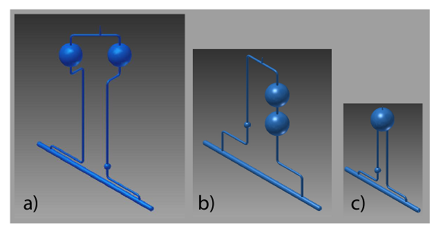
Figure 103: Shown are 3D renderings of three cell geometries that have been considered. In a) and b) there are two pumping chambers and the target chambers are $\rm 60\,cm$ in length. In c) there is one pumping chamber and the target chamber is $\rm 40\,cm$ in length. The geometry shown in c) is nearly identical to Protovec-I, bench tests of which are described in the text.

We describe next how to estimate the expected performance of the geometry shown in Fig. 103c using Transversity as a benchmark. The cell-averaged equilibrium polarization, $P_{\mathrm{He}}^{\mathrm{eq}}$, that any given target can achieve, can be written:

$$P_{\mathrm{He}}^{\mathrm{eq}}=\langle P_{\mathrm{alk}}\rangle{{\langle\gamma_{\mathrm{se}}\rangle}\over{\langle\gamma_{\mathrm{se}}\rangle(1+X)+\Gamma_{\mathrm{nx}}}}$$ (55)

where $\langle P_{\mathrm{alk}}\rangle$ is the average alkali polarization in the pumping chamber, $\langle\gamma_{\mathrm{se}}\rangle$ is the spin-exchange rate averaged over the cell, $X$ quantifies a spin-relaxation rate that is roughly proportional to $\langle\gamma_{\mathrm{se}}\rangle$, and $\Gamma_{\mathrm{nx}}$ is the spin relaxation due to everything other than spin exchange and the relaxation rate described by the parameter $X$. The ultimate polarization of a particular target is complicated by the fact that the parameter $X$ varies from cell to cell in a manner that is not understood, as is also the case with the wall-induced spin relaxation. We can proceed, however, by assuming that both $X$ and the wall relaxation are identical to the case of Brady for which $\rm\Gamma_{\mathrm{nx}}\sim 1/20\,hrs+1/75\,hrs+1/60\,hrs=1/12.5\,hrs$, where the first term was due to the “intrinsic” relaxation rate (a combination of wall relaxation and bulk relaxation due to ³He-³He collisions), the second term was due to the beam and the third term was due to the frequency of AFP spin flips that were used during Transversity. During $A_{1}^{n}$, it is reasonable to expect that the effective relaxation rate due to AFP measurements will be negligible. If we demand for some new target cell that $\rm\Gamma_{\mathrm{nx}}=1/12.5\,hrs$, as was the case for Brady during Transversity, and further assume a beam current of $\rm 45\,\mu A$, we are essentially demanding that

$$\rm\Gamma_{\mathrm{nx}}=1/12.5\,hrs=1/20\,hrs+f_{\mathrm{tc}}(1/8.6\,hrs)$$ (56)

which is satisfied if $f_{\mathrm{tc}}=0.26$. This value of $f_{\mathrm{tc}}$ is quite close to the value of 0.29 associated with the geometry of Fig. 103c. Indeed, we can probably adjust the design shown in Fig. 103c to make up the small difference.

The preceding argument suggests that the single-pumping-chamber geometry shown in Fig. 103c, which is extremely close to the geometry of the test cell Protovec-I, is cable of delivering 60% polarization at full luminosity. The argument is based on an extrapolation based on the proven performance achieved during Transversity. With that said, the argument also leaves no margin of safety, something that is of particular concern given that the $A_{1}^{n}$ target will be breaking new ground in several ways. We describe in the next section bench tests of Protovec-I which suggest that a target cell with the geometry shown in Fig. 103c is capable of achieving at least 50% polarization at full luminosity, and perhaps even higher polarization.

We return briefly to the cell geometries shown in Fig. 103a and b, both of which (due to their size and an extrapolation from Transversity such as that described above), can be expected to deliver polarization in excess of 60% at luminosities twice that of the Hall A $A_{1}^{n}$ experiment . We have developed in some detail certain aspects of a target-system design that could accommodate the geometry shown in Fig. 103a. These studies include magnetic-field calculations that are presented in their own section. More recently we have considered the advantages of the geometry shown in Fig. 103b, which due to the vertical stacking of the pumping chambers, can be pumped from almost any direction in the horizontal plane. For this reason, a vertically stacked geometry is practical for at least four of the approved polarized ³He experiments. Also, a vertically stacked geometry might reduce the magnetic field inhomogeneities experienced by the target for several of the magnet systems under consideration. The great success of the Hall A polarized ³He program has been due in part to the fact that the target designs, on paper, have always included a conservative margin of safety. The cell geometry shown in Fig. 103b would provide such a margin of safety for $A_{1}^{n}$, and would also be suitable for multiple polarized ³He experiments. All other things being equal, we view the vertically-stacked geometry of Fig. 103b as our preferred choice, and believe that it would be worthwhile to explore the question of whether pursuing its development sooner rather than later might ultimately prove to be the wisest choice, both in terms of cost and the success of the program.

3.17.2.3 Tests of Protovec-I

We have constructed two prototype target cells with geometries nearly identical to that shown in Fig. 103c and will refer to them as Protovec-I and Protovec-II. For Protovec-I, pictured in Fig. 104b, we have performed polarization tests in which we simulated the spin relaxation due to the electron beam by subjecting the cell to periodic pulses of RF. These RF pulses were applied to a small spherical volume that was situated along one of the two transfer tubes. The RF pulses tipped the nuclear spins of the ³He contained within that small volume so that they were at an angle of 90^∘ with respect to the magnetic holding field, causing them to precess and decay away. The same coil used to apply the pulses of RF was also used to detect the precessing spins, thus providing a measure of the polarization. The polarization as a function of time is shown in Fig. 104a, and is seen to saturate at 49%. We note further that the convection heater was set during these measurements to produce a gas velocity in the target chamber of $\rm 6\,cm/min$, which is the gas velocity at which we plan to run.

Figure 104: In a) we show a “spin-up”, polarization as a function of time while a target is being polarized. In b) we show a photograph of the cell being tested, Protovec-I. The polarization measurements shown in a) utilized pulse NMR, and the frequency of the RF pulses was chosen to simulate the depolarization that would result from a beam with a current in the range of $\rm 50-63\,\mu A$.

To the extent that we understand the polarization losses associated with the RF pulses, the data shown in Fig. 104a provide a measure of the expected performance of Protovec-I under running conditions. The uncertainty in the induced polarization losses are such that we believe we were simulating a beam current in the range of $\rm 50-63\,\mu A$. This was the first such test we have performed, and we expect to greatly reduce the uncertainties in the induced polarization losses in the future. We view these tests as a valuable tool for evaluating the expected performance of individual target cells under running conditions. For the test shown in Fig. 104a, a pessimistic interpretation suggests that Protovec-I is capable of achieving a polarization of 49% with roughly the beam current required to achieve full luminosity ($\rm 45\,\mu A$).

The simulated beam test shown in Fig. 104a is quite encouraging. The test was performed using only three lasers, whereas we expect to use four or five lasers when actually running. Furthermore, the measured properties of Protovec-I were not very good when compared with our better target cells. Brady, for example, was initially measured at UVa as having a spin-relaxation rate of less than $\rm 1/30\,hrs$, compared to just under $\rm 1/20\,hrs$ for Protovec-I. Also, the value of the $X$ parameter, while only measured roughly for Protovec-I, appeared significantly larger than that measured for Brady. In short, there are good reasons to expect that future simulated beam tests with new target cells will establish performance levels that exceed those achieved with Protovec-I. Even with no improvements, however, our tests suggest that a target such as Protovec-I would deliver an effective (polarization adjusted) luminosity of at least 2/3 of that which appears in the Hall A $A_{1}^{n}$ proposal.

3.17.2.4 Magnetic Field

The polarized ³He target uses a magnetic holding field that is typically on the order of $\rm 20\,G$. The current plan for the source of this magnetic field is to use the existing coils that were used for the Transversity experiment, although the question of whether these coils are adequate for the larger target cells that will be used for $A_{1}^{n}$ is not yet definitively answered. One design constraint is that magnetic field inhomogeneities need to be held to an acceptable level, something that is more challenging with a larger target volume. A second design issue is minimizing the deviation of the holding field direction from that which is desired, and in particular, controlling the vertical component of the magnetic field due to the fringe field of the BigBite dipole.

We present below the results of calculations performed using the program Tosca for two configurations, both of which are illustrated in Fig. 105. In both cases we assume that the field is produced using the two largest coils that were used during Transversity, and that both coils are oriented to produce a field whose direction is in the horizontal plane. In fact, the largest coil used during Transversity was used to produce field in the vertical direction, and orienting that coil to produce field in the horizontal direction would require new mounting hardware. At the time of this writing, the target system design being explored for $A_{1}^{n}$ would not use the largest of the three Transversity coils. For this and other reasons, the field studies presented here cannot be considered as being final. Nonetheless, they provide considerable insight as we proceed toward a final design.

In the first of the two configurations presented, shown in Fig. 105a, a single field clamp is used. In the second configuration presented, shown in Fig. 105b, two symmetric field clamps are used. Also, in this second configuration, two coils are wrapped around each of the two field clamps in order to energize them and produce a small vertical field to offset that due to the BigBite dipole.

Figure 105: Shown are two configurations whose magnetic field properties have been studied. In a), a single field clamp is used. In b), two symmetric field clamps are used, each of which is energized with two coils in order to produce a small vertical field to offset that due to the BigBite dipole.

One of the design criteria for the magnetic holding field is the longitudinal spin-relaxation rate, $1/T_{1}$, that is caused by magnetic field inhomogeneities. Since the magnetic field can have three components, and each component can have a non-zero derivative in three directions, the magnetic field inhomogeneities are described by a nine-component tensor. The longitudinal spin relaxation caused by magnetic field inhomogeneities under static conditions (as opposed to magnetic resonance conditions) is given by:

$${1\over{T_{1}}}={{|\vec{\nabla}B_{x}|^{2}+|\vec{\nabla}B_{y}|^{2}}\over{B_{z}^{2}}}D$$ (57)

where $\vec{B}$ is the static holding field, which is presumed here to be in the $z$ direction, and $D$ is the diffusion coefficient of the ³He [21]. For the configuration shown in Fig. 105a (single field clamp), when the field is along the beamline (the $z$ direction), we have used the program Tosca to compute the resulting magnetic field and show the magnitude of $B_{z}$ as a function of $z$ in Fig. 106a. Each point corresponds to values of $x$ and $y$ that are (for appropriate values of $z$) within one of the pumping chambers of the double-pumping-chamber cell geometry shown in Fig. 103a. Also shown, in Fig. 106b, is the quantity $(|\vec{\nabla}B_{x}|^{2}+|\vec{\nabla}B_{y}|^{2})^{1/2}$, the square of which appears in the numerator in Eq. 57.

Figure 106: For the vicinity of one of the pumping chambers of the cell depicted in Fig. 103a, and the single-field-clamp magnetic field configuration, we plot, as a function of $z$, the magnitude of the $z$ component of static holding field (a) and the indicated magnetic field inhomogeneities (b). The field direction is nominally along the beam-line direction, which is the $z$ axis.

In round numbers, we see that the inhomogeneities are of the order of $\rm 0.1\,G/cm$. For a 10 amagat sample of ³He, the diffusion constant $D\rm\sim 0.2\,cm^{2}/s$. This would result in $1/T_{1}\sim\rm 1/56\,hrs$, which in principle is tolerable, but would definitely cause some limitation to the polarization that would be achievable.

Another design criterion when considering the magnetic holding field are the polarization losses caused by magnetic field inhomogeneities during the NMR technique of adiabatic fast passage, or AFP, that we use for polarimetry. In this case, the losses are caused largely by $1/T_{1\rho}$, the longitudinal spin-relaxation rate in a frame that is rotating about the $z$ axis at the Larmor frequency. On resonance, this quantity is given by [22]

$${1\over{T_{1\rho}}}={{|\vec{\nabla}B_{z}|^{2}}\over{B_{1}^{2}}}D$$ (58)

where $B_{1}$ is the magnitude of the RF field, which is typically significantly smaller than the static holding field. The magnitude of the quantity ${|\vec{\nabla}B_{z}|}$ for the configuration shown in Fig. 105a is shown in Fig. 107 for a collection of points, again located inside one of the pumping chambers of the cell shown in Fig. 103a. It can be seen that the numbers span a considerable range, with an average that is, perhaps, somewhere around $\rm 0.075\,G/cm$. Using $B_{1}=\rm 0.05\,G$, a fairly typical value, we find the relaxation rate $1/T_{1\rho}=\rm 0.45\,s^{-1}$, much faster than before, but it only occurs during magnetic resonance conditions. Using the results of ref. [22], it can be shown that the fractional relaxation that occurs during AFP is well approximated by

$$\mathrm{fractional\ relaxation}={1\over{T_{1\rho}}}\,{{\pi\,B_{1}}\over{2(\partial B_{z}/\partial t)}}$$ (59)

where $\partial B_{z}/\partial t$ is the sweep rate of the magnetic holding field. Using $\partial B_{z}/\partial t=1.2\,\rm G/s$, we find a fractional loss of 0.029, or about 3%. In contrast, the same calculation for the case of $|\vec{\nabla}B_{z}|=20\,\rm mG/cm$ gives a loss of 0.21% (or 0.42% per polarization measurement), and for $|\vec{\nabla}B_{z}|=10\,\rm mG/cm$, a loss of 0.05%. In general, with the Hall A polarized ³He target, efforts have been made to keep inhomogeneities in the range of $\rm 10-20\,mG$, and the losses per polarization measurement (which involves two AFP spin flips), have generally been 0.5% or less, consistent with the predictions from Eq. 59.

If the AFP losses are truly 3% per spin flip, or 6% per polarization measurement, AFP cannot be used as the primary on-line monitor of polarization. It should still be possible to use pulse NMR polarimetry, however, by arranging to have the portion of the target cell being probed in a “sweet spot” with low field inhomogeneities.

Figure 107: For the configuration shown in Fig. 105a, with a single field clamp, we plot the magnitude of $\vec{\nabla}B_{z}$ in the vicinity of one of the pumping chambers of the cell depicted in Fig. 103a. The quantity $\vec{\nabla}B_{z}$ is a determining factor in the polarization losses that occur during the NMR technique of AFP. The inhomogeneities are seen to be significantly larger than the range of $\rm 10-20\,mG/cm$ that has typically been the goal when operating the Hall A polarized ³He target system.

As mentioned earlier, another design criterion that needs to be considered is the direction of the magnetic field. For $A_{1}^{n}$ this is not quite as critical as for some measurements (such as $G_{E}^{n}$), but it is still important. The fringe fields from the BigBite dipole are large, and in particular, there tends to be a significant unwanted vertical component in the field. Even when using a field clamp, as is the case in the configuration of Fig. 105a, there is still a significant vertical component, as is shown in Fig. 108a. By using two symmetrical field clamps, and energizing each with two coils (the configuration shown in Fig. 105b), the vertical component can be greatly reduced, as is shown in Fig. 108b. At the time of this writing, we are still studying the two-field-clamp configuration, but it certainly seems to have some advantages.

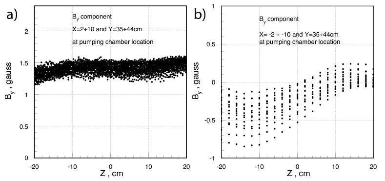
Figure 108: Shown is the vertical magnetic-field component, $B_{y}$, for points in the vicinity of one of the pumping chambers of the cell depicted in Fig. 103a. The plots a) and b) correspond to the single- and double-field-clamp configurations, respectively, depicted in Figs. 105a and b. The nominal magnetic-field direction is along the $z$ axis, which is parallel to the beam line.

The magnetic-field calculations presented above focused on locations that are relevant for a two-pumping-chamber design, and assumed that the magnetic field was being produced using the largest two of the three coils used during Transversity. In fact, however, the configuration that would be easiest and cheapest to implement would use the two smallest of the three coils used during Transversity. Using smaller coils almost certainly means larger gradients at equivalent locations. On the other hand, a single-pumping-chamber geometry allows for a more symmetric placement of the target cell, which may well mean that the target cell would experience smaller gradients, even when using the smaller coils. This question can only be answered by performing additional Tosca calculations.

In summary, the calculations presented above seem to suggest that a magnetic field generated using coils from the Transversity setup will suffice for $A_{1}^{n}$, although more calculations are needed to confirm this statement. The calculations also seem to indicate that we are likely to have gradients a bit larger than would be ideal. It is thus essential that we complete our calculations using Tosca as soon as possible, since the Hall A designers are already beginning to work on a detailed design for the target system. In parallel, we are also undertaking additional studies, both theoretical and experimental, on the effects of inhomogeneities on polarization losses while performing AFP. These studies are already underway, and will better define the levels of inhomogeneities that are tolerable.

3.17.2.5 Polarimetry

The online monitoring of polarization for the $A_{1}^{n}$ polarized ³He target will be accomplished using one or both of two NMR techniques. Historically, in the Hall A polarized ³He target system, the NMR technique of AFP has been used, and provides very precise and reproducible measurements. One drawback of AFP is that it requires reversing the orientation of all of the spins within the target, something that is problematic if some portions of the target are made out of metal (which blocks the RF). This would be the case, for instance, if we used metal end windows on the target chamber, something that we are actively developing. AFP would also be problematic if large parts of the target experienced excessive magnetic field inhomogeneities. The second polarimetry technique being considered is based on pulse NMR. In this technique the spins within a small region of the target cell are tipped from the direction of the holding field, and subsequently precess, resulting in what is often called a free induction decay, or FID. We routinely use pulse NMR for polarimetry at UVa, and it was this technique that was used to measure polarization during the simulated beam test that is presented in Fig. 104. Pulse NMR polarimetry has the advantage that it can be performed on a small well-localized region of the cell, which can be chosen to be well away from any parts of the cell that are made of metal, an in a region of the magnetic field that is sufficiently homogeneous. Pulse NMR polarimetry has the disadvantage, however, that we currently only trust it at the 5–10% level, which is not yet sufficient for the $A_{1}^{n}$ experiment. There are no obvious obstacles, however, to refining pulse NMR polarimetry so that it can be trusted at the level of several percent.

In discussing polarimetry, it is important to distinguish between the measurements that will monitor the target polarization on an ongoing basis, and the measurements that will calibrate those measurements. One technique for determining the absolute ³He polarization is the observation of polarization-induced frequency shifts in the electron paramagnetic resonances associated with the alkali vapors [23]. This can only be performed in the pumping chamber, however, even though the quantity of interest is the polarization in the target chamber. It is thus important to understand the ratio of the polarization in the target chamber to the polarization in the pumping chamber, $P_{\mathrm{tc}}/P_{\mathrm{pc}}$, which is given by Eq. 52. In the past, the uncertainty in $P_{\mathrm{tc}}/P_{\mathrm{pc}}$ has led to a 1-2% contribution to the relative uncertainty in polarimetry. In convection-based targets, however, this uncertainty can be reduced to a fraction of a percent, well below the level of most other sources of error in the polarimetry system.

To better understand the source of polarimetry errors associated with polarization gradients, we consider again the cell Brady used during the Transversity experiment. To compute $P_{\mathrm{tc}}/P_{\mathrm{pc}}$ using Eq. 52, we need to know both $d_{\mathrm{tc}}$, which for Brady was $\rm(0.72\pm 0.10)hr^{-1}$ and $\Gamma_{\mathrm{tc}}$. Ideally, the calibration of the NMR system would be done in the absence of beam, which would also typically mean the absence of the rapid polarization reversals that were used during Transversity running. The room-temperature spin-relaxation rate for Brady was measured at JLab to be $\rm 1/20\,hr$, and if we take this as the value for $\Gamma_{\mathrm{tc}}$, we find $P_{\mathrm{tc}}/P_{\mathrm{pc}}=0.935$. The quantity $\Gamma_{\mathrm{tc}}$ is not measured directly, however. It is really only the cell-averaged relaxation rate that is known with accuracy. The uncertainty in $\Gamma_{\mathrm{tc}}$ thus leads to something like a 1–2% uncertainty in $P_{\mathrm{tc}}/P_{\mathrm{pc}}$, and hence in the target polarization.

The situation is dramatically different in a convection based cell. We are planning to run our convection-based cells at a gas velocity of $\rm 6\,cm/hr$, which as discussed earlier, results in a value of $d_{\mathrm{tc}}=\rm 9\,hr^{-1}$ for a target chamber with a length of $\rm 40\,cm$. If we again take $\Gamma_{\mathrm{tc}}=\rm 1/20\,hr$, we have $P_{\mathrm{tc}}^{\infty}/P_{\mathrm{pc}}^{\infty}=0.994$. Even large changes in the assumed value of $\Gamma_{\mathrm{tc}}$ would change this number by at most a few tenths of a percent. Furthermore, when actually performing a calibration, faster gas velocities would be used, resulting in uncertainties of well under $0.1\%$.

The above discussion has important implications for the strategy we will employ for polarimetry. Historically, AFP signals in the target chamber have been compared to AFP signals from thermally polarized water contained in a glass cell with a geometry that is similar, but not identical, to that of the target cells. To compare the water signals to the ³He signals, one must also take into account geometric factors, such as the slightly different size of the two chambers, and their placement in the NMR pickup coils. One of the most thorough such comparisons was done by Michael Romalis [24], during the experiment E154 at SLAC [25]. The error in this comparison was quoted as being 1.6%. Even if one did twice this well, it would still dwarf the error with which the quantity $P_{\mathrm{tc}}/P_{\mathrm{pc}}$ is known. Thus, during $A_{1}^{n}$, there is no advantage in obtaining water signals from the location of the target chamber, and this will not be attempted. Calibration of ³He signals with thermally polarized water will still be made, either directly or indirectly, but these comparisons will be obtained under more optimal conditions.

3.17.2.6 Mechanical aspects of the $A_{1}^{n}$ target

At the time of this writing, the design of the mechanical aspects of the Hall A $A_{1}^{n}$ target system is only just beginning. The strategy that is currently being explored involves using as much of the hardware developed for Transversity as possible. The oven, which will accommodate a convection-based cell, will necessarily be different, as will the placement of the coils, which must accommodate the planned kinematics. Many other aspects of the hardware, however, will be be either partially or fully reused. Examples include the support and drive mechanisms for the oven/target ladder, the laser and optics, the support structure for the Helmholtz coils, and many aspects of the polarimetry system. The primary reason for reusing as much as possible the Transversity hardware is to keep costs down.

A considerable amount of effort has gone into developing a conceptual design for the $A_{1}^{n}$ target that goes beyond what might best be described as an adaptation of the Transversity target. The primary reason for this is to accommodate a double-pumping-chamber cell of the sort shown in Figs. 103a and b. The cell pictured in Fig. 103b, with vertically stacked pumping chambers, has the distinct advantage that it can be pumped from almost any direction that falls in the horizontal plane, making it practical for at least four of the planned polarized ³He experiments. It could even be fitted with an oven that could rotate about a vertical axis, thus obviating the need to build a custom oven for each experiment. We have spent some time considering the advantages of mounting the cell and oven assembly on a frame that would be supported from the bottom, thus making weight less of an issue. There is little doubt that such a system would be more expensive than our current strategy in the short term. When considering all the experiments that such a system could serve, however, it may actually be cheaper than adapting the existing Transversity hardware.

Regardless of whether we use a single or double pumping chamber, and regardless of many other details of the target system, an important innovation in the $A_{1}^{n}$ polarized ³He target will be the inclusion of radiation shielding between the pumping chamber and the target chamber. When target cells have exploded during running, it is usually after prolonged exposure to the beam, and a reasonable assumption is that the target has suffered weakening due to radiation damage. It is usually the pumping chamber that ruptures, and this is presumably because the stresses in the relatively large pumping chamber are larger than those associated with the smaller-diameter target chamber. It is thus reasonable to expect that providing radiation shielding for the pumping chamber would make it possible to substantially increase the integrated luminosity over which the targets can be used. Radiation shielding is not practical for non-convecting target cells because the pumping and target chambers must be kept relatively close to one another. In a convection-driven cell, however, the distance between the pumping and target chambers can be quite large, making it practical for the first time to shield the pumping chamber.

An important question that is currently open regarding mechanical aspects of the target is whether there will be metal end windows on the target chamber. This is particularly relevant because the current design being explored would utilize a single-pumping-chamber cell with a target chamber that is $\rm 40\,cm$ in length instead of $\rm 60\,cm$, as in the original proposal. With the shorter target cell, full luminosity would only be achieved by using a $\rm 45\mu A$ beam instead of the proposed value of $\rm 30\mu A$. While we are fairly confident that glass end windows will tolerate a $\rm 30\mu A$ beam (this has actually been briefly tested), it is less clear that glass end windows will tolerate a $\rm 45\mu A$ beam. We are currently developing a design for beryllium end windows, but the approach has not yet been fully validated. Thus, achieving full luminosity with a $\rm 40\,cm$ long target chamber may be contingent on the success of our metal-end-window development work.

3.17.2.7 Target Design Summary

It is useful to list a few selected conclusions from our conceptual design for the Hall A $A_{1}^{n}$ target.

• The use of a convection-style target cell will be essential to achieving high polarization.

• A double-pumping chamber target cell can be expected to comfortably achieve the performance assumed in the proposal.

• A single-pumping-chamber cell may not achieve the desired polarization of over 60% at the proposed high luminosity. A polarization over 50% seems fairly likely.

• A single-pumping chamber cell can be mechanically accommodated by modifying the existing Transversity target hardware.

• Achieving full luminosity with a target cell that has a single pumping chamber and a $\rm 40\,cm$ target chamber may be contingent on the successful development of suitable metal end windows.

• The magnetic-field calculations that have been performed thus far show magnetic field inhomogeneities that would make online AFP polarimetry impossible. The configurations considered, however, do not correspond to the design currently being considered, so more calculations are needed.

• Pulse NMR polarimetry may be necessary if either 1) parts of the target cell are made of metal, or 2) is the magnetic field inhomogeneities are too large for performing AFP frequently.

• The absolute calibration of the polarimetry system can take advantage of the fact that the polarizations in the pumping and target chambers are nearly equal in a convection-driven cell. One consequence of this is that there is no advantage to studying signals from thermally polarized water at the location of the target chamber.

From the bullet points listed above, we conclude that a credible path forward exists that would make maximal use of existing hardware from Transversity, and that would achieve a figure of merit at least 2/3 of what was assumed in our proposal. Risks associated with this plan include some uncertainty as to whether suitable metal end windows can be constructed, and the possible need to use pulse NMR polarimetry for online monitoring of the polarization. The target assumed in the original proposal, which is larger and would probably have two pumping chambers, would almost certainly deliver the full figure of merit assumed in the proposal. It would share both of the risks mentioned above, and it would be more expensive. Such a target, however, might need only limited modification to be used for at least three experiments other than the Hall A $A_{1}^{n}$ experiment.

3.17.3 Summary

The A1n collaboration is working in close contact with the SBS collaboration, which will use the BigBite for several experiments.

The new timing hodoscope for BigBite consists of 90 25$\times 25\times 600$ mm bars of plastic scintillator. It is currently under construction. Tests of an element of the hodoscope, in conjunction with the NINO card, have been made using cosmic rays. The mean pulse height and mean time from readout of the 2 PMT attached to a hodoscope bar is close to position independent. The time difference of the PMTs gives a horizontal position resolution of $\sim 4.5$ cm. The vertical position resolution is set by the 25 mm lateral dimension of the bar. The time resolution is $\sim 0.4$ ns. This is possibly limited by the type ELT9125 PMTs which will be used for the A1n experiment. For an inclusive $(e,e^{\prime})$ measurement such as A1n, this level of time resolution is entirely adequate. However for a coincidence $(e,e^{\prime}n)$ measurement, such as in the $G_{M}^{n}$ experiment, improved resolution may be desirable. The hodoscope bars will also be tested with alternative PMTs with faster rise time. We also envisage testing of the NINO card and hodoscope elements under high intensity conditions at Mainz.

The NINO chip gives good timing performance with photomultiplier signals. Its time over threshold logic signal is an effective alternative to a pulse amplitude measurement in correcting for time walk in the discriminator. The tests described here relate to a scintillator hodoscope, but the NINO card will also be suitable for the BigBite gas Cerenkov counter GRINCH.

3.18 E12-07-108 - $G_{M}^{p}$

Precision Measurement of the Proton Elastic Cross Section at High $Q^{2}$

J. Arrington, M. Christy, S. Gilad, B. Moffit, V. Sulkosky and B. Wojtsekhowski, spokespersons,

and

the Hall A collaboration.

contributed by V. Sulkosky and B. Wojtsekhowski, for the GMp collaboration.

The GMp experiment was proposed to measure the elastic electron-proton cross-section from 7 to 17 GeV² in $Q^{2}$ with an unprecedented precision of less than 2%. The experiment has two main goals. The first goal is a precise measurement of the proton elastic cross-section at the kinematics of the upgraded JLab 12 GeV facility for accurate normalization of other experiments. The second objective is to determine with improved precision the proton magnetic form-factor $G_{M}^{p}$ at high $Q^{2}$. The JLab PAC recommended a beam time assignment of 24 days by asking the experimentalists not to pursue measurements at the two highest Q² points, which limits the highest planned $Q^{2}$ to 14 GeV².

The GMp and DVCS [1] experiments are scheduled to be the first two experiments to run after the 12 GeV upgrade in Hall A. The tentative plan is to concurrently run the two experiments to the greatest extent possible. The GMp collaboration is working in close contact with the DVCS collaboration, which will use the left high resolution spectrometer (HRS). Since the approval of the proposal, the collaboration has made a significant step in the instrumentation preparation which is briefly presented below.

3.18.1 Electron beam quality requirements

To achieve the goals outlined above, the GMp experiment requires the highest beam energy possible after the upgrade, $\sim$ 11 GeV into Hall A. The $Q^{2}$ range is achieved by using three standard beam energies (6.6 GeV, 8.8 GeV and 11 GeV) and two non-standard energies at 4.8 GeV and 5.8 GeV. These later two energies are necessary to study the $\epsilon$ dependence in order to constrain two photon exchange (TPE) corrections.

Of concern for the experiment is the accuracy of the beam energy. The current plan is to use the ARC energy method, which has provided a precision of (3–4)$\times$10^-4. The ARC energy system is in the process of being upgraded for the 12 GeV beam. After the upgrade, the system will be recalibrated using elastic scattering from hydrogen and tantalum targets with 2.2 GeV incident electrons. The beam stability and energy spread will be monitored by using the Optical Transition Radiation viewer, Synchrotron Light Interferometer and Tiefenback energy readback, the latter which is based on the beam positions from the beam position monitors (BPMs) located in the Hall A arc.

The incident beam angle can be determined by using the BPMs located near the target in Hall A with an uncertainty of 0.1 mrad. The beam charge is typically known to $\pm$0.5% with careful monitoring and calibration of the beam current monitors.

3.18.2 Detector configuration of the HRS spectrometers

The detector configuration, shown in Fig. 109, includes the vertical drift chambers (VDCs), the S0 and S2m counters, the Gas Cherenkov, the lead glass calorimeter, and one of the front FPP chambers. The last is an existing detector used many times in the left HRS. It is the only non-standard item in an otherwise traditional electron arm configuration. By using this chamber, we plan to resolve a long-standing problem of HRS tracking analysis whose efficiency of track reconstruction is less than 95% in spite of a high chamber efficiency of 99.5%. For the VDCs, the amplifier/discriminator (A/D) cards are in the process of being replaced with those developed for the BigBite wire chambers [2]. These new cards use MAD chips [3], whose output stage works with LVDS signals, which produce significantly less feedback than ECL signals used in A/D cards by LeCroy Research Systems. This allows the VDCs to be operated at lower discriminator thresholds and high voltages. The status of these detectors is presented in Section 3.18.2.

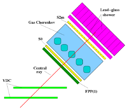
Figure 109: The planned detector configuration for the left and right HRSs for GMp with three wire chambers.

For the spectrometer optics calibration, a sieve-slit placed at the entrance to the spectrometers will be used to calibrate the solid angle acceptance, and carbon foils will be used along the beam line to calibrate the vertex position.

3.18.3 Configuration of the target

The standard Hall A cryogenic target ladder will be used with a liquid hydrogen target and carbon and aluminum solid targets for spectrometer optics calibrations and target background measurements, respectively. The thickness of the hydrogen target needs to be well defined. We plan to use 15 cm LH₂ “race-track” style cells that feature vertical flow of cryogenic fluid to reduce the effects of target density fluctuations. Earlier experiments used 20-cm long race-track cells.

3.18.3.1 Vertical-flow liquid hydrogen cell and performance

In 2002, tests had shown that the standard cigar-shaped cells displayed large density fluctuations with liquid hydrogen even with moderate beam currents at high fan speeds and large raster sizes. For this reason, the race-track cell [4] with vertical fluid flow was designed and built by the Cal State LA group in coordination with the JLab target group for the HAPPEx-II and HAPPEx-He experiments [5]. With the new race-track cells, the density fluctuations for an LH2 target were an order of magnitude smaller under similar raster sizes and fan speeds compared to the standard cells. The collaboration determined that with a 5 mm $\times$ 5 mm raster size that density fluctuations would contribute negligibly for a hydrogen target at 100 $\mu$A. However, during the 2005 run period, the fan speed had to be increased from the nominal 60 Hz to 91 Hz to minimize the density fluctuations. We plan to perform a detailed study of the density fluctuations from the race-track cell during commissioning of the experiment.

3.18.4 Swing arm wire target

Accurate knowledge of the scattering angle is very important in the GMp experiment. However, the mechanical stability of the Hall A spectrometers has a known problem, which could lead to a several mm displacement of the vertex. Regular checks of the spectrometer pointing by using the optics target mounted on the long ladder of the cryo-target provide an indication of stability but are insufficient for the level of accuracy needed in the GMp experiment. We have proposed a solution to this problem by using a tungsten wire target mounted on the scattering chamber via a short arm, see Fig. 110.

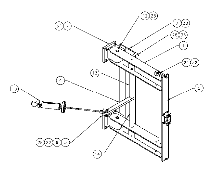
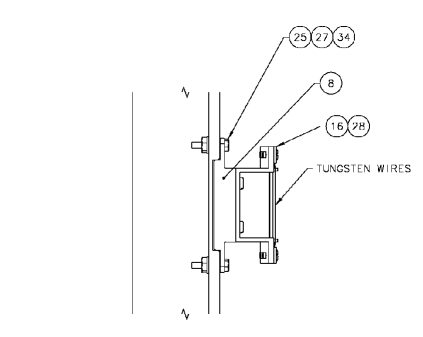
Figure 110: Shown is a schematic view of the swing arm target. The right-hand side figure illustrates the tungsten wires that will be placed in the beam.

3.18.5 Systematic Uncertainty and Expected Results

Achieving the total expected precision on the cross-section measurement requires serious work to minimize the systematic uncertainties on several parameters. Some of the most critical include the scattering angle, detector efficiencies, deadtime, spectrometer acceptance, target density and beam charge. A few of these items were discussed in the previous sections. The contributions to the total uncertainty expected on the differential cross section are summarized in Table 14.

Source	$\Delta\sigma/\sigma$ (%)
Point to Point uncertainties
Incident Energy	$<$0.3
Scattering Angle	0.1–0.3
Incident Beam Angle	0.1–0.2
Radiative Corrections*	0.3
Beam Charge	0.3
Target Density Fluctuations	0.2
Spectrometer Acceptance	0.4–0.8
Al Endcap Subtraction	0.1
Detector efficiencies and dead time	0.3
quadratic sum	0.8–1.1
Normalization uncertainties
Beam Charge	0.4
Target Thickness/Density	0.5
Radiative Corrections*	0.4
Spectrometer Acceptance	0.6–1.0
Al Endcap Subtraction	0.1
Detector efficiencies and dead time	0.4
quadratic sum	1.0–1.3
Statistics	0.5–0.8
Total (Scale+Rand.+Stat.)	1.2–1.7
* Not including two photon exchange

Table 14: GMp expected systematic uncertainties on the cross section.

In Figure 111, the published world data on the form factor $G^{p}_{M}$ versus $Q^{2}$ is shown along with the range and uncertainties for the expected results of the planned experiment.

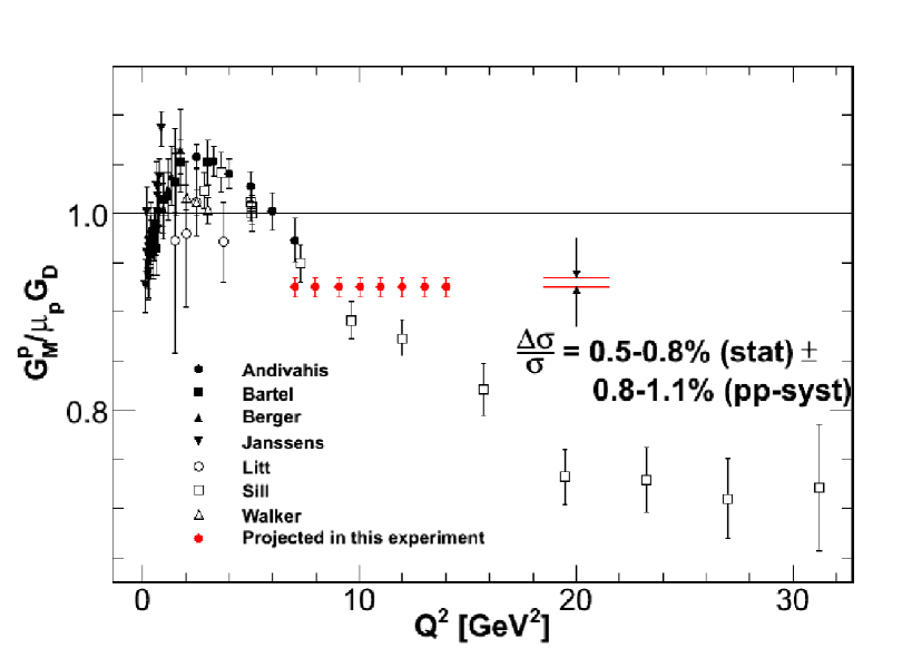
Figure 111: Published world data (Refs. [6, 7, 8, 9, 10, 11, 12]) for $G^{p}_{M}/\mu_{p}G_{D}$ as a function of $Q^{2}$, and the expected results for the proposed measurements. The uncertainties do not include the normalization uncertainty.

3.18.6 Summary

For the GMp experiment, we aim to measure the proton elastic cross section for $Q^{2}$ = 7–14 GeV² with a total precision of less than 2%. A few additional general purpose devices and improved analysis techniques will be used to aid our understanding of the systematic uncertainties. The precision of these measurements will greatly benefit other measurements of the proton form factors that rely on the proton cross section, and this measurement will also provide an extraction of $G_{M}^{p}$, which is needed for accurate determination of $G_{E}^{p}$ from future polarization transfer measurements.

4 Publications

1. O. Glamazdin, Moeller (iron foils) existing techniques, Nuovo Cimento C035N04, 176(2012)

2. H. Fonvieille et al., Virtual Compton Scattering and the Generalized Polarizabilities of the Proton at $Q^{2}=0.92$ and 1.76 GeV², Phys. Rev. C86, 015210 (2012)

3. S. Abrahamyan et al., Measurement of the Neutron Radius of ²⁰⁸Pb Through Parity-Violation in Electron Scattering, Phys. Rev. Lett. 108, 112502 (2012)

4. Z. Ahmed et al., New Precision Limit on the Strange Vector Form Factors of the Proton, Phys. Rev. Lett. 108, 102001 (2012)

5. J. Huang et al., Beam-Target Double Spin Asymmetry $A_{LT}$ in Charged Pion Production from Deep Inelastic Scattering on a Transversely Polarized He-3 Target at $1.4<Q^{2}<2.7$ GeV², Phys. Rev. Lett. 108, 052001 (2012)

6. A. Puckett et al., Final Analysis of Proton Form Factor Ratio Data at $Q^{2}=$ 4.0, 4.8 and 5.6 GeV², Phys. Rev. C85, 045203 (2012)

7. M. Mihovilovic et al., Methods for Optical Calibration of the BigBite Hadron Spectrometer, Nuclear Instruments & Methods 686, 20 (2012)

8. S. Abrahamyan et al., New Measurements of the Transverse Beam Asymmetry for Elastic Electron Scattering from Selected Nuclei, Phys. Rev. Lett. 109, 192501 (2012)

9. M. Friend, et al., Upgraded photon calorimeter with integrating readout for the Hall A Compton polarimeter at Jefferson Lab. Nuclear Instruments & Methods A 676, 96 (2012)

10. D.S. Parno, et al., Comparison of Modeled and Measured Performance of GSO Crystal as Gamma Detector. arXiv:1211.3710 [physics.ins-det]

5 Theses

1. Polarized ${}^{3}\mathrm{He}(e,e^{\prime}n)$ Asymmetries in Three Orthogonal Measurements
   Elena Long, Kent State
   http://arxiv.org/abs/1209.2739

2. Measurement of double polarized asymmetries in quasi-elastic processes ${}^{3}\vec{He}(\vec{e},e^{\prime}d)$ and ${}^{3}\vec{He}(\vec{e},e^{\prime}p)$
   Miha Mihovilovic, University of Ljublijana
   http://arxiv.org/abs/1208.0748

3. Precision Measurement of Electroproduction of $\pi^{0}$ near Threshold
   Khem Chirapatpimol, University of Virginia
   https://userweb.jlab.org/~khem/thesis/thesis.pdf

4. Probing Novel Properties of Nucleons and Nuclei via Parity Violating Electron Scattering
   Luis Mercado, University of Massachusetts, Amherst
   http://scholarworks.umass.edu/cgi/viewcontent.cgi?article=1588&context=open_access_dissertations

5. Probing the Strangeness Content of the Proton and the Neutron Radius of ²⁰⁸Pb using Parity-Violating Electron Scattering
   Rupesh Silwal, University of Virginia
   http://hallaweb.jlab.org/experiment/HAPPEX/silwal_thesis.pdf

6. A Precision Measurement of the Proton Strange-Quark Form Factors at $Q^{2}=0.624$ GeV²
   Megan Friend, Carnegie Mellon University
   http://www-meg.phys.cmu.edu/~mfriend/onlinethesis.pdf

7. Measurement Of Neutron Radius In Lead By Parity Violating Scattering Flash ADC DAQ
   Zafar Ahmed, Syracuse University
   http://surface.syr.edu/phy_etd/120/

6 Hall A Collaboration Member List

Argonne National Lab
John Arrington
Frank Dohrmann
Paul Reimer
Jaideep Singh
Xiaohui Zhan

Budker Institute of Nuclear Physics
Dima Nikolenko
Igor Rachek

Cairo University
Hassan Ibrahim

California Institute of Technology
Xin Qian

California State University
Konrad A. Aniol
Martin B. Epstein
Dimitri Margaziotis

Carnegie Mellon University
Gregg Franklin
Vahe Mamyan
Brian Quinn

The Catholic University of America
Tanja Horn

Commissariat a l’Energie Atomique - Saclay
Maxime Defurne

China Institute of Atomic Energy (CIAE)
Xiaomei Li
Shuhua Zhou

Christopher Newport University
Ed Brash

College of William and Mary
David S. Armstrong
Todd Averett
Juan Carlos Cornejo
Melissa Cummings
Wouter Deconinck
Keith Griffioen
Joe Katich
Lubomir Pentchev
Charles Perdrisat
Huan Yao
Bo Zhao

Dapnia/SphN
Nicole d’Hose
Franck Sabatie

Duquesne University
Fatiha Benmokhtar

Duke University
Steve Churchwell
Haiyan Gao
Calvin Howell
Min Huang
Simona Malace
Richard Walter
Qiujian Ye

Faculte des Sciences de Monastir (Tunisia)
Malek Mazouz

Florida International University
Armando Acha
Werner Boeglin
Luminiya Coman
Marius Coman
Lei Guo
Hari Khanal
Laird Kramer
Pete Markowitz
Brian Raue
Jeorg Reinhold

The George Washington University
Ramesh Subedi

Gesellschaft fur Schwerionenforschung (GSI)
Javier Rodriguez Vignote

Hampton University
Eric Christy
Leon Cole
Ashot Gasparian
Peter Monaghan

Harvard University
Richard Wilson

Hebrew University of Jerusalem
Moshe Friedman
Aidan Kelleher
Guy Ron

Huangshan University
Hai-jiang Lu
XinHu Yan

Idaho State University
Mahbub Khandaker
Dustin McNulty

INFN/Bari
Raffaele de Leo

INFN/Catania
Vincenzo Bellini
Sutera Concetta Maria
Antonio Guisa
Francesco Mammoliti
Giuseppe Russo
Maria Leda Sperduto

INFN/Lecce
Roberto Perrino

INFN/Roma
Marco Capogni
Francesco Cusanno
Alessio Del Dotto
Salvatore Frullani
Franco Garibaldi
Franco Meddi
Guido Maria Urciuoli
Evaristo Cisbani
Rachel di Salvo
Mauro Iodice

Institut de Physique Nucleaire
Alejandro Marti Jimenez-Arguello

Institute of Modern Physics, Chinese Academy of Sciences
Xurong Chen

Institut de Physique Nucleaire - Orsay
Camille Desnault
Rafayel Paremuzyan

ISN Grenoble
Eric Voutier

James Madison University
Gabriel Niculescu
Ioana Niculescu

Jefferson Lab
Kalyan Allada
Alexandre Camsonne
Larry Cardman
Jian-Ping Chen
Eugene Chudakov
Kees de Jager
Alexandre Deur
Ed Folts
David Gaskell
Javier Gomez
Ole Hansen
Douglas Higinbotham
Mark K. Jones
Thia Keppel
John Lerose
Bert Manzlak
David Meekins
Robert Michaels
Bryan Moffit
Sirish Nanda
Noel Okay
Andrew Puckett
Yi Qiang
Lester Richardson
Yves Roblin
Brad Sawatzky
Jack Segal
Dennis Skopik
Patricia Solvignon
Mark Stevens
Riad Suleiman
Stephanie Tysor
Bogdan Wojtsekowski
Jixie Zhang

Jozef Stefan Institute
Miha Mihovilovic
Simon Sirca

Kent State University
Bryon Anderson
Mina Katramatou
Elena Khrosinkova
Elena Long
Richard Madey
Mark Manley
Gerassimos G. Petratos
Larry Selvey
Andrei Semenov
John Watson

Kharkov Institute of Physics and Technology
Oleksandr Glamazdin
Viktor Gorbenko
Roman Pomatsalyuk
Vadym Vereshchaka

Kharkov State University
Pavel Sorokin

Khalifa University
Issam Qattan

Lanzhou University
Bitao Hu
Yi Zhang

Longwood University
Tim Holmstrom
Keith Rider
Jeremy St. John
Wolfgang Troth

Los Alamos Laboratory
Jin Huang
Xiaodong Jiang
Ming Xiong Liu

LPC Clermont-Ferrand France
Pierre Bertin
Helene Fonvielle
Carlos Munoz Camacho

Mississippi State University
Dipangkar Dutta
Mitra Shabestari
Amrendra Narayan
Nuruzzaman

Massachusetts Institute of Technology
Bill Bertozzi
Shalev Gilad
Navaphon “Tai” Muangma
Kai Pan
Cesar Fernandez Ramirez
Rupesh Silwal
Vincent Sulkosky

Negev Nuclear Research Center
Arie Beck
Sharon Beck

NIKHEF
Jeff Templon

Norfolk State University
Vina Punjabi

North Carolina Central University
Benjamin Crowe
Branislav (Branko) Vlahovic

Northwestern University
Ralph Segel

Ohio University
Julie Roche

Old Dominion University
Gagik Gavalian
Mohamed Hafez
Wendy Hinton
Charles Hyde
Hashir Rashad
Larry Weinstein

Peterburg Nuclear Physics Institute
Viacheslav Kuznetsov

Regina University
Alexander Kozlov

Rutgers University
Lamiaa El Fassi
Ron Gilman
Gerfried Kumbartzki
Katherine Myers
Ronald Ransome
Yawei Zhang

Saint Norbert College
Michael Olson

Seoul National University
Seonho Choi
Byungwuek Lee

Smith College
Piotr Decowski

St Mary’s University
Davis Anez Adam Sarty

Stanford Linear Accelerator
Rouven Essig

Syracuse University
Zafar Ahmed
Richard Holmes
Paul A. Souder

Tel Aviv University
Nathaniel Bubis
Or Chen
Igor Korover
Jechiel Lichtenstadt
Eli Piasetzky
Ishay Pomerantz
Ran Shneor
Israel Yaron

Temple University
David Flay
Eric Fuchey
Zein-Eddine Meziani
Michael Paolone
Matthew Posik
Nikos Sparveris

Tohoku University
Kouichi Kino
Kazushige Maeda
Teijiro Saito
Tatsuo Terasawa
H. Tsubota

Tsinghua University
Zhigang Xiao

Universidad Complutense de Madrid (UCM)
Joaquin Lopez Herraiz
Luis Mario Fraile
Maria Christina Martinez Perez
Jose Udias Moinelo

Universitat Pavia
Sigfrido Boffi

University “La Sapienza” of Rome
Cristiano Fanelli
Fulvio De Persio

University of Glasgow
John Annand
David Hamilton
Dave Ireland
Ken Livingston
Dan Protopopescu
Guenther Rosner
Johan Sjoegren

University of Illinois
Ting Chang
Areg Danagoulian
J.C. Peng
Mike Roedelbronn
Youcai Wang
Lindgyan Zhu

University of Kentucky
Dan Dale
Tim Gorringe
Wolfgang Korsch

University of Lund
Kevin Fissum

University of Manitoba
Juliette Mammei

University of Maryland
Elizabeth Beise

University of Massachusetts, Amherst
Krishna S. Kumar
Seamus Riordan
Jon Wexler

University of New Hampshire
Toby Badman
Trevor Bielarski
John Calarco
Greg Hadcock
Bill Hersman
Maurik Holtrop
Donahy John
Mark Leuschner
James Maxwell
Sarah Phillips
Karl Slifer
Timothy Smith
Ryan Zielinski

University of Regina
Garth Huber
George Lolos
Zisia Papandreou

University of Saskatchewan
Ru Igarashi

University of Science and Technology of China (USTC)
Yi Jiang
Wenbiao Yan
Yunxiu Ye
Zhengguo Zhao
Yuxian Zhao
Pengjia Zhu

University of South Carolina
Steffen Strauch

University of Virginia
Khem Chirapatpimol
Mark Dalton
Donal Day
Xiaoyan Deng
Gordon D. Gates
Gu Chao
Charles Hanretty
Ge Jin
Sudirukkuge Tharanga Jinasundera
Richard Lindgren
Jie Liu
Nilanga Liyanage
Vladimir Nelyubin
Blaine Norum
Kent Paschke
Peng Chao
Oscar Rondon
Kiadtisak Saenboonruang
William “Al” Tobias Diancheng Wang
Kebin Wang
Zhihong Yi
Zhiwen Zhao
Xiaochao Zheng
Jiayao Zhou

University of Washington
Diana Parno

Yamagata University
Seigo Kato
Hiroaki Ueno

Yerevan Physics Institute
Sergey Abrahamyan
Nerses Gevorgyan
Edik Hovhannisyan
Armen Ketikyan
Samvel Mayilyan
Artush Petrosyan
Galust Sargsyan
Albert Shahinyan
Hakob Voskanian

Past Members
Mattias Anderson
Maud Baylac
Hachemi Benaoum
J. Berthot
Michel Bernard
Louis Bimbot
Tim Black
Alexander Borissov
Vincent Breton
Herbert Breuer
Etienne Burtin
Christian Cavata
George Chang
Nicholas Chant
Jean-Eric Ducret
Zhengwei Chai
Brandon Craver
Natalie Degrande
Pibero Djawotho
Chiranjib Dutta
Kim Egiyan
Stephanie Escoffier
Catherine Ferdi
Megan Friend
Robert Feuerbach
Mike Finn
Bernard Frois
Oliver Gayou
Charles Glashausser
Jackie Glister
Brian Hahn
Harry Holmgren
Sebastian Incerti
Riccardo Iommi
Florian Itard
Stephanie Jaminion
Steffen Jensen
Cathleen Jones
Lisa Kaufman
James D. Kellie
Sophie Kerhoas
Ameya Kolarkar
Norm Kolb
Ioannis Kominis
Serge Kox
Kevin Kramer
Elena Kuchina
Serguei Kuleshov
Jeff Lachniet
Geraud Lavessiere
Antonio Leone
David Lhuillier
Meihua Liang
Han Liu
Robert Lourie
Jacques Marroncle
Jacques Martino
Kathy McCormick
Justin McIntyre
Luis Mercado
Brian Milbrath
Wilson Miller
Joseph Mitchell
Jean Mougey
Pierre Moussiegt
Alan Nathan
Damien Neyret
Stephane Platchkov
Thierry Pussieux
Gilles Quemener
Abdurahim Rakhman
Bodo Reitz
Rikki Roche
Philip Roos
David Rowntree
Gary Rutledge
Marat Rvachev
Arun Saha
Neil Thompson
Luminita Todor
Paul Ulmer
Antonin Vacheret
Luc Van de Hoorebeke
Robert Van de Vyver
Pascal Vernin
Dan Watts
Krishni Wijesooriya
Hong Xiang
Wang Xu
Jingdong Yuan
Jianguo Zhao
Jingdong Zhou
Xiaofeng Zhu
Piotr Zolnierczuk

References

- [1] Glamazdin A.V., Gorbenko V.G., Levchuk L.G. et.al. Electron Beam Møller Polarimeter at JLab Hall A. FizikaB (Zagreb) V. 8. 1999, pp. 91-95.
- [2] Ken Bagget. Private communication.
- [3] O. Glamazdin. Moeller (iron foils) existing techniques. Nuovo Cim. C035 N04. 2012, pp. 176-180.
- [4] E. Chudakov, O. Glamazdin, R. Pomatsalyuk. Møller Polarimeter, Configuration #2. Hall A Annual report 2010. pp.10-18.
- [5] P. Steiner, A. Feltham, I. Sick, et. al. A high-rate coincidence Moller polarimeter. Nucl.Instrum.Methods. A419. 1998. pp. 105-120.
- [6] G.G. Scott. Magnetomechanical Ratios for Fe-Co Alloys. Phys.Rev. V. 184. 1969. pp. 490-491.
- [7] B. Sawatzky, Z. Ahmed, C-M Jen, E. Chudakov, R. Michaels, D. Abbott, H. Dong, E. Jastrzembski. Møøller FADC DAQ Upgrade. Hall A Annual report 2009. pp.25-30.
- [8] B. Sawatzky, Z. Ahmed, C-M Jen, E. Chudakov, R. Michaels, D. Abbott, H. Dong, E. Jastrzembski. Møller FADC DAQ upgrade. Internal Review. Jefferson Lab, December, 2010, p. 7.

References

- [1] S. Nanda and D. Lhuiellier, Conceptual Design Report for Hall A Compton Polarimeter Upgrade, Unpublished.
- [2] G. Bardin et.al, Conceptual Design Report of a Compton Polarimeter for Cebaf Hall A, CEA, Saclay, France, Unpublished.
- [3] Jlab Experiment E06002, Paul Souder, Robert Michaels, Guido Urciuoli spokespersons.
- [4] S. Nanda, Conceptual Design Report for Hall A Compton Polarimeter 12 GeV Upgrade, Unpublished.
- [5] M. Bregant et al., arXIV:hep-ex/0202046 v1 28 Feb 2002.
- [6] Innolight GmbH, http://www.innolight.de/
- [7] IPG Photonics, http://www.ipgphotonics.com/
- [8] HC Photonics, http://www.hcphotonics.com/
- [9] Advanced Thin Films, http://www.atfilms.com/
- [10] Joly et al. , Tests of an electron detector system with cosmic muons for JLab Hall A Compton polarimeter, Universite Blaise Pascal, Clermont-Ferrand report.
- [11] Fang Jun, Shanghai Institute of Ceramics, http://www.siccas.com/
- [12] Jay Benesch et al., Reducing Synchrotron Radiation in the Compton Photon Detector, Hall A Collaboration Meeting, June 7-8, 2012. pdf

References

-
[1]
https://hallaweb.jlab.org/wiki/index.php/Hall_A_He3_Polhe3_Target;
Y. Zhang, et al., Nucl. Instru. Meth. A, to be submitted. - [2] M. Amarian et al., Phys. Rev. Lett. 89, 242301 (2002); 92, 022301 (2004); 93, 152301 (2004); Z. Meziani,et al., Phys. Lett. B 613, 148 (2005).
- [3] W. Xu, et al., Phys. Rev. Lett. 85, 2900 (2000); F. Xiong, et al., Phys. Rev. Lett. 87, 242501 (2001).
- [4] X. Zheng, et al., Phys. Rev. Lett.92, 012004 (2004); Phys. Rev. C 70, 065207 (2004).
- [5] K. Kramer, et al., Phys. Rev. Lett. 95, 142002 (2005).
- [6] P. Solvignon, et al., Phys. Rev. Lett. 101, 182502 (2008).
- [7] JLab E97-110, Spokespersons, J. P. Chen, A. Deur and F. Garibaldi.
- [8] S. Riordan et al., Phys. Rev. Lett. 105, 262302 (2010).
- [9] X. Qian et al., Phys. Rev. Lett. 107, 072003 (2011); J. Huang et al., Phys. Rev. Lett. 108, 052001 (2012).
- [10] JLab E07-013, Spokespersons, T. Averett, T. Holmstrom and X. Jiang.
- [11] JLab E06-014, Spokespersons, S. Choi, X. Jiang, Z.-E. Meziani, B. Sawatzky.
- [12] JLab E05-015, Spokespersons, T. Averett, J. P. Chen and X. Jiang.
- [13] JLab E05-102, Spokespersons, S. Gilad, D. Higinbotham, W. Korsch, B. Norum, S. Sirca.
- [14] JLab E08-005, Spokespersons, T. Averett, D. Higinbotham and V. Sulkosky.
- [15] K. Slifer, PhD thesis, Temple University (2004).
- [16] X. Zheng. PhD thesis, MIT (2002).
- [17] W. Happer et al., U.S. Patent No. 6,318,092 2001; E. Babcock, et al., Phys. Rev. Lett. 91, 123003 (2003).
- [18] A. Ben-Amar Baranga, S. Appelt, M.V. Romalis, C.J. Erickson, A.R. Young, G.D. Cates and W. Happer, Polarization of by Spin Exchange with Optically Pumped Rb and K Vapors, Phys. Rev. Lett. 80, 2801 (1998).
- [19] Jaideep Singh, Ph.D. thesis, University of Virginia (2010).
- [20] M.V. Romalis, PhD thesis, Princeton University (1998).
- [21] Y. Zhang, PhD thesis, Lanzhou University (2011).
- [22] JLab E12-10-006, Spokespersons, J. P. Chen, H. Gao, , X. Jiang, J. C. Peng and X. Qian; JLab E12-11-007, Spokespersons, J. P. Chen, J. Huang, X. Li, Y. Qiang and W. Yan.
- [23] JLab E12-06-122, Spokespersons, T. Averett, G. Cates, N. Liyanage, G. Rosner, B. Wojtsekhowski and X. Zheng.
- [24] JLab E12-06-121, Spokespersons, T. Averett, W. Korsch, Z.-E. Meziani, B. Sawatzky.
- [25] JLab E12-09-018, Spokespersons, G. Cates, E. Cisbana, G. Franklin, A. Puckett and B. Wojtsekhowski.
- [26] JLab E12-06-110, Spokespersons, G. Cates, J. P. Chen. Z.-E. Meziani and X. Zheng.
- [27] JLab E12-09-016, Spokespersons, G. Cates, S. Riordan and B. Wojtsekhowski.
- [28] P.A.M. Dolph, J. Singh, T. Averett, A. Kelleher, K.E. Mooney, V. Nelyubin, W.A. Tobias, B. Wojtsekhowski and G.D. Cates, Gas dynamics in high-luminosity polarized targets using diffusion and convection, Phys. Rev. C 84, 065201 (December 2010).

References

- [1] The Podd home page at http://hallaweb.jlab.org/podd/
- [2] Details at http://scicomp.jlab.org/disk/volatile.faces

References

- [1] J. Alcorn et al., Nucl. Instrum. Meth. A522 (2004) 294-346.
- [2] Hall A annual report 2007, page 13-15.
- [3] J. Arrington, B. Moffit, S. Gilad, E. Christy, V. Sulkovsky, B. Wojtsekhowski (contact). ” Precision Measurement of the Proton Elastic Cross-Section at High Q2”, Jefferson Lab experiment E12-07-108.
- [4] Hall A annual report 2002, page 31-34.
- [5] ELJEN Technology, http://www.eljentechnology.com.
- [6] Hall A annual report 2004, page 22-24.
- [7] Hamamatsu, http://jp.hamamatsu.com/en/index.html.

References

- [1] Hall A annual report 2004, page 22-24.
- [2] Hamamatsu, http://jp.hamamatsu.com/en/index.html.

References

- [1] D. Hamilton et al., NIM A 643, 1 (2011).
- [2] D. Hamilton et al., Phys. Rev. Lett. 94, 242001 (2005).
- [3] A. Danagoulian et al., Phys. Rev. Lett. 98, 152001 (2007).
- [4] A. Danagoulian, PhD Thesis (2006).

References

- [1] M.O. Distler et al., Phys. Rev. Lett. 80, 2294 (1988).
- [2] H. Merkel et al., Phys. Rev. Lett. 88, 12301 (2002).
- [3] D. Drechsel, S.S. Kamalov and L. Tiator, Eur. Phys. J. A34, 69 (2007).
- [4] H. Merkel et al., ”Proceedings of the 6th International Workshop on Chiral Dynamics July 6-10 2009, Bern, Switzerland”.
- [5] S.S. Kamalov and S.N. Yang, Phys. Rev. Lett. 83, 4494 (1999).
- [6] http://wwwkph.kph-uni-mainz.de/MAID//dmt/dmt2001.html.
- [7] K. Wang et al., computer code, private communication.
- [8] J. Heisenberg, computer code, private communication.
- [9] E.A.J.M. Offerman et al., Phys. Rev. C44, 1096 (1991).

References

- [1] E.Babcock et al., Phys. Rev. Lett. 91, 123003 (2003).
- [2] J.Alcorn et al., Nucl. Inst. Meth. 522, 294 (2004).
- [3] X.Zheng et al., (Jefferson Lab Hall A Collaboration), Phys. Rev. Lett. 92, 012004 (2004).

References

- [1] S. Širca, S. Gilad, D. W. Higinbotham, W. Korsch, B. E. Norum (spokespersons), Measurement of and asymmetries in the quasi-elastic , TJNAF Experiment E05-102.
- [2] M. Mihovilovič et al. (Hall A Collaboration), Methods for optical calibration of the BigBite hadron spectrometer, Nucl. Instr. Meth. A 686 (2012) 20.

References

- [1] S. Wandzura and F. Wilczek, Phys. Lett. B 72, 2 (1977).
- [2] R.L. Jaffe, Comm. Nucl. Part. Phys. 19, 239 (1990).
- [3] B.W. Filippone and Xiandong Ji, Adv. Nucl. Phys. 26, 1 (2001). arXiv:0101224v1 [hep-ph].
- [4] M. Burkardt, The Spin Structure Function (2009), arXiv:0905.4079v1 [hep-ph].
- [5] M. Burkardt, Parton Distributions in the Impact Parameter Space (2008), arXiv:0902.0163v1 [hep-ph].
- [6] S. Choi, X. Jiang, Z.-E. Meziani, B. Sawatzky et al., Jefferson Lab PAC E06-014 (2005).
- [7] M. Gockeler et al., Phys. Rev. D 72, 054507 (2005).
- [8] P. Solvignon, private communication.
- [9] E.V. Shuryak and A.I. Vainshtein, Nucl. Phys. B 201, 141 (1982).
- [10] Ji and Chou, Phys. Rev. D 42, 3637 (1990).
- [11] M. Amerian et al., Phys. Rev. Lett. 89, 242301 (2002).
- [12] K. Slifer et al., Resonance Spin Structure, 2008. arXiv:0812.0031.
- [13] D. Drechel, S.S. Kamolov and L. Tiatar, Eur. Phys. J. A34, 69 (2007).
- [14] P.L. Anthony et al., Phys. Lett. B 553, 18 (2003).
- [15] N. Isgur, Phys. Rev. D 59, 0340123 (1999).
- [16] K. Abe et al., SLAC-PUB-7753 (Feb. 1998).
- [17] K. Abe et al., Phys. Rev. Lett. 79, 26 (1997); Phys. Lett. B 405, 180 (1997).
- [18] K. Ackerstaff et al., Phys. Lett. B 404, 383 (1997).
- [19] X. Zheng et al., Phys. Rev. C 70, 065207 (2004).
- [20] E. Leader, A.V. Siderov, D.B. Stamenov, Int. J. Mod. Phys A13, 5573 (1998).
- [21] J.P. Ralson, P. Jain, R.V. Buniy, AIP Conf. Proc. 549, 302 (2000).
- [22] K.V. Dharmawardane et al., Phys. Lett. B 641, 11 (2006).
- [23] G. Cates, N. Liyanage, Z.-E. Meziani, G. Rosner, B. Wojtsekhowski, X. Zheng et al., Jefferson Lab PAC E1206122 (2006).
- [24] G. Cates, J.P. Chen, Z.-E. Meziani, X. Zheng et al., Jefferson Lab PAC E1210101 (2010).
- [25] J.L. Friar et al.,Phys. Rev. C 42, 6 (1990).
- [26] F. Bissey, A.W. Thomas and I.R. Afnan, Phys. Rev. C 64, 024004 (2001).
- [27] M. Anselmino et al., Phys. Rep. 261, 1–124 (1995).
- [28] D. Parno, Ph.D. Thesis, Carnegie Mellon University (2011).
- [29] I. Kominis, Ph.D. Thesis, Princeton University (2001).
- [30] J. Singh, A Note About Beam Depolarization, Univeristy of Virginia (2008).
-
[31]
M. Posik et al., E06-014 Analysis Status Report 2011,
https://hallaweb.jlab.org/wiki/images/8/8c/D2n_HallAReport_2011_v5.pdf - [32] L.W. Mo and Y.S. Tsai, Rev. Mod. Phys. 40, 205 (1969).
- [33] R. Altulmus and J. Wise, rosetail.f, fortran analysis code.
- [34] S. Stein et al., Phys. Rev. D 12, 1884 (1975).
- [35] Roy Whitney, radcor.f, fortran analysis code.
- [36] P.E. Bosted and V. Mamyan, Empirical Fit to electron-nucleus scattering (2012), arXiv:1203.2262v2 [nucl-th].
- [37] P.L. Anthony et al., Phys. Rev. D 54, 6620 (1996).
- [38] P. Solvignon et al., Phys. Rev. Lett. 101, 182502 (2008).
- [39] F. Bissey et al., Phys. Rev. C 65, 064317 (2002).
- [40] S.A. Kulagin and W. Melnitchouk, Phys. Rev. C 78, 065203 (2008).
- [41] D. de Florian, R. Sassot, M. Stratmann, W. Vogelsang, Global Analysis of Helicty Parton Densities and Their Uncertainties, arXiv:0804.0422 [hep-ph].
- [42] H. Weigel, L. Gamberg and H. Reinhart, Phys. Rev. D 55, 6910 (1997).
- [43] C.R.V. Bourrely, J. Soffer and F. Buccella, Eur. Phys. J. C 41, 327 (2005) [arXiv:hep-ph/0502180].
- [44] M. Stratmann, Z. Phys. C 60, 763 (1993).
- [45] K. Kramer et al., Phys. Rev. Lett. 95, 142002 (2005).

References

- [1] S. Gilad, D. Higinbotham, E. Piasetzky, V. Sulkosky and J. Watson (spokespersons) JLab experiment E07-006 (2007).
- [2] R. Subedi et al., Science 320 (2008) 1476.
- [3] M. Mihovilovic et al., Nucl. Instrum. Meth. 686 (2012) 20.
- [4] R.A. Cecil et al., Nucl. Instrum. Meth. 161 (1979) 439.

References

- [1] S. V. Goloskokov and P. Kroll, Eur. Phys. J. A 47, 112 (2011) [arXiv:1106.4897 [hep-ph]].
- [2] C. M. Camacho et al. [Jefferson Lab Hall A and Hall A DVCS Collaborations], Phys. Rev. Lett. 97 (2006) 262002 [nucl-ex/0607029].
- [3] F. Feinstein [ANTARES Collaboration], Nucl. Instrum. Meth. A 504, 258 (2003).

References

- [1] R. Pohl et al., Nature 466, 213 (2010).

References

- [1] Glister J. et al., Nucl. Instr. and Meth. in Phys. Research A. V.606 I.3 2009. P.578–584 (arXiv:0904.1493)
- [2] Zhan X., “High Precision Measurement of the Proton Elastic Form Factor Ratio at Low ”, Doctoral Thesis, MIT 2010

References

- [1] J.R. Vignote, private communication
- [2] F. Benmokhtar et al. Phys. Rev. Lett. 94 082305

References

- [1] A. de Rujula, H. Georgi and S.L. Glashow et al., Phys. Rev D12, 147 (1975).
- [2] N. Isgur, G. Karl and R. Koniuk, Phys. Rev. D25, 2394 (1982); S. Capstick and G. Karl, Phys. Rev. D41, 2767 (1990).
- [3] G. Blanpied et al., Phys. Rev. Lett. 79, 4337 (1997).
-
[4]
R. Beck et al., Phys. Rev. Lett. 78, 606 (1997);
ibid. 79, 4515 (1997) (Erratum).
R. Beck et al., Phys. Rev. C61, 35204 (2000). - [5] V.V. Frolov et al., Phys. Rev. Lett. 82, 45 (1999).
- [6] T. Pospischil et al., Phys. Rev. Lett. 86, 2959 (2001).
- [7] C. Mertz et al., Phys. Rev. Lett. 86, 2963 (2001).
- [8] P. Bartsch et al., Phys. Rev. Lett. 88, 142001 (2002).
- [9] L.D. van Buuren et al., Phys. Rev. Lett. 89, 12001 (2002).
- [10] N.F. Sparveris et al., Phys. Rev. Lett. 94, 022003 (2005).
- [11] J.J. Kelly et al., Phys. Rev. Lett. 95, 102001 (2005).
- [12] N.F. Sparveris et al., Phys. Lett. B 651, 102 (2007).
- [13] S. Stave et al., Eur. Phys. J. A 30, 471 (2006).
- [14] D. Elsner et al., Eur. Phys. J. A 27 91-97 (2006).
- [15] K. Joo et al., Phys. Rev. C68, 032201 (2003); K. Joo et al., Phys. Rev. C70, 042201 (2004)
- [16] S. Stave, N. Sparveris et al., Physical Review C78, 025209 (2008)
- [17] M. Ungaro et al., Phys. Rev. Lett. 97, 112003 (2006).
- [18] A. N. Villano et al., Phys. Rev. C 80, 035203 (2009)
- [19] I.G. Aznauryan et al. Phys. Rev. C 80, 055203 (2009)
- [20] C. Alexandrou et al., Phys. Rev D83 014501 (2011); Phys. Rev. Lett. 94, 021601 (2005).
- [21] T. Sato and T.-S.H. Lee, Phys. Rev. C63, 055201 (2001).
- [22] S.S. Kamalov and S. Yang, Phys. Rev. Lett. 83, 4494 (1999)
- [23] S.S. Kamalov et al., Phys. Lett. B 522, 27 (2001).
- [24] D. Drechsel et al., Nucl. Phys. A 645, 145 (1999).
- [25] D. Drechsel and L. Tiator, J. Phys. G18, 449 (1992)
- [26] R.A. Arndt, et al. Phys. Rev. C66, 055213 (2002); nucl-th/0301068 and http://gwdac.phys.gwu.edu
- [27] V. Pascalutsa and M. Vanderhaegen et al., Phys. Rev. Lett. 95, 232001 (2005) and V. Pascalutsa and M. Vanderhaegen et al., Phys. Rev. D73, 034003 (2006).
- [28] A.M. Bernstein, Eur. Phys. J. A 17, 349 (2003).
- [29] S.L. Glashow, Physica A 96, 27 (1979)
- [30] D.H. Lu, A.W. Thomas, A.G. Williams, Phys. Rev. C55, 3108 (1997); U. Meyer, E. Hernandez, A.J. Buchmann, Phys. Rev. C64, 035203 (2001); M. Fiolhais, B. Golli, S. Sirca, Phys. Lett. B 373, 229 (1996)
- [31] T. A. Gail and T. R. Hemmert, Eur. Phys. J. A 28 (1), 91-105 (2006)

References

- [1] C.Y. Prescott et al., Phys. Lett. B77, 347 (1978).
- [2] C.Y. Prescott et al., Phys. Lett. B84, 524 (1979).
- [3] L.W. Mo and Y.-S. Tsai, Rev. Mod. Phys. 41, 205 (1969).
- [4] K. Matsui, T. Sato and T.-S. H. Lee, Phys. Rev. C72, 025204 (2005).
- [5] M. Gorchtein, C.J. Horowitz, and M. Ramsey-Musolf, Phys. Rev. C84, 015502 (2011).
- [6] J. Pumplin et al., JHEP 07, 012 (2002).
- [7] H.-L. Lai, M. Guzzi, J. Huston, Z. Li, P.M. Nadolsky et al., Phys. Rev. D82, 074024 (2010).
- [8] A.D. Martin, W.J. Stirling, R.S. Thorne, G. Watt, Phys. Lett. B652, 292 (2007).
- [9] A.D. Martin, W.J. Stirling, R.S. Thorne, G. Watt, Eur. Phys. J. C63, 189 (2009).

References

- [1] L. Lapikas, Nucl. Phys. A553, 297c (1993).
- [2] L.L. Frankfurt, M.I. Strikman, D.B. Day, M. Sargsian, Phys. Rev. C 48, 2451 (1993).
- [3] R. Shneor et al, Phys. Rev. Lett. 99, 072501 (2007).
- [4] P. Solvignon, J. Arrington, D.B. Day, D. Higinbotham et al., Jefferson Lab experiment E12-11-112.
- [5] N. Fomin et al, Phys. Rev. Lett. 108 092502 (2012).
- [6] K.S. Egiyan et al, Phys. Rev. Lett. 96, 082501 (2006).
- [7] P. Solvignon, J. Arrington, D.B. Day, D. Higinbotham et al., Jefferson Lab experiment E08-014.
- [8] L.L. Frankfurt, M. Sargsian, M.I. Strikman, Int. J. Mod. Phys. A23 2991-3055 (2008).
- [9] M. Martini et al, Phys. Rev. C 80 065501 (2009).

References

- [1] F. R. Wesselmann et al. [RSS Collaboration], Phys. Rev. Lett. 98, 132003 (2007).
- [2] R. Pohl et al., Nature 466, 213 (2010).
- [3] M. Amarian et al. [Jefferson Lab E94010 Collaboration], Phys. Rev. Lett. 93, 152301 (2004).
- [4] V. Bernard, T. R. Hemmert and U. G. Meissner, Phys. Lett. B 545, 105 (2002).
- [5] C. W. Kao, T. Spitzenberg and M. Vanderhaeghen, Phys. Rev. D 67, 016001 (2003).

References

- [1] Hall A annual report 2004, page 22-24.
- [2] Hamamatsu, http://jp.hamamatsu.com/en/index.html.
- [3] F. Anghinolfi, et al., Nucl. Instr. and Meth. A533, 183 (2004).
- [4] N. Liyanage, University of Virginia, using fits and models for pion production cross sections, 2011.
-
[5]
B. Sawatzky, Hall A Technical Note for the Bigbite Cherenkov Detector,
https://jlabdoc.jlab.org/docushare/dsweb/Get/Document-61783/12-038.pdf. - [6] U. Akgun et al., (2010) JINST 5 P08005.
- [7] V. Nelyubin, “A GEANT Simulation of Background Rate in Quartz Window of PMT XP4508 in Cherenkov Detector”, (2011).
- [8] B. Wojtsekhowski, private communication (2012).
- [9] E. Cisbani et al., Nucl. Inst. Meth. A496 (2003) 305.
- [10] I. Adam et al., Nucl. Inst. Meth. A538 (2005) 281.
- [11] P. Bourgeois and J. Va’vra, “Corrosion of Glass Windows in DIRC PMTs”, Technical Report (date, post BaBar).
- [12] E. Jensen, “Testing DIRC PMTs”, (2012); and private communication.
- [13] W. Happer, G. Cates, M. Romalis, and C. Erikson, U.S. patent no. 6318092 (2001); E. Babcock, I. Nelson, S. Kadlecek, B. Driehuys, L. W. Anderson, F. W. Hersman, and T. G. Walker, Phys. Rev. Lett. 91, 123003 (2003).
- [14] Jaideep Singh, P.A.M. Dolph, W.A. Tobias, T. Averett, A. Kelleher, K.E. Mooneyz, V. Nelyubin, Yunxiao Wang, Yuan Zheng, and G.D. Cates, The Development of High-Performance Alkali-Hybrid Polarized Targets for Electron Scattering. We plan to submit this manuscript to Phys. Rev. C shortly. and a near-final draft is available on a local UVa server which can be found at: http://people.virginia.edu/~gdc4k/hybrid_prc_v14.pdf.
- [15] B. Wojtsekhowski, “Prospect for Measuring GEn at High Momentum Transfers”, in Newport News 2002, Exclusive Processes At High Momentum Transfer (edited by A. Radyushkin, P. Stoler; Singapore, World Scientific, 2002, pp 273-281.
- [16] P.A.M. Dolph, J. Singh, T. Averett, A. Kelleher, K. E. Mooney, V. Nelyubin, W.A. Tobias, B. Wojtsekhowski and G. D. Cates, Gas dynamics in high-luminosity polarized targets using diffusion and convection, Phys. Rev. C 84, 065201 (December 2011).
- [17] K.P. Coulter, A.B. McDonald, G.D. Cates, W. Happer, and T.E. Chupp, Measurement of 3He depolarization rates during bombardment with a 4He beam, Nucl. Inst. and Meth. in Phys. Res. A276, 29 (1989).
- [18] K. D. Bonin, T. G. Walker, and W. Happer, Relaxation of gaseous spin-polarized 3He targets due to ionizing radiation, Phys. Rev. A 37, 3270 (1988).
- [19] X. Qian et al., Single Spin Asymmetries in Charged Pion Production from Semi-Inclusive Deep Inelastic Scattering on a Transversely Polarized Target at , Phys. Rev. Lett. 107, 072003 (2011).
- [20] J. Huang et al., Beam-Target Double Spin Asymmetry in Charged Pion Production from Deep Inelastic Scattering on a Transversely Polarized Target at , Phys. Rev. Lett. 108, 052001 (2012).
- [21] G.D. Cates, S. Schaefer, and W. Happer, Relaxation of Spins due to Field Inhomogeneities in Gaseous Samples at Low Magnetic Fields and Low Pressures, Phys. Rev. A 37, 2877 (1988).
- [22] G.D. Cates, D. J. White, Ting-Ray Chien, S.R. Schaefer, and W. Happer, Spin Relaxation in gases due to inhomogeneous static and oscillating magnetic fields, Phys. Rev. A 38, 5092 (1988).
- [23] M.V. Romalis and G.D. Cates, Accurate 3He polarimetry using the Rb Zeeman frequency shift due to the Rb-3He spin-exchange collisions, Phys. Rev. A 58, 3004 (1998).
- [24] M. Romalis, Ph.D. Thesis, Princeton University (1997).
- [25] K. Abe et al. (the SLAC E-154 collaboration), Precision Determination of the Neutron Spin Structure Function , Phys. Rev. Lett. 79, 26 (1997).

References

- [1] C. Hyde, B. Michel, C. Munoz Camacho, J. Roche et al., Jefferson Lab experiment E12-06-114.
- [2] B. Wojtsekhowski, R. Lindgren, and N. Liyanage, Hall A Status Report 2006 (2007) 16.
- [3] M. Pegoraro, Proceedings of the Fourth Workshop on Electronics for LHC Experiments, CERN/LHCC/98-36, (1998) 257.
- [4] J.-P. Chen and D. Armstrong, Hall A Status Report 2004 (2005) 20.
- [5] A. Acha et al., Phys. Rev. Lett. 98 (2007) 032301.
- [6] L. Andivahis et al., Phys. Rev. D50 (1994) 5491.
- [7] W. Bartel et al., Nucl. Phys. B58 (1973) 429.
- [8] C. Berger, V. Burkert, G. Knop, B. Langenbeck, and K. Rith, Phys. Lett. B35 (1971) 87.
- [9] T. Janssens, R. Hofstadter, E. B. Hughes, and M. R. Yearian, Phys. Rev. 142 (1966) 922.
- [10] J. Litt et al., Phys. Lett. B31 (1970) 40.
- [11] R. C. Walker et al., Phys. Rev. D49 (1994) 5671.
- [12] A. F. Still et al., Phys. Rev. D48 (1993) 29.