Shape effects on localized surface plasmon resonances in metallic nanoparticles

Abstract

The effect of smooth shape changes of metallic nanoparticles on localized surface plasmon resonances is assessed with a boundary integral equation method. The boundary integral equation method allows compact expressions of nanoparticle polarizability which is expressed as an eigenmode sum of terms that depends on the eigenvalues and eigenfunctions of the integral operator associated to the boundary integral equation method. Shape variations change not only the eigenvalues but also their coupling weights to the electromagnetic field. Thus rather small changes in the shape may induce large variations of the coupling weights. It has been found that shape changes that bring volume variations greater than 12% induce structural changes in the extinction spectrum of metallic nanoparticles. Also the largest variations in eigenvalues and their coupling weights are encountered by shape changes along the smallest cross-sections of nanoparticles. These results are useful as guiding rules in the process of designing plasmonic nanostrucrures.

I Introduction

Localized surface plasmon resonances (LSPRs) have their origin in the interaction of metallic nanoparticles (NPs) with light. The advancements made in the last decade have enabled the use of LSPRs for light manipulation at the nanoscale Halas (2010). The applications of LSPRs include enhanced sensing and biosensors Nie and Emory (1997); Kabashin et al. (2009), cancer imaging and therapy Loo et al. (2005), plasmonic lasers Hill and et al. (2007) and spasers Stockman (2008), enhanced nonlinearities, etc. Metallic NPs can be made by chemical synthesis or by lithographic techniques. Thus a large variety of shapes have been obtained by chemical synthesis. Beside the spheres, the shapes include nanorods Yu et al. (1997), cubes El-Sayed (2001); Sau and Murphy (2004), triangular prisms Okada et al. (2004), tetrahedra El-Sayed (2001), and hexagonal prisms Sau and Murphy (2004). In contrast, in “top-down” or lithographic techniques the shape of the metallic NPs are “flatter” such that structures like disks Haynes et al. (2003), dimers of disks Rechberger et al. (2003) or bowtie structures Fromm et al. (2004) have been successfully fabricated.

Optical properties associated with LSPRs are determined by the shape, size, structure, and local dielectric environment of the NPs Kelly et al. (2003); c. F. Bohren and Huffman (1998). Along with the electric field enhancement created around NPs, the effect of the dielectric surrounding the metallic NPs is widely used in sensing by monitoring the shift of LSPR absorption peaks with respect to the local dielectric changes. The absorption peak redshifts as the embedding refractive index is increased Sandu et al. (2011); Link and El-Sayed (1999). On the other hand, in the quasistatic approximation, when the particle size is much smaller than the wavelength, the size of particle doesn’t play any role c. F. Bohren and Huffman (1998). Thus, in the quasistatic approximation, a metallic nanosphere exhibits just a single LSPR which is dipolar, irrespective of the size. However, as the radius is increased and the quasistatic approximation is no longer valid, the LSPR of the nanosphere shifts toward infrared and higher multipolar resonances emerge in the spectrum Kelly et al. (2003); c. F. Bohren and Huffman (1998). Moreover, by elongating or flattening the spherical NPs, one obtains spheroids which have two LSPRs corresponding to longitudinal and transverse polarization of light. For spheroids the plasmon resonance response depends solely on the aspect ratio, which is the ratio between the lengths of rotation axis and thickness of the particle Kelly et al. (2003); c. F. Bohren and Huffman (1998). The prolate spheroids have the aspect ratio greater than 1, such that the longitudinal mode shifts to longer wavelength, whereas the transverse mode shifts to shorter wavelength. On the contrary, in oblate spheroids the longitudinal mode shifts to shorter wavelength, whereas the transverse mode shifts to longer wavelength. Thus by simply adjusting the aspect ratio, the LSPRs can be tuned at will over a broad range of wavelengths.

The discrete-dipole approximation (DDA) Draine and Flatau (1994) the finite-difference time domain (FDTD) scheme Oubre and Nordlander (2004), and the boundary element method (BEM) in a full electromagnetic calculation de Abajo and Howie (2002) have been successfully used in the calculation of the optical response of arbitrarily shaped NPs. These methods integrate the full Maxwell’s equations but they are numerically extensive. Thus they cannot be directly used in the problem of designing plasmonic nanostructures. In addition, the above methods offer little inside about the formation, nature, and the behaviour of the LSPRs. As a more physical approach that works very well in the quasi-static limit, the hybridization model Prodan et al. (2003) has been proposed to solve some of the above issues regarding DDA, FDTD, and BEM methods. On the other hand, also in the quasi-static limit, the boundary integral equation (BIE) method Sandu et al. (2011); Fredkin and Mayergoyz (2003) enables a direct relationship between the LSPRs and physical parameters of NPs like the shape (geometry) or the complex dielectric functions by relating the LSPRs to the eigenvalues and eigenfunctions of the operator associated with BIE.

In the current work, the LSPR spectral modifications made through small but smooth shape variations from spheroids are studied by the BIE method of Sandu et al., 2011. Smooth deformations from spherical shape, prolate, and oblate spheroids are considered by keeping the same aspect ratio. The parameter that uniquely describes the shape variations can be related to the relative volume variation from spherical shape and from prolate and oblate spheroid, respectively. The influence of small shape changes on LSPRs has been treated in several works with emphasis on NP roughness Wang et al. (2006); Pecharroman et al. (2008); Trugler et al. (2011); Tinguely et al. (2011) or smooth shape variation Rodriguez-Oliveros and Sanchez-Gil (2011). All these papers monitor the spectral shift and, eventually, the inhomogeneous broadening of the main resonance due to shape variation. Recently a perturbative method has been developed in order to calculate the eigenvalue changes of LSPRs at small shape perturbations Grieser et al. (2009). Despite many advantages like the use for designing plasmonic nanostructures with predetermined properties Ginzburg et al. (2011), the method does not provide directly the weights of the LSPR eigenmodes and their modifications when small shape changes occur. On the other hand, in addition to the fact that it can be adapted to the recipes of Grieser et al. (2009), the BIE method provides both the LSPR eigenvalues and their weights Sandu et al. (2011). The present work shows that not only the eigenvalues change with the smooth modifications of the shape but also their weights change, sometimes in a drastic manner. There are also other goals of the present study. One other goal is related to the nanoparticle design and fabrication, which must be robust against the variation of nanoparticle shape. Thus during the fabrication processes like chemical synthesis or “top-down” approaches based on e-beam lithography variations of the process parameters are encountered. An example is the lift-off step in the top-down approach, where some precautions have to be made in order to fabricate systems with small features like dimers amd M. P. Kreuzer et al. (2009) or oligomers Hentschel et al. (2010). The present paper shows numerically that the eigenvalues and their weights have the largest variations when the applied field is along the smallest cross-sections. Hence additional care has to be considered in order to fabricate successful metallic NPs. Another reason comes from the simulations of experimental data, where one must find the most realistic model that fits the experimental setup. Thus in the simulation process some spectral features may be attributed only to the retardation and the shape variations are not considered at all. Generally, retardation moves the electrostatic resonances toward infrared Kelly et al. (2003); c. F. Bohren and Huffman (1998). At the same time, some eigenmodes that are dark in the quasi-static limit become visible when the retardation is considered. In the present study it is shown that redshifting and the emergence of other higher order LSPRs may be obtained also by small shape changes.

The paper has the following structure. The next section presents the BIE method and its accuracy. Then, the LSPR modifications due to smooth changes from various spheroidal shapes are analyzed in the section that follows the next section. The last section is dedicated to conclusions.

II The Method and Its Accuracy

In the electrostatic (quasistatic) approximation the optical behavior of the metallic NPs is described by the Laplace equation, whose solution may be obtained by the BIE method Sandu et al. (2011); Fredkin and Mayergoyz (2003); Sandu et al. (2010). The metallic NP delimited by surface $\Sigma$ is assumed to have a complex permittivity $\epsilon_{i}$ and is immersed in a medium of complex permittivity $\epsilon_{o}$. The incident electromagnetic field is represented as a uniform electric field ${\bf{E}}_{0}$. The electric potential $\Phi$ associated with the total field ${\bf{E}}$ obeys the Laplace equation $\Delta\Phi\left({\bf{x}}\right)=0;\;{\bf{x}}\in\Re^{3}\backslash\Sigma$ with boundary conditions $\left.{\epsilon_{0}\frac{\partial\Phi}{\partial{\bf{n}}}}\right|_{+}=\left.{\epsilon_{1}\frac{\partial\Phi}{\partial{\bf{n}}}}\right|_{-};\;{\bf{x}}\in\Sigma$ and $-\nabla\Phi\left({\bf{x}}\right)\to{\bf{E}}_{0},\;\left|{\bf{x}}\right|\to\infty$. The total electric field is ${\bf{E}}=-\nabla\Phi\left({\bf{x}}\right)$, n is the normal to the surface $\Sigma$, and $\Re^{3}$ is the 3D Euclidian space. The electric potential can be expressed in terms of the single-layer potential the surface charge $\mu_{E_{0}}$ as

$$\Phi\left(x\right)=-{\bf{x}}\cdot{\bf{E_{0}}}+\frac{1}{4\pi}\int\limits_{{\bf{x}},{\bf{y}}\in\Sigma}{\frac{\mu_{E_{0}}\left({\bf{y}}\right)}{\left|{{\bf{x-y}}}\right|}dS_{y}}.$$ (1)

The charge density $\mu_{E_{0}}$ obeys the following integral equation

$$\frac{1}{2\lambda}\mu_{E_{0}}\left({\bf{x}}\right)-\hat{M}\left[\mu\right]={\bf{n}}\cdot{\bf{E}}_{0},$$ (2)

where ${\bf{n}}\cdot{\bf{E}}_{0}$ is the dot product of vectors in 3D, $\hat{M}$ is defined on surface $\Sigma$ as

$$\hat{M}\left[\mu\right]=\frac{1}{4\pi}\int\limits_{{\bf{x}},{\bf{y}}\in\Sigma}{\frac{\mu\left({\bf{y}}\right){\bf{n}}\left({\bf{x}}\right)\cdot\left({{\bf{x-y}}}\right)}{\left|{{\bf{x-y}}}\right|^{3}}d\Sigma_{y}},$$ (3)

and $\lambda=(\epsilon_{i}-\epsilon_{o})/(\epsilon_{i}+\epsilon_{o})$ is a dielectric factor that depends on $\epsilon_{o}$ and $\epsilon_{1}$. The operator $\hat{M}$ and its adjoint

$$\hat{M}^{\dagger}\left[\mu\right]=\frac{1}{4\pi}\int\limits_{{\bf{x}},{\bf{y}}\in\Sigma}{\frac{\mu\left({\bf{y}}\right){\bf{n}}\left({\bf{y}}\right)\cdot\left({{\bf{x-y}}}\right)}{\left|{{\bf{x-y}}}\right|^{3}}d\Sigma_{y}}$$ (4)

have the same discrete and real spectrum that is bounded between 1/2 and -1/2. In addition the number 1/2 is an eigenvalue irrespective of the NP shape. The charge density $\mu_{E_{0}}$ is provided in terms of the eigenvalues and eigenfunctions of $\hat{M}$ and $\hat{M}^{\dagger}$ as

$$\mu_{E_{0}}=\sum\limits_{k}{\frac{1}{\textstyle{\frac{1}{2\lambda}}-\chi_{k}}}\left|{u_{k}}\right\rangle\left\langle{v_{k}}\right|\left.{{\bf{n}}\cdot{\bf{E}}_{0}}\right\rangle.$$ (5)

where $\left|{u_{k}}\right\rangle,\,\left|{v_{k}}\right\rangle$ are the eigenfunctions of $\hat{M}$ and $\hat{M}^{\dagger}$, respectively, $\chi_{k}$ is the k^th eigenvalue of $M$ and $M^{\dagger}$, and $\left\langle{v_{k}}\right|\left.{{\bf{n}}\cdot{\bf{E}}_{0}}\right\rangle$ is the scalar product of two square-integrable functions defined on $\Sigma$. The specific polarizabiliy of the NP that is the dipole moment generated by $\mu_{E_{0}}$ divided by the NP volume $V$ has the form of a sum over all eigenvalues of $\hat{M}$ and $\hat{M}^{\dagger}$

$$\alpha=\sum\limits_{k}{\frac{p_{k}}{\textstyle{\frac{1}{2\lambda}}-\chi_{k}}}.$$ (6)

In Eq. (6) $p_{k}={\left\langle{{\bf{x}}\cdot{\bf{N}}}\right|\left.{u_{k}}\right\rangle\left\langle{v_{k}}\right|\left.{{\bf{n}}\cdot{\bf{N}}}\right\rangle}/V$ is the coupling weight of the $k^{th}$ eigenmode to the electromagnetic field and $N$ is the unit vector of the applied field given by $\vec{E}_{0}=\vec{E}_{0}\vec{N}$. The coupling weight ${p}_{k}$ is defined in terms of the eigenvectors of the operator $\hat{M}$ and its adjoint $\hat{M}^{\dagger}$and it depends only on the shape of the NP, while the specific polarizability $\alpha$ depends also on the dielectric permittivities Sandu et al. (2010). The eigenmodes with a non-zero $p_{k}$ couple with the light and they are called bright modes. On the other hand, many other eigenmodes do not couple with light and have vanishing $p_{k}$’s, thus they are called dark modes. Equation (6) shows an eigenmode decomposition and allows an analytic expression for specific polarizability $\alpha$ when the dielectric permittivity of the metallic NP is described by a functional form like the Drude model $\epsilon\left(\omega\right)=\varepsilon_{m}-{\omega_{p}^{2}}/{\left({\omega\left({\omega+i\gamma}\right)}\right)}$. Here $\varepsilon_{m}$ is the interband contribution to the permittivity including $\varepsilon_{\infty}$, $\omega_{p}$ is the plasma frequency, $\gamma$ is the dumping constant, and $i=\sqrt{-1}$. Thus for an embedding medium with a real and constant dielectric permittivity $\varepsilon_{d}$, the specific polarizability $\alpha$ in the Drude-like approximation takes the following form (Sandu et al. 2011)

$$\alpha(\omega)=\sum_{k}\frac{w_{k}(\varepsilon_{m}-\varepsilon_{d})}{\varepsilon_{eff\_k}}-\frac{w_{k}}{1/2-\chi_{k}}\frac{\varepsilon_{d}}{\varepsilon_{eff\_k}}\frac{\tilde{\omega}_{pk}^{2}}{\omega(\omega+i\gamma)-\tilde{\omega}_{pk}^{2}},$$ (7)

where

$$\tilde{\omega}_{pk}^{2}=\frac{\left({1/2-\chi_{k}}\right)\omega_{p}^{2}}{\varepsilon_{eff\_k}}$$ (8)

is the square of the localized plasmon resonance frequency in the limit of negligible $\gamma$ and $\varepsilon_{eff\_k}=\left({1/2+\chi_{k}}\right)\varepsilon_{d}+\left({1/2-\chi_{k}}\right)\varepsilon_{m}$ is an effective permittivity. The term $\left({1/2-\chi_{k}}\right)$ is the depolarization factor (DF) of the eigenmode Sandu et al. (2010, 2011). The specific polarizability $\alpha$ plays its role into the LSPR spectrum by its imaginary part that is proportional to the extinction spectrum of the incident light c. F. Bohren and Huffman (1998).

To evaluate the polarizability $\alpha$ one needs to calculate the eigenvalues and the eigenfunctions of $\hat{M}$ and $\hat{M}^{\dagger}$ using a basis set of functions that are defined on surface $\Sigma$. If the surface $\Sigma$ can be parameterized by $\{x=g(z)\cos\varphi,y=g(z)\sin\varphi,z\}$, where $g(z)$ is a smooth but otherwise arbitrary function, the variables that determine the surface are the coordinate $z$ and the angle $\varphi$, respectively. This parameterization allows the surface $\Sigma$ to be smoothly mapped onto unit sphere. Here $g\left(z\right)$ is sufficiently smooth defined on $z\in\left[{z_{min},z_{max}}\right]$, such that $g\left({z_{max}}\right)=g\left({z_{min}}\right)=0$, and ${g}^{\prime}\left({z_{max}}\right)={g}^{\prime}\left({z_{min}}\right)\to\infty$. By a linear transformation of the form $z=\frac{1}{2}\left({\left({z_{max}-z_{min}}\right)z_{1}+z_{max}+z_{min}}\right)$, the new variable $z_{1}$ is restricted to $\left[{-1,1}\right]$, such that the one-to-one mapping onto a sphere becomes now apparent. Thus. through the above mapping, the basis of spherical harmonics $Y_{lm}\left({\theta,\varphi}\right)$ defined on the unit sphere generates the basis of functions on $\Sigma$. All the other details about numerical procedure can be found in Sandu et al., 2010.

Figure 1: The comparison between the numerical results (the black dots) and the analytical results c. F. Bohren and Huffman (1998) (the red full curve) of the DF of spheroids with various aspect ratios.

The numerical accuracy of the method will be verified below for spheroids of various aspect ratio values. For ellipsoids and, in particular, for spheroids, there are three equally weighted bright modes determined by the electric field polarizations that are parallel to each axis. These bright modes are, in fact, the dipole eigenmodes, of which two of them are degenerate for spheroids. In addition to that the DFs of spheroids can be expressed analytically as functions of the aspect ratio defined by the term ${a_{z}}/{a_{x}}$ (spheroids being considered to be the ellipsoids of semiaxes $a_{x}$, $a_{y}$, $a_{z}$, such that $a_{x}=a_{y})$ c. F. Bohren and Huffman (1998). Thus, for spheroids, the following relations must be fulfilled: $p_{x}=p_{y}=p_{z}=1$, $\chi_{x}=\chi_{y}$, and the$\chi_{x}+\chi_{y}+\chi_{z}=1/2$ (Bohren and Huffman 1998; Sandu et al. 2010). In Fig. 1 the calculated DFs are compared to the analytical expressions provided in c. F. Bohren and Huffman, 1998. A relative accuracy of at least 10^-5 is obtained by using a basis of only 25 functions and a numerical quadrature of 96 Gauss points Sandu et al. (2010). Axially symmetric NPs permit much faster and more stable and accurate solutions due to the fact that numerical integration is performed only in 2D Geshev et al. (2004); Geshev and Dickmann (2006); Pedersen et al. (2011). In fact, axial symmetry allowed us to obtain stable bright eigenmodes whose eigenvalues are close to 1/2, which is the largest eigenvalue of the system and is also dark Sandu et al. (2010, 2011).

III The Effect of Shape Variation

III.1 The shape

Since the spheroids have an analytical form for their DFs, the variation of the LSPR response with respect to the aspect ratio change can be easily assessed. In the present work smooth shape changes that keep the same aspect ratio will be considered. Thus the NP shapes that will be taken into account below have the form

$$g\left(z\right)=C\left({z,b}\right)\sqrt{1-\left({{\frac{z}{a}}}\right)^{2}}.$$ (9)

The parameters $a$ and $b$, and the smooth function $C\left({z,b}\right)$ establish the shape of an individual particle. Without $C\left({z,b}\right)$, Eq. (9) describes a spheroid with an aspect ratio given by $a$ and $z_{max}=-z_{min}=a$. Since the results of the quasistatic approximation are scale-invariant, just one parameter suffices to define a spheroid, which is usually described by two parameters (i. e., its distinct semiaxes). The function $C\left({z,b}\right)$ quantifies the smooth deviation from the spheroidal shape and is chosen to be peaked in the vicinity of $b=0$, such that the spheroid is determined by $b=0$. Thus the following form of $C\left({z,b}\right)$ is adopted

$$C\left({z,b}\right)=\frac{2}{1+\left({1-bz^{2}}\right)^{2}}.$$ (10)

Equations (9) and (10) cover a large class of shapes including shapes similar to nanodisks and nanorods. For example, a nanorod with an aspect ratio of 4 can be generated by taking b=0.04 and a=4 and a nanodisk with an aspect ratio of 1/2 can be made by having b=2 and a=0.5. Moreover, instead of parameter $b$, one can choose a more intuitive parameter, the relative volume variation from a spheroid, as a shape parameter. Thus relative volume variations ${\Delta V}/V$ are negative/positive for negative/positive $b$.

In the calculations of the NP polarizability only the bright modes contribute to LSPR spectrum. Smooth deformations from spheroidal shape given by Eq. (9) will determine also higher order eigenmodes to become bright. For some of these bright modes, however, their weights may not be large enough to be distinguishable from the background or from other modes due to plasmon ovelapping. If $\gamma$is much less than the distance between two consecutive plasmon frequencies $\tilde{\omega}_{pk}$, then the overlapping is not encountered and the following criterion

$$\frac{p_{k}}{1/2-\chi_{k}}\frac{\varepsilon_{d}}{\varepsilon_{eff\_k}}\frac{\tilde{\omega}_{pk}}{\gamma}\geq 1$$ (11)

may be used to determine if a bright mode shows up into the LSPR spectrum. Eq. (11) can be used as a guiding criterion for the relevance of an eigenmode to the LSPR spectrum. It says that the height of the LSPR should be larger than a baseline of magnitude one. Thus for a ratio ${\tilde{\omega}_{pk}}/\gamma\approx 10$, which is perfectly normal, ${\varepsilon_{d}}/\approx 1$ (also within a typical range), and $1/{\left({1/2-\chi_{k}}\right)}>1$, the weights fulfilling the condition $p_{k}>0.1$ would allow (11) to be true and the bright eigenmodes to be observed in the spectrum.

III.2 Changes due to the variations from spherical shape

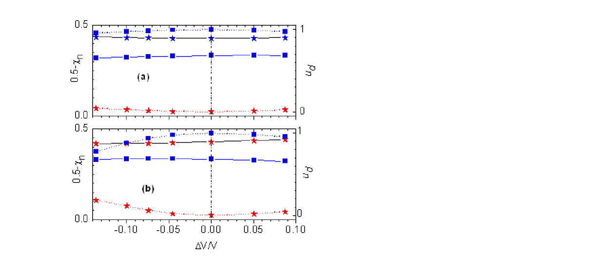
Figure 2: Changes of the two most relevant DFs (left side and continuous lines) and of their weights (right side and dotted lines) with respect to shape variation from sphere. The shape variation is accounted by the volume variation $\Delta V/V$. The first (dipole)/the second (octopole) eigenmode is denoted by the square/star symbol. The field polarization is (a) parallel or (b) perpendicular to the rotation axis.

Throughout this work I consider small shape variations of gold NPs immersed in water ($n_{water}$=1.33). The Drude parameters of gold are those that are usually used in the literature. Thus, in energy, the plasma frequency $\omega_{p}$ is about 9 eV and $\gamma$ is about 0.1 eV Sandu et al. (2011). Also the interband $\varepsilon_{m}$ is adjusted to have the LSPR for a nanosphere at 530 nm, i.e., $\varepsilon_{m}=10.2$. Fig. 2 illustrates the variations of the two most relevant eigenvalues (or equivalently the associated DFs) and their weights with respect to shape variation from a nanosphere and field polarization. An eigenmode is considered relevant if its weight may exceed 1%. The relative volume ${\Delta V}/V$ varies with respect to spherical shape from -14% to 10%. Fig. 3 presents the variation of LSPR spectra with respect to both shape variation and field polarization. The shape variations are hardly detected by simple vizualization as one can see from the inset of Fig 3b, which shows the variations in cross-section for volume variations up to 14%.

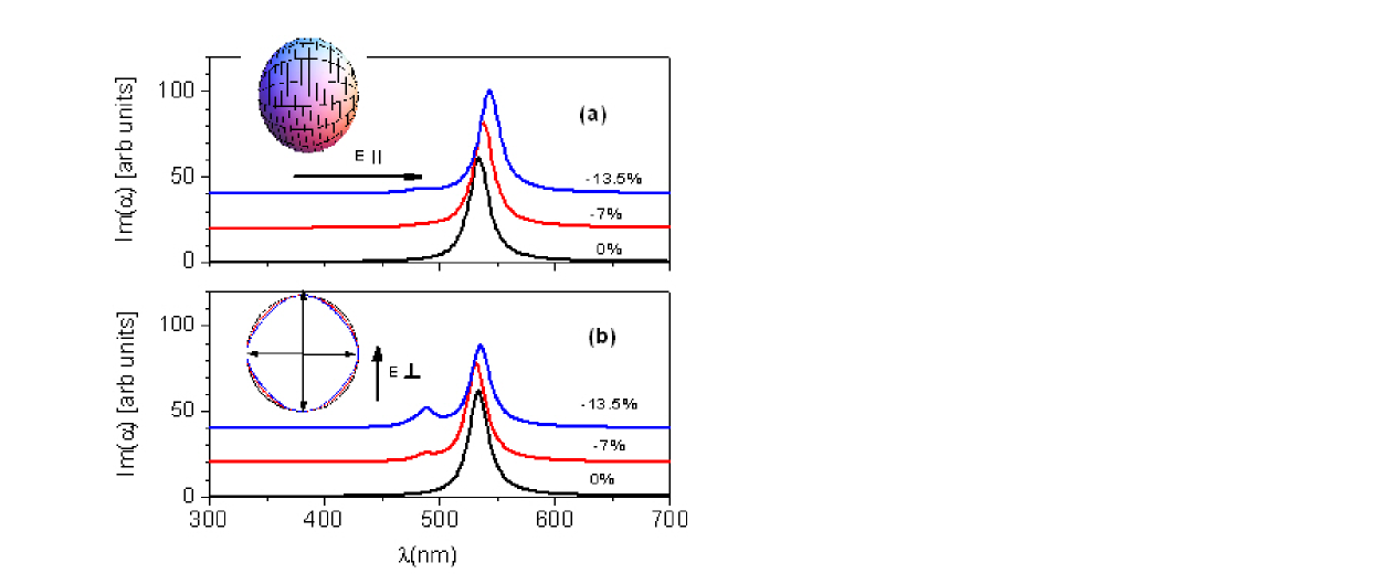
Figure 3: The LSPR spectra for three different $\Delta V/V$: -0%, -7%, and -13.5%. For a better visualization the spectra are moved upwards accordingly. The field polarization is (a) parallel or (b) perpendicular to the rotation axis. The inset of (a) depicts a sphere and the field polarizations. The inset of (b) represents the cross-section variations corresponding to shape variations.

For parallel polarization, the first relevant eigenmode represents the dipole response and has a monotonic ( i. e. increasing) behavior of its DF with respect to volume variation. Therefore, according to Eq. 7 a smaller DF means a redshifted LSPR as it is observed from Fig 2a and 3a at negative volume variations. The NP is invariant with respect to coordinate change $z\leftrightarrow-z$, thus the quadrupole eigenmode is not allowed to be bright, therefore the second most relevant eigenmode is the octopolar eigenmode. In contrast to the dipolar one, the octopolar eigenmode exhibits a non-monotonic variation of the DF with a minimum reached when the particle is spherical ($\Delta V/V=0$%). No major variation of its weight (i. e. no more than 10%), however, occurs with no noticeable change in the LSPR spectrum. Thus, from Fig 3a and according to the first sum rule $\sum\limits_{k}{p_{k}}=1$ (Sandu et al. 2010), the weight variation of the dipole eigenvalue is also less than 10%.

There is a different picture for transverse polarization (Fig. 2b and Fig 3b). The DF of the dipole eigenvalue is non-monotonic with a maximum around $\Delta V/V=-10$ % and its weight varies by -20% for a volume variation of -13.6%. Moreover, for positive $\Delta V/V$, the LSPR of the dipole eigenmode redshifts as a result of the DF drop. The large reduction of the dipolar weight is reflected in large increase of the octopolar weight, which can be also seen in the LSPR spectrum plotted in Fig 3b. At the same time the DF of the octopolar eigenmode increases with $\Delta V/V$.

III.3 Changes due to the variation from prolate shape

The changes of the electrostatic resonances due to smooth variation from a prolate shape are shown in Fig. 4, where only the two most relevant eigenvalues and their weights are presented. The aspect ratio is 2. For both field polarizations, ${\Delta V}/V$ varies over a wider range from -24% to 11%. The behavior of LSPR spectra with respect to shape variations can be seen in Fig. 5. The shape variations that are defined by volume variations can be vizualized in the left inset of Fig 5. Like in the previous case, the quadrupole eigenmode is dark, regardless of shape change. When the polarization is longitudinal, the DFs of the most relevant eigenmodes (dipolar and octopolar) vary smoothly over the entire range of volume variation considered here. The corresponding LSPRs can be noticed at longer wavelengths in Fig. 5. While the DF of the octopole eigenmode increases with ${\Delta V}/V$, the DF of the dipole eigenmode reaches its maximum at ${\Delta V}/V=-11\%$. The LSPRs are sensitive to shape variations, such that at ${\Delta V}/V=-11\%$, an octopolar bump can be seen in the spectrum. The bump transforms into a distinct LSPR at ${\Delta V}/V=-23\%$.

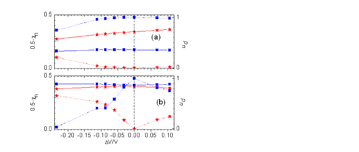
Figure 4: Changes of the two most relevant DFs (left side and continuous lines) and of their weights (right side and dotted lines) with respect to shape variation from prolate spheroidal shape. The shape variation is accounted by $\Delta V/V$. The first (dipolar)/second (octopolar) eigenmode is denoted by the square/star symbol. The field polarization is (a) parallel or (b) perpendicular to the rotation axis.

The behavior is however quite different for transverse polarization, where the cross-section is smaller. Dramatic changes in the weights of the relevant eigenmodes are found although the eigenvalues and their DFs vary smoothly. The appearance of the octopolar eigenmode in the LSPR spectrum occurs for a volume variation as small as $\pm 5\%$. The DF of the dipole eigenmode is non-monotonic with a minimum at $\Delta V/V=0$ and a maximum around $\Delta V/V=-11\%$. An interesting behavior occurs around $\Delta V/V=-10\%$, where the shape looks rather like an American football (Fig. 6a) and the weight of the octopolar eigenmode surpasses the weight of the dipolar eigenmode. The weight of the dipole eigenmode varies from 100% at $\Delta V/V=0$ to a value of around 40% for a volume variation of -11% (Fig 4b). Moreover, for small positive and negative $\Delta V/V$, the LSPR of the dipole eigenmode blueshifts as a result of the DF increase. The large reduction of the dipolar weight is reflected in large increase of the octopolar weight, which can be also seen in the LSPR spectrum plotted in Fig 5b. At the same time the DF of the octopolar eigenmode reaches its maximum at $\Delta V/V=-3\%$.

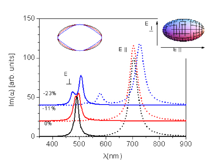
Figure 5: The LSPR spectra for three different $\Delta V/V$: 0%, -11%, and -23%. For a better visualization the spectra are moved upwards accordingly. The field polarization is parallel (dotted lines and the LSPRs at longer wavelengths) or perpendicular (solid lines and the LSPRs at shorter wavelenghts) to the rotation axis. The insets depict a prolate spheroid and the field polarizations (right side) and the axial cross-section variations corresponding to shape variations (left side).

To understand why the octopole weight exceeds the dipole weight it is better to inspect the dipole and the octopole eigenfunctions of $\hat{M}$ for both shapes: the spheroidal prolate shape and the football-like shape obtained by a volume variation of -11%. These eigenfunctions are plotted in Fig. 6. Due to the axial symmetry, for a transverse polarization, the eigenvectors have the following expression $u\left({z,\varphi}\right)=u_{1}\left(z\right)\sin\varphi$, when the field is along the y-axis. The functions $u_{1}\left(z\right)$ of both the dipole and the octopole eigenmodes are plotted in Fig. 5. Thus the dipole eigenmode represents a large dipole ($\uparrow)$ concentrated in the middle of the NP in the case of spheroidal shape (Fig. 6b) and splits into two parallel dipoles ($\uparrow\uparrow)$ towards the extremities for a football-like shape (Fig. 6a). These two parallel dipoles are much smaller than the spheroidal dipole because the extremities are much tighter than the middle of the NP. It is worth noticing that the dipolar character of the eigenmode is provided by the factor $\sin\varphi$ of the eigenfunction. At the same time, the octopole eigenmode has the dipole configuration $\downarrow\uparrow\downarrow$ but the total dipole moment vanishes for the spheroidal shape and it is different from 0 for the football shape. Also the dipolar contribution of the octopole eigenmode exceeds the contribution of the dipole eigenmode because the football-like NP is much thicker in the middle than toward the extremities.

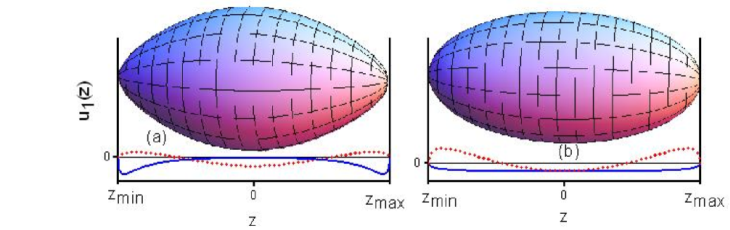
Figure 6: The z-dependent part u₁(z) of the dipole (solid line) and octopole (dotted line) eigenfunctions for (a) football-like and (b) prolate spheroidal NPs. For transverse polarization the full eigenfunctions have an extra factor $\sin\phi$. The shape of these NPs are depicted in the insets.

III.4 Changes due to the variation from oblate shape

The variations of the DFs and of their weights for the most relevant eigenvalues with respect to shape variation of an oblate spheroid and field polarization are presented in Fig. 7. The aspect ratio is taken to be 1/2. The axial polarization exhibits three relevant eigenmodes, while the transverse polarization has just two relevant eigenmodes. The variation of the relative volume ${\Delta V}/V$ spans between -14% and 14%. Fig. 8 shows the variation of LSPR spectra with respect to both shape variation and field polarization.

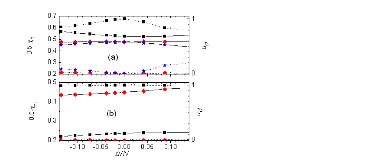
Figure 7: Changes of the relevant DFs (left side and continuous lines) and of their weights (right side and dotted lines) with respect to shape variation from oblate spheroidal shape. The first eigenmode (dipolar) is denoted by square symbol. The other eigenmodes are denoted by star and diamond symbols. The field polarization is (a) parallel or (b) perpendicular to the rotation axis.

The electric field parallel with the rotation axis is considered first. In this case the LSPRs are found at shorter wavelenghts in Fig. 8. The first relevant eigenmode represents also the dipole response and its corresponding DF has a non-monotonic behavior by having the minimum at ${\Delta V}/V=4\%$. Thus there is a blueshift of the corresponding LSPR for negative $\Delta V/V$ (see Fig. 8). The next most relevant is the octopole eigenmode which can be seen as a bump for a volume variation of -7.4% and a quite distinct new resonance at ${\Delta V}/V=-13.5\%$. The weight of the third relevant eigenmode does not exceed 2% over entire range of $\Delta V/V$, therefore this eigenmode is not seen in the LSPR spectrum. The variations of DFs of the octopole and the third relevant eigenmode are non-monotonic. The octopole eigenmode has a minimum at ${\Delta V}/V=0$ and a maximum around ${\Delta V}/V=-7.5\%$, while the third relevant eigenmode has a maximum at ${\Delta V}/V=0$. For transverse polarization the modifications of the DFs of the two most relevant eigenmodes (the dipole and the octopole) increase with $\Delta V/V$ such that for negative/positive $\Delta V/V$ there is a redshift/blueshift of the dipole LSPR. The calculations also show that the octopole eigenmode does not show up in the LSPR spectrum.

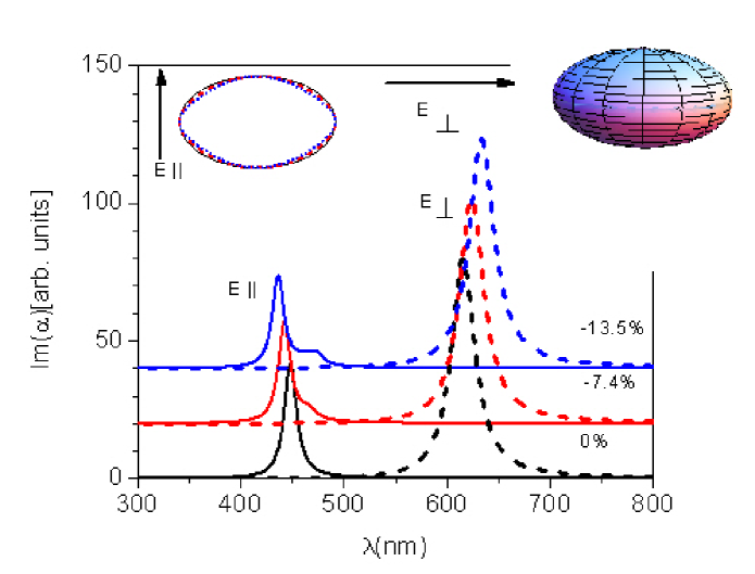
Figure 8: The LSPR spectra for three different $\Delta V/V$: 0%, -7.4%, and -13.5%. For a better visualization the spectra are moved upwards accordingly. The field polarization is parallel (full line and the LSPRs at shorter wavelengths) or perpendicular (dotted line and the LSPRs at longer wavelenghts) to the rotation axis. The inset depicts an oblate spheroid (right side) and the axial cross-section variations corresponding to volume variations (left side).

IV Conclusions

In the quasistatic approximation I use a BIE method to analyze the changes of LSPRs produced by small and smooth variations of the shape of metallic NPs. The LSPRs are determined by the eigenvalues and their coupling weights that come from the operator associated to the BIE method. First, the numerical implementation of BIE is verified against well known results. Thus for axially symmetric structures the method has an excellent accuracy. Also a compact formula of the NP polarizability is used to elaborate a criterion for the structural changes of the spectrum with respect to shape variation. Such shape variations are inherent to NP fabrication process. Shape variations induce changes in both the eigenvalues and their coupling weights to the electromagnetic field. However, the coupling weights appear to be more affected by shape changes, such that they manifest as structural modifications of the LSPR spectrum. Full numerical calculations show that structural modifications of the optical response occur for shape changes corresponding to volume variations greater than 12%. This quantitative result can be directly related to the criterion provided by Eq. (11), where a variation of $p_{k}>0.1$ would generate structural changes in LSPR spectrum. A 0.1 variation of $p_{k}$ means a 10% volume variation via the definition of $p_{k}$, which is inverse proportional to volume $V$. Therefore the NP volume variation contributes significantly to the structural changes of the LSPR spectrum which is agreement to other results regarding the averaging effect of the roughness on the LSPRs of metallic NPs Trugler et al. (2011). The largest optical changes are encountered for light polarization that is parallel to the smallest cross-sections of NPs. This aspect is important because more care must be considered for the design and the fabrication of the smallest features of the NP systems.