A simple and accurate approximation for the $Q$ stability parameter in multi-component and realistically thick discs

Abstract

In this paper, we propose a $Q$ stability parameter that is more realistic than those commonly used, and is easy to evaluate [see Eq. (19)]. Using our $\mathcal{Q}_{N}$ parameter, you can take into account several stellar and/or gaseous components as well as the stabilizing effect of disc thickness, you can predict which component dominates the local stability level, and you can do all that simply and accurately. To illustrate the strength of $\mathcal{Q}_{N}$, we analyse the stability of a large sample of spirals from The H i Nearby Galaxy Survey (THINGS), treating stars, H i and $\mathrm{H}_{2}$ as three distinct components. Our analysis shows that $\mathrm{H}_{2}$ plays a significant role in disc (in)stability even at distances as large as half the optical radius. This is an important aspect of the problem, which was missed by previous (two-component) analyses of THINGS spirals. We also show that H i plays a negligible role up to the edge of the optical disc; and that the stability level of THINGS spirals is, on average, remarkably flat and well above unity.

1 INTRODUCTION

Today, several decades after the pioneering work of Lin & Shu (1966) and the seminal papers by Jog & Solomon (1984a, b), it is widely accepted that stars and cold interstellar gas have an important interplay in the gravitational instability of galactic discs. The gravitational coupling between stars and gas does not alter the form of the local axisymmetric stability criterion, $Q\geq 1$ (Toomre 1964), but makes the $Q$ stability parameter dependent on the radial velocity dispersions and surface mass densities of the two components (Bertin & Romeo 1988; Elmegreen 1995; Jog 1996; Rafikov 2001; Shen & Lou 2003). The value of $Q$ is also affected by other factors, such as the vertical structure of the disc (Shu 1968; Romeo 1990, 1992, 1994; Elmegreen 2011; Romeo & Wiegert 2011), gas turbulence (Hoffmann & Romeo 2012; Shadmehri & Khajenabi 2012), and gas dissipation (Elmegreen 2011). Comprehensive analyses have shown that the two-component $Q$ parameter has a large impact on the dynamics and evolution of spiral structure in galaxies (see Bertin & Lin 1996), and is also a useful diagnostic for exploring the link between disc instability and star formation (Leroy et al. 2008).

Romeo & Wiegert (2011) introduced a simple and accurate approximation for the two-component $Q$ parameter, which takes into account the stabilizing effect of disc thickness and predicts whether the local stability level is dominated by stars or gas. The Romeo-Wiegert approximation has been used for investigating the evolution of gravitationally unstable discs (Cacciato et al. 2012; Forbes et al. 2012), the spiral structure of NGC 5247 (Khoperskov et al. 2012), the dynamical link between dark matter and H i in nearby galaxies (Meurer et al. 2013), as well as the link between disc stability and the relative distributions of stars, gas and star formation (Zheng et al. 2013). Forbes et al. (2012) concluded that the Romeo-Wiegert approximation is much faster to use than the $Q$ stability parameter of Rafikov (2001): it speeds up their disc-evolution code by as much as one or two orders of magnitude! This is simply because such an approximation estimates $Q$ analytically, without the need to minimize the dispersion relation over all wavenumbers, as is usually done.

A fundamental problem that must be faced when analysing the stability of galactic discs is how to represent their complex structure using only two components. The results of such analyses are indeed very sensitive to the choice of the gaseous 1D velocity dispersion, $\sigma_{\mathrm{g}}$: the colder the gas, the stronger its impact on the stability of the disc (e.g., Jog & Solomon 1984a; Bertin & Romeo 1988). Choosing $\sigma_{\mathrm{g}}\approx 6\;\mbox{km\,s}^{-1}$ will represent molecular gas well (Wilson et al. 2011), but will overestimate the contribution of atomic gas and make the disc more unstable than it actually is. Vice versa, choosing $\sigma_{\mathrm{g}}\approx 11\;\mbox{km\,s}^{-1}$ will represent H i well (Leroy et al. 2008), but will underestimate the contribution of $\mathrm{H}_{2}$ and stabilize the disc artificially. Intermediate values or more elaborate choices of $\sigma_{\mathrm{g}}$ will still not solve the problem. This motivates the use of a proper multi-component $Q$ parameter.

One of the first papers that discussed the gravitational instability of multi-component discs dates back to Morozov (1981). This author derived a dispersion relation that is valid for infinitesimally thin discs made of gas and $N_{\star}$ stellar components. He also calculated the stability criterion for $N_{\star}=2$. Rafikov (2001) derived a stability criterion that is valid for any $N_{\star}$ and can easily be expressed in the usual form $Q\geq 1$.

In this paper, we introduce a new $Q$ stability parameter, which has the same strong advantages as the Romeo-Wiegert approximation, and which is applicable to fully multi-component and realistically thick discs [see Eq. (19)]. We also show how to use our $\mathcal{Q}_{N}$ parameter for analysing the stability of galactic discs, and illustrate the strength of a multi-component analysis. We do so using a large sample of spirals from The H i Nearby Galaxy Survey (THINGS), and treating stars, H i and $\mathrm{H}_{2}$ as three distinct components.

The rest of the paper is organized as follows. In Sect. 2, we review the basic case of two-component discs and further motivate the need for a multi-component analysis (Sect. 2.1), we present our $\mathcal{Q}_{N}$ parameter (Sects 2.2–2.4), and we analyse the stability of THINGS spirals (Sect. 2.5). In Sect. 3, we discuss the weaknesses of $\mathcal{Q}_{N}$, which are common to all $Q$ parameters and stability criteria quoted here. In Sect. 4, we draw the conclusions.

2 STAR-GAS INSTABILITIES AND THE $Q$ DIAGNOSTIC

2.1 Two components … or more? More!

Let us first discuss the case of two-component and infinitesimally thin discs, which is fundamental to a proper understanding of Sects 2.2–2.5. It is well known that the stability properties of such discs are determined by five basic quantities: the epicyclic frequency, $\kappa$, the stellar and gaseous surface densities, $\Sigma_{\star}$ and $\Sigma_{\mathrm{g}}$, the stellar radial velocity dispersion, $\sigma_{R\star}$, and the gaseous 1D velocity dispersion, $\sigma_{\mathrm{1D\,g}}$ (e.g., Lin & Shu 1966; Rafikov 2001). The last two quantities reflect an important dynamical difference between stars and cold interstellar gas. The stellar component is collisionless so its velocity dispersion is anisotropic, while gas is collisional and has an isotropic velocity dispersion (see, e.g., Binney & Tremaine 2008). Hereafter we will simplify the notation and denote the relevant velocity dispersions of the two components with $\sigma_{\star}$ and $\sigma_{\mathrm{g}}$.

Lin & Shu (1966) and Rafikov (2001) took those facts into account by treating stars as a kinetic component and gas as a fluid (see also Shu 1968). The resulting local axisymmetric stability criteria are equivalent because they are based on the same dispersion relation, $\omega^{2}(k)$, and because they are derived by imposing that $\omega^{2}(k)\geq 0$ for all $k$. However, Rafikov’s stability criterion is simpler and more used (e.g., Dalcanton et al. 2004; Li et al. 2005, 2006; Kim & Ostriker 2007; Yang et al. 2007; Yim et al. 2011). Such a criterion can be written as $Q_{\mathrm{Rk}}\geq 1$, where

$$\frac{1}{Q_{\mathrm{Rk}}}=\max\{\mathrm{SC}_{\mathrm{Rk}}(K)\}\,,$$ (1)

$$\mathrm{SC}_{\mathrm{Rk}}(K)=\frac{1}{Q_{\star}}\,\frac{2\left[1-\mathrm{e}^{-K^{2}}I_{0}\left(K^{2}\right)\right]}{K}+\frac{1}{Q_{\mathrm{g}}}\,\frac{2Ks}{1+K^{2}s^{2}}\,,$$ (2)

$$K=k\,\frac{\sigma_{\star}}{\kappa}\,,$$ (3)

$$Q_{\star}=\frac{\kappa\sigma_{\star}}{\pi G\Sigma_{\star}}\,,\;\;\;\;\;Q_{\mathrm{g}}=\frac{\kappa\sigma_{\mathrm{g}}}{\pi G\Sigma_{\mathrm{g}}}\,,$$ (4)

$$s=\frac{\sigma_{\mathrm{g}}}{\sigma_{\star}}\,.$$ (5)

In these equations, $Q_{\mathrm{Rk}}$ is Rafikov’s kinetic-fluid $Q$ parameter, $\mathrm{SC}_{\mathrm{Rk}}(K)$ is the related stability curve, $K$ is the radial wavenumber of the perturbation expressed in dimensionless form, $Q_{\star}$ and $Q_{\mathrm{g}}$ are the stellar and gaseous Toomre parameters, and $I_{0}$ denotes the modified Bessel function of the first kind and order zero.

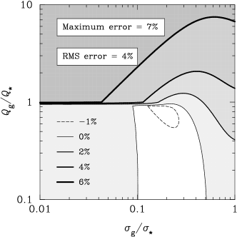
Figure 1: Accuracy of the two-fluid stability criterion. The curves shown are the contour lines of the relative error $(Q_{\mathrm{Rf}}-Q_{\mathrm{Rk}})/Q_{\mathrm{Rk}}$, where $Q_{\mathrm{Rf}}$ and $Q_{\mathrm{Rk}}$ are the fluid-fluid and kinetic-fluid $Q$ parameters of Rafikov (2001). In addition, $Q_{\star}$ and $Q_{\mathrm{g}}$ are the stellar and gaseous Toomre parameters, $\sigma_{\star}$ and $\sigma_{\mathrm{g}}$ are the relevant velocity dispersions of the two components.

Bertin & Romeo (1988), Elmegreen (1995), Jog (1996), and again Rafikov (2001) adopted a less rigorous, but more straightforward approach: they treated the stellar component as a fluid, with sound speed equal to $\sigma_{\star}$. The resulting two-fluid stability criteria are equivalent, apart from the different parametrizations used, because they are based on the same dispersion relation (Jog & Solomon 1984a). However, even in this case, Rafikov’s criterion is simpler and is becoming more and more widely used (e.g., Leroy et al. 2008; Robertson & Kravtsov 2008; Dekel et al. 2009; Mastropietro et al. 2009; Ceverino et al. 2010; Westfall et al. 2011; Elson et al. 2012; Watson et al. 2012; Williamson & Thacker 2012). Such a criterion can be written as $Q_{\mathrm{Rf}}\geq 1$, where Rafikov’s fluid-fluid $Q$ parameter can be computed by maximizing the related stability curve over all radial wavenumbers:

$$\frac{1}{Q_{\mathrm{Rf}}}=\max\{\mathrm{SC}_{\mathrm{Rf}}(K)\}\,,$$ (6)

$$\mathrm{SC}_{\mathrm{Rf}}(K)=\frac{1}{Q_{\star}}\,\frac{2K}{1+K^{2}}+\frac{1}{Q_{\mathrm{g}}}\,\frac{2Ks}{1+K^{2}s^{2}}\,.$$ (7)

What is the accuracy of the two-fluid stability criterion? Bertin & Romeo (1988) compared the fluid-fluid and kinetic-fluid marginal stability curves in a representative set of cases, and showed that the differences are small (see their fig. 2). Rafikov (2001) carried out a more detailed analysis and got similar results (see his fig. 3). However, he did not evaluate the relative error $(Q_{\mathrm{Rf}}-Q_{\mathrm{Rk}})/Q_{\mathrm{Rk}}$, which depends on $s$ and

$$q=\frac{Q_{\mathrm{g}}}{Q_{\star}}\,,$$ (8)

and which is a useful piece of information for assessing the accuracy of $Q_{\mathrm{Rf}}$. We do this in Fig. 1. Our contour map shows that such error is less than 7% and has a root-mean-square value of 4%. This means that $Q_{\mathrm{Rf}}$ and $Q_{\mathrm{Rk}}$ are practically equivalent, since the parameters $s$ and $q$ are themselves subject to observational uncertainties.

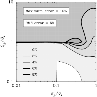
Figure 2: Accuracy of the Romeo-Wiegert approximation. The curves shown are the contour lines of the relative error $(Q_{\mathrm{RW}}-Q_{\mathrm{Rk}})/Q_{\mathrm{Rk}}$, where $Q_{\mathrm{RW}}$ is the two-component $Q$ parameter of Romeo & Wiegert (2011), and $Q_{\mathrm{Rk}}$ is the kinetic-fluid $Q$ parameter of Rafikov (2001). The rest of the notation is the same as in Fig. 1.

Romeo & Wiegert (2011) showed that the two-fluid $Q$ parameter can be accurately estimated without the usual maximization (or minimization) procedure:

$$\frac{1}{Q_{\mathrm{RW}}}=\left\{\begin{array}[]{ll}{\displaystyle\frac{W}{Q_{\star}}+\frac{1}{Q_{\mathrm{g}}}}&\mbox{if\ }Q_{\star}\geq Q_{\mathrm{g}}\,,\\ &\\ {\displaystyle\frac{1}{Q_{\star}}+\frac{W}{Q_{\mathrm{g}}}}&\mbox{if\ }Q_{\mathrm{g}}\geq Q_{\star}\,;\end{array}\right.$$ (9)

$$W=\frac{2\sigma_{\star}\sigma_{\mathrm{g}}}{\sigma_{\star}^{2}+\sigma_{\mathrm{g}}^{2}}\,.$$ (10)

Although very recent, such an approximation is already frequently used (e.g., Cacciato et al. 2012; Forbes et al. 2012; Hoffmann & Romeo 2012; Khoperskov et al. 2012; Meurer et al. 2013; Zheng et al. 2013). Fig. 2 shows that $Q_{\mathrm{RW}}$ is remarkably accurate even with respect to the kinetic-fluid $Q$ parameter. In fact, the relative error $(Q_{\mathrm{RW}}-Q_{\mathrm{Rk}})/Q_{\mathrm{Rk}}$ is below 10% and has a root-mean-square value of 5%. Thus $Q_{\mathrm{RW}}$ is a faster and physically equivalent alternative to $Q_{\mathrm{Rf}}$ or $Q_{\mathrm{Rk}}$.

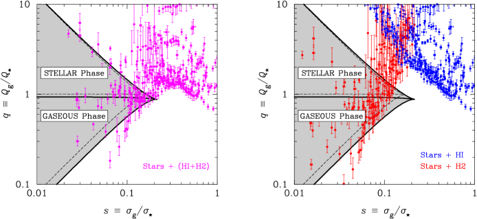
Figure 3: Why a multi-component analysis is needed: the parameter plane of star-gas instabilities populated by THINGS spirals. The cases illustrated in the two panels are stars plus gas (left), and stars plus H i or $\mathrm{H}_{2}$ (right). The galaxy data are from Leroy et al. (2008), $Q_{\star}$ and $Q_{\mathrm{g}}$ are the stellar and gaseous Toomre parameters, $\sigma_{\star}$ and $\sigma_{\mathrm{g}}$ are the relevant velocity dispersions of the two components. The shaded part of the $(s,q)$ plane represents the condition for star-gas decoupling, with the stellar component treated as collisionless (thick solid lines) or collisional (thin dashed lines). This is the ‘two-phase region’ discussed in the text. The boundaries of this region and the transition line intersect at $(s,q)\simeq(0.21,0.88)$ in the collisionless case, and at $(s,q)\simeq(0.17,1)$ in the collisional case.

To understand the weaknesses of a two-component analysis, let us see how spiral galaxies populate the parameter plane of star-gas instabilities. We use a sample of twelve nearby star-forming spirals from THINGS, previously analysed by Leroy et al. (2008) and Romeo & Wiegert (2011): NGC 628, 2841, 3184, 3198, 3351, 3521, 3627, 4736, 5055, 5194, 6946 and 7331. For each galaxy of this sample, we compute the radial profiles $s=s(R)$ and $q=q(R)$, and hence the track left by the galaxy in the $(s,q)$ plane. The result for the whole sample is shown in the left panel of Fig. 3. Note that 20% of the data fall within the shaded part of the $(s,q)$ plane, which represents the condition for star-gas decoupling. In this region, $\mathrm{SC}_{\mathrm{Rk}}(K)$ has two maxima: one at small $K$, where the response of the stellar component peaks; and the other at large $K$, where gas dominates. In the ‘stellar phase’, the maximum at small $K$ is higher than the other one, and therefore it controls the onset of disc instability. Vice versa, in the ‘gaseous phase’, it is the maximum at large $K$ that determines $Q_{\mathrm{Rk}}$. The two-fluid counterpart of this region (thin dashed lines) is also populated by 20% of the data (Romeo & Wiegert 2011). In the rest of the parameter plane, the dynamical responses of the two components are strongly coupled and peak at a single wavelength.

The analysis of THINGS spirals carried out above treats the interstellar medium (ISM) as a single component with $\Sigma_{\mathrm{g}}=\Sigma_{\mathrm{HI}}+\Sigma_{\mathrm{H2}}$ and $\sigma_{\mathrm{g}}=11\;\mbox{km\,s}^{-1}$ (Leroy et al. 2008). What are the limitations of this approach? How do H i and $\mathrm{H}_{2}$ contribute to star-gas instabilities? To answer these questions, we consider H i and $\mathrm{H}_{2}$ separately, and choose observationally motivated values of the 1D velocity dispersion: $\sigma_{\mathrm{HI}}=11\;\mbox{km\,s}^{-1}$ (Leroy et al. 2008), and $\sigma_{\mathrm{H2}}=6\;\mbox{km\,s}^{-1}$ (Wilson et al. 2011). We then compute the $(s,q)$ tracks for each case (stars plus H i or $\mathrm{H}_{2}$), and show the results in the right panel of Fig. 3. Note that H i and $\mathrm{H}_{2}$ populate the parameter plane differently. In particular, none of the H i data falls within the two-phase region, while $\mathrm{H}_{2}$ populates such a region in 60% of the cases. This means that H i and $\mathrm{H}_{2}$ have distinct stability properties, and a fundamentally different dynamical coupling with stars. Treating the ISM as a single component underestimates the role that $\mathrm{H}_{2}$ plays in star-gas instabilities, and overestimates the contribution of H i. This is why a multi-component analysis is needed!

2.2 Approximating $Q$ in the thin-disc limit

The only multi-component stability diagnostics that have been available so far are the local axisymmetric stability criteria of Morozov (1981) and Rafikov (2001), which are valid for infinitesimally thin discs made of gas and $N_{\star}$ stellar components. For $N_{\star}=2$, the case considered by Morozov (1981), such criteria are equivalent because they are based on similar approximations. However, besides being more general, Rafikov’s criterion is simpler and can be written as $Q_{\mathrm{R},N}\geq 1$, where

$$\frac{1}{Q_{\mathrm{R},N}}=\max\{\mathrm{SC}_{\mathrm{R},N}(k)\}\,,$$ (11)

$$\mathrm{SC}_{\mathrm{R},N}(k)=\frac{1}{Q_{1}}\,\frac{2K_{1}}{1+K_{1}^{2}}+\sum_{i=2}^{N}\frac{1}{Q_{i}}\,\frac{2\left[1-\mathrm{e}^{-K_{i}^{2}}I_{0}\left(K_{i}^{2}\right)\right]}{K_{i}}\,,$$ (12)

$$K_{i}=k\,\frac{\sigma_{i}}{\kappa}\,,$$ (13)

$$Q_{i}=\frac{\kappa\sigma_{i}}{\pi G\Sigma_{i}}\,.$$ (14)

Let us illustrate how to find a simple, accurate, fast and more general $Q$ diagnostic. In Sect. 2.1, we have shown that stars can be accurately treated as a fluid when evaluating $Q$. So we can safely replace the kinetic terms in Eq. (12) with their fluid counterparts. We then face the heart of the problem: how to estimate the least stable wavenumber, $k_{\mathrm{max}}$, without the usual maximization procedure. Consider the two-component case first, and compare the Romeo-Wiegert approximation [Eqs (9) and (10)] with the two-fluid stability parameter [Eqs (6) and (7)]. One can easily infer that $K_{\mathrm{max}}$ fulfils the following conditions:

1. If $Q_{\star}>Q_{\mathrm{g}}$, then $2K_{\mathrm{max}}/(1+K_{\mathrm{max}}^{2})\sim W$ and $2K_{\mathrm{max}}s/(1+K_{\mathrm{max}}^{2}s^{2})\sim 1$. As $W=2s/(1+s^{2})$, this implies that $K_{\mathrm{max}}\sim 1/s$, i.e. $k_{\mathrm{max}}\sim\kappa/\sigma_{\mathrm{g}}$.

2. If $Q_{\mathrm{g}}>Q_{\star}$, then $2K_{\mathrm{max}}/(1+K_{\mathrm{max}}^{2})\sim 1$ and $2K_{\mathrm{max}}s/(1+K_{\mathrm{max}}^{2}s^{2})\sim W$. This implies that $K_{\mathrm{max}}\sim 1$, i.e. $k_{\mathrm{max}}\sim\kappa/\sigma_{\star}$.

Conditions (i) and (ii) have not been pointed out in previous analyses. They simply mean that $1/k_{\mathrm{max}}$ is approximately the typical epicycle size of the less stable component. This approximation is not accurate when $s\approx 0.2$ and $q\approx 1$, since for such values there is a transition between three stability regimes and $K_{\mathrm{max}}$ has a jump across one of the interfaces (see discussion of Fig. 3). Note, however, that estimating $K_{\mathrm{max}}$ as above produces a very accurate estimate of $Q_{\mathrm{Rf}}$, namely the Romeo-Wiegert approximation. This is because $Q_{\mathrm{Rf}}$ is continuous across the $q=1$ line, and because the error that affects the estimate of $Q_{\mathrm{Rf}}$ is of second order with respect to that of $K_{\mathrm{max}}$: $\Delta Q_{\mathrm{Rf}}\propto(\Delta K_{\mathrm{max}})^{2}$. The first-order term is obviously zero, since the first derivative of $\mathrm{SC}_{\mathrm{Rf}}(K)$ vanishes for $K=K_{\mathrm{max}}$. This flow of arguments suggests that we can estimate the $N$-component $Q$ parameter as in the two-fluid case, i.e. by approximating $1/k_{\mathrm{max}}$ with the typical epicycle size of the least stable component ($k_{\mathrm{max}}\sim\kappa/\sigma_{m}$):

$$\frac{1}{Q_{N}}=\sum_{i=1}^{N}\frac{W_{i}}{Q_{i}}\,,$$ (15)

$$W_{i}=\frac{2\sigma_{m}\sigma_{i}}{\sigma_{m}^{2}+\sigma_{i}^{2}}\,,$$ (16)

where the index $m$ denotes the component with smallest $Q$: $Q_{m}=\min\{Q_{i}\}$. This is the component that dominates the local stability level ($W_{m}=1$). All other components have less weight; the more $\sigma_{i}$ differs from $\sigma_{m}$, the smaller the weight factor $W_{i}$.

What is the accuracy of $Q_{N}$? In Appendix A, we show how estimation uncertainties propagate from $W_{i}$ to $Q_{N}$, and derive an upper bound for the resulting root-mean-square error:

$$\frac{\Delta Q_{N}}{Q_{N}}\la 0.03\,\sqrt{N}\,.$$ (17)

Eq. (17) tells us that the accuracy of our approximation deteriorates slowly as we consider more and more components. In the case of greatest interest, stars plus H i plus $\mathrm{H}_{2}$, the relative error is on average less than 6%, i.e. almost as low as in the two-component case (see Fig. 2).

Table 1: Accuracy of our approximation in the ten-component cases analysed by Rafikov (2001).

Case	$Q_{\mathrm{R},N}$	$Q_{N}$	$(Q_{N}-Q_{\mathrm{R},N})/Q_{\mathrm{R},N}$
1	1.10	1.12	1.8%
2	1.00	1.04	3.7%
3	1.00	1.04	4.5%
4	1.00	1.01	0.8%
4+1	1.00	1.01	1.2%

$Q_{\mathrm{R},N}$ is the $N$-component $Q$ parameter of Rafikov (2001), $Q_{N}$ is our $N$-component $Q$ parameter, and $(Q_{N}-Q_{\mathrm{R},N})/Q_{\mathrm{R},N}$ is the relative error of our approximation.

To demonstrate the accuracy of our approximation, we put it to a stringent test: the 10-component model of the Solar neighbourhood analysed by Rafikov (2001). That model includes cold interstellar gas, giants, stars in six luminosity ranges, white and brown dwarfs. Rafikov also analysed the effect of varying the most uncertain model parameters. He motivated and discussed five cases, which we summarize in Appendix B. For each case, we compare $Q_{N}$ with Rafikov’s $Q_{\mathrm{R},N}$ parameter and compute the relative error $(Q_{N}-Q_{\mathrm{R},N})/Q_{\mathrm{R},N}$. Table 1 shows that our approximation is remarkably accurate. In all cases, the relative error is less than 5%, which means twice as low as the upper bound predicted by Eq. (17).

2.3 Adding the effect of disc thickness

Our approximation is not yet complete. It does not include the stabilizing effect of disc thickness, which is important and should be taken into account when analysing the stability of galactic discs (Romeo & Wiegert 2011). In this section, we generalize the Romeo-Wiegert approach and provide a simple recipe for adding such an effect.

From the thin-disc limit, we have learned that the local stability level is dominated by the component with smallest $Q$ [see Eqs (15) and (16)]. The contributions of the other components are weakened by the $W_{i}$ factors, which are different and small if the components are dynamically distinct. In this case, we can estimate the effect of thickness reasonably well by considering each component separately. Romeo (1994) analysed this case in detail. The effect of thickness is to increase the stability parameter of each component by a factor $T$, which depends on the ratio of vertical to radial velocity dispersion:

$$T\approx\left\{\begin{array}[]{ll}{\displaystyle 1+0.6\left(\frac{\sigma_{z}}{\sigma_{R}}\right)^{2}}&\mbox{for\ }0\la\sigma_{z}/\sigma_{R}\la 0.5\,,\\ &\\ {\displaystyle 0.8+0.7\left(\frac{\sigma_{z}}{\sigma_{R}}\right)}&\mbox{for\ }0.5\la\sigma_{z}/\sigma_{R}\la 1\,.\end{array}\right.$$ (18)

Eq. (18) can be inferred from fig. 3 (top) of Romeo (1994). The range $0\la\sigma_{z}/\sigma_{R}\la 0.5$ is characteristic of the old stellar disc in Sc–Sd galaxies (Gerssen & Shapiro Griffin 2012), while $0.5\la\sigma_{z}/\sigma_{R}\la 1$ is the usual range of velocity anisotropy (typical of the old stellar disc in Sa–Sbc galaxies, of young stars and the ISM). To approximate $Q$ in this more general context, use then Eq. (15) with $Q_{i}$ replaced by $T_{i}Q_{i}$:

$$\frac{1}{\mathcal{Q}_{N}}=\sum_{i=1}^{N}\frac{W_{i}}{T_{i}Q_{i}}\,,$$ (19)

where $\mathcal{Q}_{N}$ is our $Q$ stability parameter for multi-component and realistically thick discs, $Q_{i}=\kappa\sigma_{i}/\pi G\Sigma_{i}$ is the Toomre parameter of component $i$, $T_{i}$ is given by Eq. (18), and $W_{i}$ is given by Eq. (16). NOTE that the index $m$ now denotes the component with smallest $TQ$: $T_{m}Q_{m}=\min\{T_{i}Q_{i}\}$. This is the component that dominates the local stability level. The contributions of the other components are still suppressed by the $W_{i}$ factors.

2.4 What about the effect of ISM turbulence?

Turbulence plays a fundamental role in the dynamics and structure of cold interstellar gas (see, e.g., Elmegreen & Scalo 2004; McKee & Ostriker 2007; Agertz et al. 2009). The most basic aspect of interstellar turbulence is the presence of supersonic motions. These are usually taken into account by identifying $\sigma_{\mathrm{g}}$ with the typical 1D velocity dispersion of the medium, rather than with its thermal sound speed. Another important aspect of interstellar turbulence is the existence of scaling relations between $\Sigma_{\mathrm{g}}$, $\sigma_{\mathrm{g}}$ and the size of the region over which such quantities are measured ($\ell$). Observations show that $\Sigma_{\mathrm{HI}}\sim\ell^{1/3}$ and $\sigma_{\mathrm{HI}}\sim\ell^{1/3}$ up to scales of 1–10 kpc, whereas $\Sigma_{\mathrm{H2}}\sim constant$ and $\sigma_{\mathrm{H2}}\sim\ell^{1/2}$ up to scales of about 100 pc (see, e.g., Elmegreen & Scalo 2004; McKee & Ostriker 2007; Romeo et al. 2010).

Motivated by the large observational uncertainties of $\Sigma_{\mathrm{g}}(\ell)$ and $\sigma_{\mathrm{g}}(\ell)$, and having in mind near-future applications to high-redshift galaxies, Romeo et al. (2010) considered more general scaling relations, $\Sigma_{\mathrm{g}}\propto\ell^{a}$ and $\sigma_{\mathrm{g}}\propto\ell^{b}$, and explored the effect of turbulence on the gravitational instability of gas discs. They showed that turbulence excites a rich variety of stability regimes, several of which have no classical counterpart. See in particular the ‘stability map of turbulence’ (fig. 1 of Romeo et al. 2010), which illustrates such stability regimes and populates them with observations, simulations and models of ISM turbulence. Hoffmann & Romeo (2012) extended this investigation to two-component discs of stars and gas, and analysed the stability of THINGS spirals. They showed that ISM turbulence alters the condition for star-gas decoupling and increases the least stable wavelength, but hardly modifies the $Q$ parameter at scales larger than about 100 pc. Since these are the usual scales of interest, we do not include that effect in our approximation.

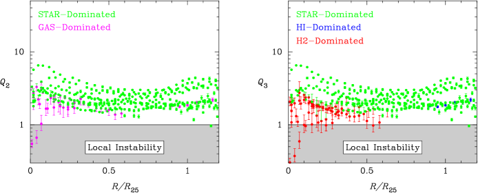
Figure 4: The stability level of THINGS spirals. The diagnostics used in the left and right panels are our $\mathcal{Q}_{2}$ and $\mathcal{Q}_{3}$ parameters [see Eq. (19) for $N=2,3$]. The galaxy data are from Leroy et al. (2008), $R$ is the galactocentric distance, and $R_{25}$ is the optical radius. The data are colour-coded so as to show whether the stability level is dominated by stars or gas (H i/$\mathrm{H}_{2}$), as predicted by Eq. (19). In the right panel, the three data points that lie well below the critical stability level tell us that the nuclear region of NGC 6946 is subject to strong $\mathrm{H}_{2}$-dominated instabilities. This is consistent with the facts that NGC 6946 hosts a nuclear starburst (e.g., Engelbracht et al. 1996) and a nuclear ‘bar within bar’ (e.g., Fathi et al. 2007).

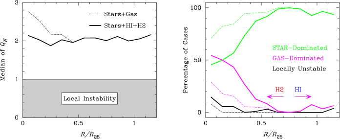
Figure 5: Stability characteristics of THINGS spirals. The radial profiles shown in the left and right panels are computed by binning the $\mathcal{Q}_{N}$ data of Fig. 4 in 12 rings of width $0.1\,R/R_{25}$, where $\mathcal{Q}_{N}$ is our $Q$ stability parameter for multi-component and realistically thick discs [see Eq. (19) for $N=2,3$], $R$ is the galactocentric distance, and $R_{25}$ is the optical radius. The right panel shows how frequently the stability level is dominated by stars or gas (H i/$\mathrm{H}_{2}$), and how frequently $\mathcal{Q}_{N}<1$. The thick solid lines are the predictions of a three-component analysis (stars plus H i plus $\mathrm{H}_{2}$), while the thin dashed lines represent the two-component case (stars plus gas).

2.5 Application to THINGS spirals

Our approximation is now complete. Let us then show how to use our $\mathcal{Q}_{N}$ parameter for analysing the stability of galactic discs, and illustrate the strength of a multi-component analysis.

In the following, we generalize the two-component approach of Romeo & Wiegert (2011). We consider the same sample of spiral galaxies as in Sect. 2.1 and refer to Leroy et al. (2008), hereafter L08, for a detailed description of the data and their translation into physical quantities. We treat stars, H i and $\mathrm{H}_{2}$ as three components with the same surface densities and $\sigma_{\star}$ as in L08, but with distinct values of $\sigma_{\mathrm{g}}$: $\sigma_{\mathrm{HI}}=11\;\mbox{km\,s}^{-1}$ (L08), and $\sigma_{\mathrm{H2}}=6\;\mbox{km\,s}^{-1}$ (Wilson et al. 2011). For each galaxy, we compute the radial profile of $\mathcal{Q}_{3}$ using Eq. (19). We adopt $(\sigma_{z}/\sigma_{R})_{\star}=0.6$, as was assumed by L08, and $(\sigma_{z}/\sigma_{R})_{\mathrm{HI}}=(\sigma_{z}/\sigma_{R})_{\mathrm{H2}}=1$, as is natural for collisional components. For comparison purposes, we also compute the radial profile of $\mathcal{Q}_{2}$, treating the ISM as a single component with $\Sigma_{\mathrm{g}}=\Sigma_{\mathrm{HI}}+\Sigma_{\mathrm{H2}}$ and $\sigma_{\mathrm{g}}=11\;\mbox{km\,s}^{-1}$ (L08).

Fig. 4 shows $\mathcal{Q}_{3}(R)$ and $\mathcal{Q}_{2}(R)$ for the whole galaxy sample. Note that the $\mathcal{Q}_{3}$ data are characterized by a sharp transition at about half the optical radius. For $R\la 0.6\,R_{25}$, $\mathcal{Q}_{3}$ spans a range of one order of magnitude, and a significant fraction of the data lie below or near the critical stability level (although in most of the cases $\mathcal{Q}_{3}>1$). For $R\ga 0.6\,R_{25}$, $\mathcal{Q}_{3}$ varies within a narrow range of values, and there is a single data point with $\mathcal{Q}_{3}\leq 1$. Why do the inner and the outer discs of THINGS spirals have distinct stability properties? Why does the transition occur at about half the optical radius? To answer these questions, we have colour-coded the $\mathcal{Q}_{3}$ data so as to show which component dominates the local stability level. This is an important piece of information, which can easily be predicted using our $\mathcal{Q}_{N}$ diagnostic [see Eq. (19)]. The fundamental difference between inner and outer spiral discs is how $\mathrm{H}_{2}$ contributes to disc (in)stability. For $R\la 0.6\,R_{25}$, $\mathrm{H}_{2}$ dominates in one third of the cases: it lowers the overall stability level, and increases the variance of $\mathcal{Q}_{3}$. At $R\approx 0.6\,R_{25}$, the contribution of $\mathrm{H}_{2}$ becomes negligible. Thus $\mathrm{H}_{2}$ leaves a characteristic imprint on the stability of THINGS spirals, even though stars dominate in most of the cases. The contribution of H i is instead negligible everywhere, even at the edge of the optical disc, where H i is expected to contribute significantly. Such a stability scenario cannot be predicted by a two-component analyis. Note, in fact, that the $\mathcal{Q}_{2}$ data underestimate significantly how gas contributes to disc (in)stability, and fail to reproduce the transition at half the optical radius (compare the left and right panels of Fig. 4).

Fig. 5 illustrates how the stability properties of THINGS spirals vary with galactocentric distance. To extract such information, we have binned the $\mathcal{Q}_{3}$ data of Fig. 4 in 12 rings of width $0.1\,R/R_{25}$. For each ring, we have computed the median of $\mathcal{Q}_{3}$, the percentage of cases in which $\mathcal{Q}_{3}<1$, and how frequently each component dominates the local stability level. For comparison purposes, we have also binned the $\mathcal{Q}_{2}$ data and computed the corresponding stability characteristics. Note that $\mathrm{H}_{2}$ plays a primary role in disc (in)stability for $R\leq\mbox{0.1--0.2}\;R_{25}$, i.e. up to distances of about one disc scale length ($R_{25}=4.6\pm 0.8\;R_{\mathrm{d}}$; L08). Thereafter stars dominate more often. Note also that the frequency of $\mathrm{H}_{2}$-dominated cases decreases markedly with galactocentric distance, and falls below 10% at $R=\mbox{0.5--0.6}\;R_{25}$. This corresponds to the transition radius identified in Fig. 4, and to the outskirts of the expected $\mathrm{H}_{2}$ domain ($\Sigma_{\mathrm{H2}}\geq\Sigma_{\mathrm{HI}}$ for $R\leq 0.43\pm 0.18\;R_{25}$; L08). The frequency of H i-dominated cases shows a tendency to increase for $R\geq\mbox{0.7--0.8}\;R_{25}$, but it never rises above 10%. The remaining stability characteristics provide more intriguing information. The frequency of locally unstable cases is below 10%, except at distances smaller than about half the disc scale length. The median of $\mathcal{Q}_{3}$ lies well above the critical stability level, and is remarkably constant across the entire optical disc: $\mathcal{Q}_{3\,\mathrm{med}}(R)\simeq 2$ (see the left panel of Fig. 5, and note the linear scale on the $y$-axis). Note, finally, how fast the two-component case diverges from the predicted radial profiles as we approach the galactic centre (compare the dashed and solid lines in the two panels of Fig. 5). This result illustrates, once again, (i) how important it is to treat stars, H i and $\mathrm{H}_{2}$ as three distinct components when analysing the stability of galactic discs, and (ii) the strong advantage of using our $\mathcal{Q}_{N}$ parameter as a stability diagnostic.

3 DISCUSSION

Now that we have illustrated the strength of $\mathcal{Q}_{N}$, let us remember its weaknesses. Like all $Q$ parameters and stability criteria discussed so far, $\mathcal{Q}_{N}$ measures the stability of the disc against local axisymmetric perturbations, so it assumes that $kR\gg 1$. This is the short-wavelength approximation, which Binney & Tremaine (2008) define as ‘an indispensable tool for understanding the properties of density waves in differentially rotating disks’ (see p. 485 of Galactic Dynamics). Here the relevant $k$ is the least stable radial wavenumber, which can be approximated as $k_{\mathrm{max}}\sim\kappa/\sigma_{m}$ (see Sect. 2).

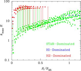
Figure 6: Consistency between the results of our stability analysis and the short-wavelength approximation, $k_{\mathrm{max}}R\gg 1$, where $k_{\mathrm{max}}$ is the least stable radial wavenumber, $R$ is the galactocentric distance, and $R_{25}$ is the optical radius. Large error bars signal a transition from star- to $\mathrm{H}_{2}$-dominated regimes, or vice versa, which causes a jump in the value of $k_{\mathrm{max}}$ (see Sect. 2).

Rather than estimating the magnitude and radial behaviour of $k_{\mathrm{max}}R$ with qualitative arguments, we plot this quantity as a function of galactocentric distance for all THINGS spirals analysed in Sect. 2. Fig. 6 illustrates that the results of our stability analysis are consistent with the short-wavelength approximation. For instance, the condition $k_{\mathrm{max}}R>3$ is fulfilled in 93% of the cases, and is always true for $R\ga 0.25\,R_{25}\approx R_{\mathrm{d}}$, i.e. at distances larger than about one disc scale length (remember that $R_{25}=4.6\pm 0.8\;R_{\mathrm{d}}$; L08). In contrast, there are only 2% of the data with $k_{\mathrm{max}}R\leq 1$, all close to the galactic centre: $R\la 0.05\,R_{25}\approx 0.25\,R_{\mathrm{d}}$. Such data correspond to star-dominated regimes, which are more prone to violate the short-wavelength approximation since $k_{\mathrm{max}}\sim\kappa/\sigma_{\star}$ and $\sigma_{\star}>\sigma_{\mathrm{HI}}>\sigma_{\mathrm{H2}}$. A comparison with the right panel of Fig. 4 shows that the corresponding values of $\mathcal{Q}_{3}$ are well above unity. As $\mathcal{Q}_{3}$ is well above unity and star-dominated in most of the cases, the few data with $k_{\mathrm{max}}R\leq 1$ do not have a significant influence on the stability of THINGS spirals. H i- and $\mathrm{H}_{2}$-dominated regimes are fully consistent with the short-wavelength approximation, and so are the corresponding values of $\mathcal{Q}_{3}$. In particular, the three data points that lie well below the critical stability level tell us that the nuclear region of NGC 6946 is subject to strong $\mathrm{H}_{2}$-dominated instabilities (see again the right panel of Fig. 4). This is consistent with the facts that NGC 6946 hosts a nuclear starburst (e.g., Engelbracht et al. 1996) and a nuclear ‘bar within bar’ (e.g., Fathi et al. 2007).

While the short-wavelength approximation is satisfied by most spiral galaxies, the assumption of axisymmetric (or tightly wound) perturbations is not so general. Local non-axisymmetric stability criteria are far more complex than Toomre’s criterion: they depend critically on how tightly wound the perturbations are, and cannot generally be expressed in terms of a single ‘effective’ $Q$ parameter (e.g., Lau & Bertin 1978; Morozov & Khoperskov 1986; Bertin et al. 1989b; Jog 1992; Lou & Fan 1998; Griv & Gedalin 2012). However, there is a general consensus that non-axisymmetric perturbations have a destabilizing effect, i.e. a disc with $Q\geq 1$ can still be locally unstable against such perturbations. Gas dissipation has a similar effect (Elmegreen 2011). These may be two of the reasons why the stability level of THINGS spirals is, on average, well above unity. The remarkable flatness of $\mathcal{Q}_{3\,\mathrm{med}}(R)$ across the entire optical disc is far more intriguing.

The assumption of local perturbations is quite controversial. While there is a general consensus that locally stable discs can be globally unstable as regards spiral structure formation, the dynamics and evolution of spiral structure depend critically on the radial profile of the $Q$ stability parameter (e.g., Bertin et al. 1989a, b; Lowe et al. 1994; Romeo 1994; Korchagin et al. 2000, 2005; Khoperskov et al. 2007; Sellwood 2011; Khoperskov et al. 2012). Our results about the stability level of THINGS spirals have no direct implications for that problem because they concern the THINGS sample as a whole, not each of the spirals. Useful constraints on the nature of spiral structure in galaxies might be found by analysing the radial profile of $\mathcal{Q}_{N}$ for each THINGS spiral, and by searching for trends in $\mathcal{Q}_{N}(R)$ along the Hubble sequence. This is however well beyond the scope of the present paper.

4 CONCLUSIONS

This paper provides a simple analytical recipe for estimating the $Q$ stability parameter in multi-component and realistically thick discs [see Eq. (19)]. Our $\mathcal{Q}_{N}$ parameter applies for any number of stellar and gaseous components ($i=1,\ldots,N$), and for the whole range of velocity anisotropy observed in galactic discs: $0\la(\sigma_{z}/\sigma_{R})_{i}\la 1$. The accuracy of this approximation can be rigorously quantified in the thin-disc limit, where it scales as $N^{-1/2}$. For $N=3$, the predicted root-mean-square error is well below 10%. This is true even for larger values of $N$. For example, in the ten-component model(s) of the Solar neighbourhood considered by Rafikov (2001) our approximation is accurate to within 5%. A further strength of the $\mathcal{Q}_{N}$ diagnostic is that it predicts which component dominates the local stability level. This is a useful piece of information, which should always be given when analysing the stability of galactic discs.

This paper also provides the first three-component analysis of THINGS spirals. Our analysis predicts how stars, H i and $\mathrm{H}_{2}$ contribute to disc (in)stability, and how the stability properties of such galaxies vary with galactocentric distance. We show that $\mathrm{H}_{2}$ plays a primary role up to distances of about one disc scale length. Stars dominate thereafter, but the contribution of $\mathrm{H}_{2}$ remains significant even at distances as large as half the optical radius. This is in sharp contrast to the role played by H i, which is negligible up to the edge of the optical disc. We also show that the stability level of THINGS spirals is, on average, remarkably flat and well above unity.

Appendix A DERIVATION OF EQ. (17)

From standard error analysis, we know that the relative uncertainty of $Q_{N}$ is approximately equal to that of $1/Q_{N}$:

$$\frac{\Delta Q_{N}}{Q_{N}}\sim\frac{\Delta(1/Q_{N})}{1/Q_{N}}$$ (20)

(see, e.g., Bevington & Robinson 2003). We also know that $\Delta(1/Q_{N})$ arises from estimation uncertainties in $W_{i}$ [see Eq. (15)]. If we assume that all $\Delta W_{i}$ are uncorrelated and of comparable magnitude, then the error propagation equation reduces to

$$\Delta(1/Q_{N})\sim\Delta W\left(\sum_{i=1}^{N}\frac{1}{Q_{i}^{2}}\right)^{1/2}\,.$$ (21)

Remembering that $Q_{i}\geq Q_{m}$, we get

$$\Delta(1/Q_{N})\la\frac{\Delta W}{Q_{m}}\,\sqrt{N}\,.$$ (22)

Noting that $1/Q_{N}>1/Q_{m}$ and using Eq. (A1), we then find

$$\frac{\Delta Q_{N}}{Q_{N}}\la\Delta W\,\sqrt{N}\,.$$ (23)

$\Delta W$ can be evaluated from the two-component case, where the root-mean-square value of the relative error $(Q_{2}-Q_{\mathrm{Rk}})/Q_{\mathrm{Rk}}$ is 5% (see Fig. 2). Setting $\Delta W\,\sqrt{2}\approx 0.05$, we finally obtain $\Delta W\approx 0.03$ and thus

$$\frac{\Delta Q_{N}}{Q_{N}}\la 0.03\,\sqrt{N}\,.$$ (24)

Appendix B THE TEN-COMPONENT CASES ANALYSED BY RAFIKOV (2001)

Table 2: Rafikov’s reference model of the Solar neighbourhood: surface densities and velocity dispersions of the various components.

$i$	Component	$\Sigma_{i}$ [M⊙ pc-2]	$\sigma_{i}$ [km s-1]
1	ISM	13.0	7.0
2	giants	0.4	26.0
3	$M_{V}<2.5$	0.9	17.0
4	$2.5<M_{V}<3.0$	0.6	20.0
5	$3.0<M_{V}<4.0$	1.1	22.5
6	$4.0<M_{V}<5.0$	2.0	26.0
7	$5.0<M_{V}<8.0$	6.5	30.5
8	$M_{V}>8.0$	12.3	32.5
9	white dwarfs	4.4	32.5
10	brown dwarfs	6.2	32.5

• Case 1: Rafikov’s reference model of the Solar neighbourhood. The epicyclic frequency is $\kappa=36\;\mbox{km\,s}^{-1}\,\mbox{kpc}^{-1}$. The surface densities and velocity dispersions of the various components are listed in Table B1.

• Case 2: same as Case 1, but with the velocity dispersion of white and brown dwarfs decreased from 32.5 to 20.0 km s^-1.

• Case 3: same as Case 1, but with the total surface density of white and brown dwarfs increased from 10.6 to 25.0 M_⊙ pc^-2.

• Case 4: same as Case 1, but with the gas velocity dispersion decreased from 7.0 to 5.9 km s^-1.

• Case 4+1: same as Case 1, but with the gas surface density increased from 13.0 to 14.8 M_⊙ pc^-2 (this case was only mentioned by Rafikov).

References

- [1] Agertz O., Lake G., Teyssier R., Moore B., Mayer L., Romeo A. B., 2009, MNRAS, 392, 294
- [2] Bertin G., Lin C. C., 1996, Spiral Structure in Galaxies: A Density Wave Theory. The MIT Press, Cambridge
- [3] Bertin G., Romeo A. B., 1988, A&A, 195, 105
- [4] Bertin G., Lin C. C., Lowe S. A., Thurstans R. P., 1989a, ApJ, 338, 78
- [5] Bertin G., Lin C. C., Lowe S. A., Thurstans R. P., 1989b, ApJ, 338, 104
- [6] Bevington P. R., Robinson D. K., 2003, Data Reduction and Error Analysis for the Physical Sciences. McGraw-Hill, Boston
- [7] Binney J., Tremaine S., 2008, Galactic Dynamics. Princeton University Press, Princeton
- [8] Cacciato M., Dekel A., Genel S., 2012, MNRAS, 421, 818
- [9] Ceverino D., Dekel A., Bournaud F., 2010, MNRAS, 404, 2151
- [10] Dalcanton J. J., Yoachim P., Bernstein R. A., 2004, ApJ, 608, 189
- [11] Dekel A., Sari R., Ceverino D., 2009, ApJ, 703, 785
- [12] Elmegreen B. G., 1995, MNRAS, 275, 944
- [13] Elmegreen B. G., 2011, ApJ, 737, 10
- [14] Elmegreen B. G., Scalo J., 2004, ARA&A, 42, 211
- [15] Elson E. C., de Blok W. J. G., Kraan-Korteweg R. C., 2012, AJ, 143, 1
- [16] Engelbracht C. W., Rieke M. J., Rieke G. H., Latter W. B., 1996, ApJ, 467, 227
- [17] Fathi K., Toonen S., Falcón-Barroso J., Beckman J. E., Hernandez O., Daigle O., Carignan C., de Zeeuw T., 2007, ApJ, 667, L137
- [18] Forbes J., Krumholz M., Burkert A., 2012, ApJ, 754, 48
- [19] Gerssen J., Shapiro Griffin K., 2012, MNRAS, 423, 2726
- [20] Griv E., Gedalin M., 2012, MNRAS, 422, 600
- [21] Hoffmann V., Romeo A. B., 2012, MNRAS, 425, 1511
- [22] Jog C. J., 1992, ApJ, 390, 378
- [23] Jog C. J., 1996, MNRAS, 278, 209
- [24] Jog C. J., Solomon P. M., 1984a, ApJ, 276, 114
- [25] Jog C. J., Solomon P. M., 1984b, ApJ, 276, 127
- [26] Khoperskov A. V., Just A., Korchagin V. I., Jalali M. A., 2007, A&A, 473, 31
- [27] Khoperskov S. A., Khoperskov A. V., Khrykin I. S., Korchagin V. I., Casetti-Dinescu D. I., Girard T., van Altena W., Maitra D., 2012, MNRAS, 427, 1983
- [28] Kim W.-T., Ostriker E. C., 2007, ApJ, 660, 1232
- [29] Korchagin V., Kikuchi N., Miyama S. M., Orlova N., Peterson B. A., 2000, ApJ, 541, 565
- [30] Korchagin V., Orlova N., Kikuchi N., Miyama S. M., Moiseev A., 2005, preprint (arXiv:astro-ph/0509708)
- [31] Lau Y. Y., Bertin G., 1978, ApJ, 226, 508
- [32] Leroy A. K., Walter F., Brinks E., Bigiel F., de Blok W. J. G., Madore B., Thornley M. D., 2008, AJ, 136, 2782
- [33] Li Y., Mac Low M.-M., Klessen R. S., 2005, ApJ, 626, 823
- [34] Li Y., Mac Low M.-M., Klessen R. S., 2006, ApJ, 639, 879
- [35] Lin C. C., Shu F. H., 1966, Proc. Natl. Acad. Sci. USA, 55, 229
- [36] Lou Y.-Q., Fan Z., 1998, MNRAS, 297, 84
- [37] Lowe S. A., Roberts W. W., Yang J., Bertin G., Lin C. C., 1994, ApJ, 427, 184
- [38] Mastropietro C., Burkert A., Moore B., 2009, MNRAS, 399, 2004
- [39] McKee C. F., Ostriker E. C., 2007, ARA&A, 45, 565
- [40] Meurer G. R., Zheng Z., de Blok W. J. G., 2013, MNRAS, 429, 2537
- [41] Morozov A. G., 1981, SvA, 7, L5
- [42] Morozov A. G., Khoperskov A. V., 1986, Ap, 24, 266
- [43] Press W. H., Teukolsky S. A., Vetterling W. T., Flannery B. P., 1992, Numerical Recipes in Fortran: The Art of Scientific Computing. Cambridge University Press, Cambridge
- [44] Rafikov R. R., 2001, MNRAS, 323, 445
- [45] Robertson B. E., Kravtsov A. V., 2008, ApJ, 680, 1083
- [46] Romeo A. B., 1985, Stabilità di Sistemi Stellari in Presenza di Gas: Fenomeni Collettivi in Sistemi Autogravitanti a Due Componenti. Tesi di Laurea, University of Pisa and Scuola Normale Superiore, Pisa, Italy
- [47] Romeo A. B., 1990, Stability and Secular Heating of Galactic Discs. PhD thesis, SISSA, Trieste, Italy
- [48] Romeo A. B., 1992, MNRAS, 256, 307
- [49] Romeo A. B., 1994, A&A, 286, 799
- [50] Romeo A. B., Wiegert J., 2011, MNRAS, 416, 1191
- [51] Romeo A. B., Burkert A., Agertz O., 2010, MNRAS, 407, 1223
- [52] Sellwood J. A., 2011, MNRAS, 410, 1637
- [53] Shadmehri M., Khajenabi F., 2012, MNRAS, 421, 841
- [54] Shen Y., Lou Y.-Q., 2003, MNRAS, 345, 1340
- [55] Shu F. H., 1968, The Dynamics and Large Scale Structure of Spiral Galaxies. PhD thesis, Harvard University, Cambridge, Massachusetts, USA
- [56] Toomre A., 1964, ApJ, 139, 1217
- [57] Watson L. C., Martini P., Lisenfeld U., Wong M.-H., Böker T., Schinnerer E., 2012, ApJ, 751, 123
- [58] Westfall K. B., Bershady M. A., Verheijen M. A. W., Andersen D. R., Martinsson T. P. K., Swaters R. A., Schechtman-Rook A., 2011, ApJ, 742, 18
- [59] Williamson D. J., Thacker R. J., 2012, MNRAS, 421, 2170
- [60] Wilson C. D. et al., 2011, MNRAS, 410, 1409
- [61] Yang C.-C., Gruendl R. A., Chu Y.-H., Mac Low M.-M., Fukui Y., 2007, ApJ, 671, 374
- [62] Yim K., Wong T., Howk J. C., van der Hulst J. M., 2011, AJ, 141, 48
- [63] Zheng Z., Meurer G. R., Heckman T. M., Zwaan M., 2013, MNRAS, submitted