Disentangling glass and jamming physics in the rheology of soft materials

Abstract

The shear rheology of soft particles systems becomes complex at large density because crowding effects may induce a glass transition for Brownian particles, or a jamming transition for non-Brownian systems. Here we successfully explore the hypothesis that the shear stress contributions from glass and jamming physics are ‘additive’. We show that the experimental flow curves measured in a large variety of soft materials (colloidal hard spheres, microgel suspensions, emulsions, aqueous foams) as well as numerical flow curves obtained for soft repulsive particles in both thermal and athermal limits are well described by a simple model assuming that glass and jamming rheologies contribute linearly to the shear stress, provided that the relevant scales for time and stress are correctly identified in both sectors. Our analysis confirms that the dynamics of colloidal hard spheres is uniquely controlled by glass physics while aqueous foams are only sensitive to jamming effects. We show that for micron-sized emulsions both contributions are needed to successfully account for the flow curves, which reveal distinct signatures of both phenomena. Finally, for two systems of soft microgel particles we show that the flow curves are representative of the glass transition of colloidal systems, and deduce that microgel particles are not well suited to studying the jamming transition experimentally.

I Introduction

The emergence of solidity in disordered assemblies of soft particles is observed in large variety of systems, everyday examples including toothpaste, shaving foam, or paints larson ; coussot . Because of their practical use, a fundamental understanding of the flow property of dense suspensions is necessary, but this continues to represent a considerable challenge to physicists. In particular, achieving a detailed understanding of fluid-to-solid transitions in amorphous materials is recognized as an important challenge for modern condensed matter physics rmp ; jammingrev .

Two types of dense particulate systems have been considered. One class is composed of particles that are small enough to be sensitive to thermal fluctuations. Brownian forces are for instance relevant in colloidal suspensions of micron-sized particles or smaller. In that case, colloids undergo collisions with the solvent molecules which play the role of a thermal bath. The emergence of amorphous solids at large density in such materials is usually called colloidal glass transition pusey , by analogy with the molecular glass transition observed in organic or polymeric liquids rmp .

In a second class of systems thermal fluctuations play a negligible role, with aqueous foams being one example. In these non-Brownian systems, the particle size is typically very large (say, in the millimeter range), such that the effect of collisions with solvent molecules is so weak that it can be safely neglected on typical experimental timescales. The emergence of solidity in athermal amorphous systems was termed jamming transition liunagel , by analogy with dry granular media grains .

Surprisingly, despite large differences in the underlying microscopic dynamics, the phenomenology of glass and jamming transitions appears remarkably similar, in particular when soft particle systems are considered ohern1 ; vanhecke . Below some critical density, the system can flow under infinitesimal shear stress. The nature of the flow is Newtonian, and the system thus behaves as a viscous fluid. Above that critical density, the system does not flow if the shear stress is below a characteristic finite value, called the yield stress. The system is now a soft solid. Close to the critical density, the rheology is typically strongly non-linear: it is very sensitive to small density changes, and the microscopic dynamics becomes spatially and temporally heterogeneous book .

This apparent similarity suggests that theoretical progress for one type of systems might impact research for the other. For Brownian systems, flow curves are typically analyzed by assuming that the glassy dynamics arising in thermal suspensions at rest is disrupted by the externally imposed shear flow yamamoto ; BBK ; BB ; fuchs . A number of experimental studies, in particular in the colloidal literature, have then used these ideas to organize and quantitatively describe flow curves measured in the vicinity of the glass transition exp1 . By contrast, much less is understood regarding the microscopic dynamics of athermal suspensions near the jamming transition, because the imposed shear flow represents at the same time the external driving force and the source of microscopic fluctuations responsible for particle motion. Nevertheless, detailed numerical analysis of model systems and theoretical modelling have suggested specific functional forms and scaling procedures to organize rheological data around the jamming transition olson ; tighe ; olson2 ; lerner . In fact these ideas have been used in a larger variety of systems, including atomistic glasses egami and colloidal particles yodh , where their relevance is not obvious a priori.

Recently, we have used numerical simulations to study the rheology of dense assemblies of soft repulsive spheres letter . Despite its simplicity, this model is useful as it is known to display glassy dynamics at finite temperatures tom , and to undergo a geometric jamming transition at zero temperature ohern1 ; durian . By varying the relative strength of energy dissipation and thermal agitation over a broad range, we have demonstrated that glass and jamming physics impact the steady state flow curves over distinct stress scales and time scales, which can be varied independently. These results confirm that the two phenomena are actually distinct, and that their respective influences on rheological behaviour should not be confused. In addition, we have suggested that the numerical flow curves are well described by a simple ‘additive’ model, where the glass and jamming contributions to the shear stress can be captured separately and then combined linearly into a unified model letter .

In the present work, we expand our presentation of this additive model to explain in greater detail its construction and application to our numerical data. We then confront our rheological model deduced from the analysis of a simplistic soft particle system to a broad range of experimental data taken from the literature. Overall, our analysis validates the hypothesis that, despite their strongly nonlinear nature, glass and jamming physics linearly contribute to the rheology of soft particle systems and act over distinct sectors, whose relative importance depends on the experimental system at hand. We also show that our model and theoretical analysis provide useful tools to organize and explain rheological data stemming from different experimental sources and materials. These tools can be used to efficiently identify which of the glass or jamming contributions is most relevant, or whether both types of physics are in fact needed to correctly describe the data.

Our paper is organized as follows. In Sec. II we construct our additive rheological model which we apply to numerical data obtained from simulations of harmonic spheres. In Sec. III we use this model to analyze steady state flow curves measured in colloidal hard spheres, microgel suspensions, emulsions, and aqueous foams. In Sec. IV, we summarize our findings and discuss some perspectives for future work.

II ‘Additive’ model for glass and jamming rheology

II.1 Flow curves for harmonic spheres

To construct a general model for the complex rheology of dense suspensions, we use the numerical results obtained for a specific model as a reference. In previous work, we have studied the steady state rheology of harmonic spheres in the overdamped limit letter . This can be seen as a simple model to describe the physical behavior of dense suspensions of deformable spheres, such as the emulsions and colloidal suspensions considered in Sec. III.

Since the details of the model were already reported in our previous work, we only briefly summarize the key ingredients. We consider $N$ harmonic spheres contained in a volume $V$. We use Lees-Edwards periodic boundary conditions allen and solve the following equations of motion numerically:

$$\xi(\frac{\partial\vec{r}_{i}}{\partial t}-\dot{\gamma}y_{i}\vec{e}_{x})=-\sum_{j=1}^{N}\frac{\partial v(|\vec{r}_{i}-\vec{r}_{j}|)}{\partial\vec{r}_{i}}+\vec{R}_{i}.$$ (1)

Here $\vec{r}_{i}$ represents the position of particle $i$, $y_{i}$ its $y$-component, and $\vec{e}_{x}$ the unit vector along the $x$-axis. The damping coefficient, $\xi$, and the random force, $\vec{R}_{i}(t)$, obey the fluctuation dissipation relation: $\langle{\vec{R}_{i,\alpha}(s)\vec{R}_{j,\beta}(s^{\prime})}\rangle=2k_{B}T\xi\delta_{ij}\delta_{\alpha\beta}\delta(s-s^{\prime})$, where $T$ is the temperature and $k_{B}$ is Boltzmann’s constant. The interaction potential is a purely repulsive harmonic interaction truncated at the particle diameter,

$$v(r)=\frac{\epsilon}{2}\left(1-\frac{r}{a}\right)^{2}\,\Theta(r-a),$$ (2)

where $a$ is the particle diameter and $\Theta(x)$ is the Heaviside function. To avoid crystallization issues, we work with a 50:50 binary mixture of particles with diameter ratio 1.4, but this is otherwise largely irrelevant.

By construction, the system has two characteristic energy scales, namely the thermal energy, $k_{B}T$, and the interaction energy of particles $\epsilon$. The ratio of these energy scales, $k_{B}T/\epsilon$, is an important control parameter. Physically, it is a measure of the particle softness, expressed in units of kinetic energy.

Glass and jamming effects can be distinguished most clearly in the low-softness limit $k_{B}T/\epsilon\to 0$. This can be obtained in two ways. One can either take the limit of vanishing kinetic energy, $T\to 0$, at fixed repulsion energy scale $\epsilon$. One then studies the jamming transition of athermal packings of soft repulsive spheres. The alternative is to keep temperature constant and send $\epsilon\to\infty$, a limiting case which corresponds to studying the physics of the thermalized hard sphere fluid.

The two energy scales $k_{B}T$ and $\epsilon$ naturally provide two characteristic time scales and stress scales. The microscopic time scale for Brownian motion is

$$\tau_{\rm T}=\frac{\xi a^{2}}{k_{B}T},$$ (3)

and represents the time it takes a particle to diffuse by Brownian motion over a length scale comparable to its size. The characteristic time scale for energy dissipation is given by

$$\tau_{0}=\frac{\xi a^{2}}{\epsilon}=\frac{k_{B}T}{\epsilon}\tau_{\rm T}.$$ (4)

Likewise, we can define two stress scales: a typical stress created by thermal fluctuations,

$$\sigma_{\rm T}=\frac{k_{B}T}{a^{3}},$$ (5)

and an athermal stress scale:

$$\sigma_{0}=\frac{\epsilon}{a^{3}}=\frac{k_{B}T}{\epsilon}\sigma_{\rm T}.$$ (6)

The above expressions make it clear that these time scales and stress scales are comparable when particle softness is large enough, ${k_{B}T}\approx{\epsilon}$, while they become increasingly separated as the athermal limit is approached, ${k_{B}T}\ll{\epsilon}$.

In terms of the time and stress scales above we can now give a more explicit statement of when the limit $k_{B}T/\epsilon\to 0$ corresponds to athermal or thermal behaviour. If the limit is taken by lowering $T$ at constant $\epsilon$ then the shear rate in athermal units, $\dot{\gamma}\tau_{0}$, stays fixed: we are exploring the ‘athermal sector’. Here we then also expect stresses to be on the athermal scale, with $\sigma/\sigma_{0}$ of order unity. If on the other hand we fix $T$ and take $\epsilon\to\infty$, then the shear rate on the thermal scale, $\dot{\gamma}\tau_{T}$, remains finite. One then probes the ‘thermal sector’, with correspondingly $\sigma/\sigma_{T}=O(1)$. Numerically, we find (see below) that the prefactors in these estimates are such that, below and around the glass transition, the interesting physics typically takes place for $\dot{\gamma}\tau_{T}<1$ and $\sigma/\sigma_{T}<1$. As a matter of general orientation we can therefore say that phenomena where the shear rate and stress in thermal units are below unity belong to the thermal sector, while the athermal sector corresponds to values of these quantities significantly above one. A numerical analysis along the same lines has appeared recently olson3 .

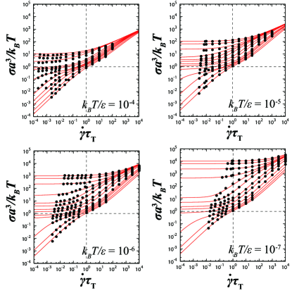
Figure 1: Flow curves of harmonic spheres for temperatures from $k_{B}T/\epsilon=10^{-4}$ down to $10^{-7}$ measured in the simulations first described in Ref. letter (symbols). In each panel, packing fraction increases from bottom to top in the range $\varphi=0.55-0.70$. The red lines are fits using the additive model presented in this work, with parameters listed in Table 1. The dashed lines delimit the thermal/glass (bottom left) and athermal/jamming (top right) sectors.

In Fig. 1 we present flow curves obtained by measuring the average shear stress, $\sigma$, under steady state conditions created by a constant applied shear rate, $\dot{\gamma}$, and varying the packing fraction, $\varphi$, and the temperature, $T$, across a broad range. Note that we use stresses and shear rates normalized by $\tau_{\rm T}$ and $\sigma_{\rm T}$ as time and stress units; these are the appropriate scales for thermal systems. This leads us to introduce a ‘renormalized’ shear rate,

$$P_{\rm e}=\dot{\gamma}\tau_{\rm T},$$ (7)

which is also called the Péclet number. Because the results shown in Fig. 1 were discussed in detail in Ref. letter , we only summarize the most salient features of these data.

• High temperature / Soft particles (such as $k_{B}T/\epsilon=10^{-4}$). A single fluid-to-solid transition is observed in this thermal regime. When the density is low, Newtonian flow is observed at low shear rates $\dot{\gamma}\ll\tau_{\rm T}^{-1}$. With increasing density, the Newtonian viscosity grows and a shear stress plateau appears at finite shear rate, corresponding to a strong shear-thinning regime. Near the transition density, $\varphi\approx\varphi_{\rm G}$, the viscosity becomes very large, and a finite yield stress appears, which grows smoothly with density upon further compression.

• Low temperature / Hard particles (such as $k_{B}T/\epsilon=10^{-7}$). The glass and jamming transition can be observed separately. When the density is low, two Newtonian regimes appear for $\dot{\gamma}\ll\tau_{\rm T}^{-1}$ and $\tau_{\rm T}^{-1}\ll\dot{\gamma}\ll\tau_{0}^{-1}$, respectively. The first Newtonian viscosity becomes very large near the glass transition density $\varphi_{\rm G}$ where the system acquires a finite yield stress, of the order of the thermal stress scale $\sigma_{\rm T}$. However the second Newtonian viscosity remains finite at the glass transition density. On further increasing the density, the second Newtonian viscosity then diverges at the jamming transition density $\varphi_{\rm J}$. At the same time, the yield stress value increases rapidly with density; above the jamming transition it reaches a value which is controlled by the athermal stress scale $\sigma_{0}$.

These numerical results directly illustrate that glass and jamming transitions represent distinct ways for the system to form an amorphous solid phase, since the fluid-to-solid transitions occur over different time windows (or, equivalently, different shear rates) and give rise to solids with yield stress having different scales and different physical origins. By tuning the temperature of our system, we can move from Brownian soft particles undergoing a glass transition in the thermal sector of Fig. 1 to non-Brownian ones undergoing a geometric jamming transition in a different sector. Interestingly, both types of physics compete and affect the flow curves for intermediate values of the temperatures. These observations indicate that the particle softness, $k_{B}T/\epsilon$, is a central control parameter for the rheology of soft materials. In particular, we note that when the particles are too soft (equivalently, when temperature is too large), the jamming transition has no effect on the rheological data.

II.2 Construction of an additive model

II.2.1 The additive hypothesis

Using the simulation results as a reference, we now construct a simple rheological model. The major assumption is the additivity of the contributions from thermal and athermal parts to the total shear stress:

$$\sigma(T,\varphi,\dot{\gamma})=\sigma_{\rm G}(T,\varphi,\dot{\gamma})+\sigma_{\rm J}(\varphi,\dot{\gamma})+\eta_{\rm s}\dot{\gamma}.$$ (8)

Here $\sigma_{\rm G}$ is the thermal part of the stress describing the physics of the glass transition, while $\sigma_{\rm J}$ is the athermal part of the stress accounting for the jamming transition. Finally, $\eta_{s}$ is the solvent viscosity, so that $\eta_{s}\dot{\gamma}$ is the stress stemming from the background solvent. This only becomes relevant in the dilute limit but serves as a useful reference value when considering experimental data.

Our goal with the model in Eq. (8) is not to make new types of predictions for the functional form of the flow curves for systems near glass and jamming transitions, but rather to explore the interplay between both physics. Thus, we make use of previous theoretical work and choose simple functional forms that most efficiently capture the physical features of the flow curves associated with each of these transitions.

II.2.2 The glass contribution

First, we specify the thermal part of the stress, $\sigma_{\rm G}$. We write it as the sum of the zero and the finite shear rate parts:

$$\frac{\sigma_{\rm G}(T,\varphi,\dot{\gamma})}{\sigma_{\rm T}} = \sigma_{\rm GY}(\varphi)+$$

$$\frac{Y_{\rm G}}{(\dot{\gamma}\tau_{\rm T}G(\varphi))^{-1}+(1+p_{\rm G}(\dot{\gamma}\tau_{\rm T})^{\alpha_{\rm G}})^{-1}}.$$

Although compact, this expression incorporates quite a number of physical features of the rheology of glass-forming suspensions. In this equation, $Y_{\rm G}$ and $p_{\rm G}$ are two dimensionless numerical prefactors, with no deep information content. This expression is constructed to produce flow curves with no yield stress (defined as the $\dot{\gamma}\to 0$ limit value of the shear stress) at low density, and a finite value for the glass phase when density is larger than the glass transition density, $\varphi_{\rm G}$, which is assumed to be sharply defined. This last point is discussed further in Sections II.3 and II.5 below.

We note to start with that the shear rate and shear stress in Eq. (II.2.2) are expressed in units appropriate for Brownian suspensions, namely $\sigma_{\rm T}$ and $\tau_{\rm T}$. It is mainly via these elementary units $\tau_{\rm T}$ and $\sigma_{\rm T}$ that the temperature dependence of the flow curves enters (apart from a minor temperature dependence of the transition density, see Sec. II.3 below). The microscopic expressions of these units are given by Eqs. (3, 5) for a system obeying Langevin dynamics, as in our numerical simulations. In experiments, one might want to replace the damping coefficient $\xi$ in this expression using instead Stokes’ law to obtain the microscopic time scale:

$$\tau_{\rm T}=\frac{3\pi\eta_{\rm s}a^{3}}{k_{B}T}.$$ (10)

Having set the correct scales, we now describe the functional form of the flow curves predicted by Eq. (II.2.2). For densities below the glass transition, $\varphi<\varphi_{\rm G}$, the yield stress is zero, and we impose accordingly $\sigma_{\rm GY}(\varphi\leq\varphi_{\rm G})=0$. Thus, only the second term on the right hand side needs to be discussed. For small shear rates, $\dot{\gamma}\ll(\tau_{\rm T}G(\varphi))^{-1}$, the first term in the denominator dominates and the equation becomes $\sigma_{\rm G}\approx Y_{\rm G}\sigma_{\rm T}\tau_{\rm T}G(\varphi)\dot{\gamma}$. This represents Newtonian behavior with the thermal viscosity $\eta_{\rm T}(\varphi)$ given by

$$\eta_{\rm T}(\varphi)\equiv 3\pi Y_{\rm G}G(\varphi)\eta_{s}.$$ (11)

This expression shows that the dimensionless function $G(\varphi)$ controls the rapid growth of the viscosity on approaching the glass transition, and thus also corresponds to the growing equilibrium relaxation time of the unsheared Brownian suspension at density $\varphi$, via the relation $\tau_{\alpha}\approx G(\varphi)\tau_{\rm T}$.

At larger shear rates, the flow curve (II.2.2) becomes $\sigma_{\rm G}\approx Y_{\rm G}\sigma_{\rm T}(1+p_{\rm G}(\dot{\gamma}\tau_{\rm T})^{\alpha_{\rm G}})$; here we assume that the exponent $\alpha_{\rm G}$ takes a value below unity. This expression describes the strong shear-thinning regime obtained in dense fluids when the shear rate competes with the slow glassy dynamics and drives the system away from equilibrium. This competition is modelled by a plateau regime, $\sigma_{\rm G}\approx Y_{G}\sigma_{\rm T}$, when $\dot{\gamma}\ll\tau_{\rm T}^{-1}$, finally followed by a different shear-thinning behaviour, $\sigma_{\rm G}\approx Y_{G}p_{\rm G}\sigma_{\rm T}(\dot{\gamma}\tau_{\rm T})^{\alpha_{\rm G}}$. These two shear-thinning regimes result from the well-known existence of two separated relaxation processes ($\alpha$ and $\beta$ relaxations) in highly viscous fluids thomas .

In the glass phase, $\varphi>\varphi_{G}$, we impose an infinite value of the Newtonian viscosity using $G(\varphi)=\infty$, such that the first term in the denominator disappears from Eq. (II.2.2) and the flow curve simplifies to $\sigma_{\rm G}/\sigma_{\rm T}=[Y_{\rm G}+\sigma_{\rm GY}(\varphi)]+Y_{\rm G}p_{\rm G}(\dot{\gamma}\tau_{\rm T})^{\alpha_{\rm G}}$. This describes the existence of a finite yield stress,

$$\sigma^{\rm yield}=\left[Y_{\rm G}+\sigma_{\rm GY}(\varphi)\right]\sigma_{\rm T},$$ (12)

whose scale is set by the thermal stress. At finite shear rates the rheology is of Herschel-Bulkley type larson , with shear-thinning exponent $\alpha_{\rm G}$.

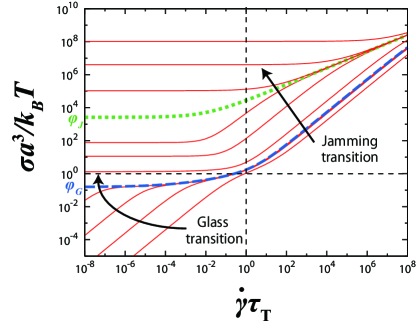
Figure 2: Flow curves predicted by the additive model at low temperatures, $k_{B}T/\epsilon=10^{-10}$, when glass (bottom left) and jamming (top right) sectors are well separated. Notice the different functional forms of the flow curves near the critical densities $\varphi_{\rm G}$ and $\varphi_{\rm J}$ (highlighted with dashed and dotted lines), reflecting the distinct microscopic dynamics associated with thermal and athermal situations.

The resulting functional forms for the glass contribution are shown graphically in the bottom left sector of Fig. 2, which corresponds to the thermal sector of the rheology predicted by the present model. We defer a discussion of the volume fraction dependences of $\sigma_{\rm GY}$ and $G$ to Sec. II.3 below.

II.2.3 The jamming contribution

We now turn to the jamming contribution to the shear stress in Eq. (8), $\sigma_{\rm J}$. We express this athermal part of the stress as:

$$\frac{\sigma_{\rm J}(\varphi,\dot{\gamma})}{\sigma_{0}}=\sigma_{\rm JY}(\varphi)+\frac{Y_{\rm J}}{(\dot{\gamma}\tau_{0}J(\varphi))^{-1}+(p_{\rm J}(\dot{\gamma}\tau_{0})^{\alpha_{\rm J}})^{-1}}$$ (13)

In this expression, we have introduced two dimensionless parameters, $Y_{\rm J}$ and $p_{\rm J}$. In contrast to the glass contribution, the stress and time units are now $\sigma_{0}$ and $\tau_{0}$, whose microscopic expressions were given in Eqs. (4, 6). Therefore, temperature does not enter the stress contribution (13), as expected from the athermal nature of jamming physics.

Expression (13) has many similarities with Eq. (II.2.2) but is qualitatively slightly simpler, as we now describe. For densities below the jamming density, we impose $\sigma_{\rm JY}(\varphi\leq\varphi_{\rm J})=0$, such that a Newtonian viscosity emerges in the low shear rate limit, $\dot{\gamma}\ll(\tau_{0}J(\varphi))^{-1}$. Here $\sigma_{\rm J}\approx Y_{\rm J}\sigma_{0}\tau_{0}J(\varphi)$, which defines the athermal viscosity

$$\eta_{0}(\varphi)\equiv 3\pi Y_{\rm J}J(\varphi)\eta_{s}.$$ (14)

This equation shows that the dimensionless function $J(\varphi)$ now controls the divergence of the Newtonian viscosity on appraoching $\varphi_{\rm J}$. The difference with the glass regime is seen at larger shear rates because the constant contribution in the denominator of Eq. (II.2.2) is absent in Eq. (13). As a result, Eq. (13) shows a simple power law shear-thinning behavior $\sigma_{\rm J}\approx Y_{\rm J}\sigma_{0}p_{\rm J}(\dot{\gamma}\tau_{0})^{\alpha_{\rm J}}$, instead of the plateau in Eq. (II.2.2). This reflects the absence of distinct $\alpha$ and $\beta$ relaxations in athermal systems letter .

In the jammed phase, $\varphi>\varphi_{\rm J}$, we impose a nonzero yield stress, $\sigma_{\rm JY}>0$, and an infinite viscosity via $J(\varphi)=\infty$. As a result, we obtain $\sigma_{\rm J}/\sigma_{0}=\sigma_{\rm JY}(\varphi)+Y_{\rm J}p_{J}(\dot{\gamma}\tau_{0})^{\alpha_{\rm J}}$, which describes the existence of a finite yield stress,

$$\sigma^{\rm yield}=\sigma_{\rm JY}(\varphi)\,\sigma_{0}.$$ (15)

Its units are given by the athermal stress. Again at finite shear rates we have Herschel-Bulkley rheology, with the shear-thinning exponent now $\alpha_{\rm J}$.

The resulting functional forms for the jamming contribution are shown graphically in the top right quadrant of Fig. 2, which corresponds to the athermal sector of the rheology predicted by the present model.

II.3 Density dependence: Choice of fitting functions

In both thermal and athermal expressions for the shear stress, we have described a change from fluid to solid behaviour signalled by rapidly growing viscosities controlled by the dimensionless functions $G(\varphi)$ and $J(\varphi)$, and emerging yield stresses controlled by the functions $\sigma_{\rm GY}(\varphi)$ and $\sigma_{\rm JY}(\varphi)$. Within our model, these functions entirely control the density dependence of the flow curves. In this subsection, we describe the physics embodied by these quantities, and motivate the specific choices we made to fit numerical and experimental flow curves in the present paper.

II.3.1 Diverging Newtonian viscosities

For thermal systems, the function $G(\varphi)$ controlling the growth of the Newtonian viscosity has been carefully analyzed in a large number of studies, as it quantifies the dynamic slowing down of a hard sphere fluid on its approach to the colloidal glass transition pusey ; chaikin ; bill ; gio . As is well known from the literature of glass-forming materials rmp , this timescale growth cannot be represented by a single functional form because the slowing down of the dynamics crosses over from power law timescale increase at moderate volume fraction, to a steeper ‘activated’ exponential growth at larger density gio . This crossover can be understood theoretically as a change of relaxation mechanism from collective but nonactivated dynamics described by mode-coupling theory gotze , to correlated activated events closer to the glass transition rmp .

In practice, however, given the limited range of viscosity data that is accessible in typical numerical and experimental work, a single functional form is often a good enough approximation to describe the data. Therefore, in the following we shall describe the data using a power law divergence:

$$G(\varphi)=h_{\rm G}(\varphi_{\rm G}-\varphi)^{-\gamma_{\rm G}},$$ (16)

where $h_{\rm G}$ is a numerical prefactor. The location of the glass transition, $\varphi_{\rm G}$, and the associated exponent, $\gamma_{\rm G}$, are fit parameters that serve to describe the increase with density of the thermal viscosity $\eta_{\rm T}(\varphi)$. As is clear from the above description, the value extracted for the location of the glass transition has the same physical content as the location of the mode-coupling temperature for standard glass-forming materials; it should not be confused with the location of a genuine dynamic or thermodynamic singularity tom2 .

On the other hand, much less is known about the density dependence of the athermal viscosity $\eta_{0}$, controlled in our model by the dimensionless function $J(\varphi)$. Theoretical olson ; lerner and experimental lindner ; boyer studies seem to indicate that a power law divergence describes the results well, and accordingly we use

$$J(\varphi)=h_{\rm J}(\varphi_{\rm J}-\varphi)^{-\gamma_{\rm J}},$$ (17)

with $h_{\rm J}$ a numerical prefactor. The exponent $\gamma_{\rm J}$ is found numerically and experimentally to be close to $\gamma_{\rm J}=2$. The critical density, $\varphi_{\rm J}$, appearing in the expression (17) represents the location of the jamming transition.

Although Eqs. (16, 17) appear similar, we note that the former has been derived from a microscopic perspective gotze , while the second one is only supported by experimental data or detailed theoretical and numerical analysis performed over a limited range of densities lerner ; boyer . Therefore, while empirically robust, the status of the algebraic divergence for non-Brownian hard sphere suspensions remains to be clarified. A second difference between the two expressions concerns the nature of the critical densities. While we described $\varphi_{\rm G}$ as the crossover density emerging from a mode-coupling theory analysis of the data, an actual divergence is expected in the athermal limit, such that $\varphi_{\rm J}$ is not simply a crossover but a genuine critical density jammingrev . However, its location remains ambiguous: the nonequilibrium nature of the jamming transition implies that it depends on the specific details of the procedure used to bring a system close to jamming donev . This implies, for instance, that the values for $\varphi_{\rm J}$ obtained by slow or fast compressions of random sphere packings do not coincide with the critical density measured under shear pinaki . Thus, $\varphi_{\rm J}$ in Eq. (17) is very specifically defined as the critical density that controls the divergence of the Newtonian viscosity of non-Brownian particles in the hard sphere limit olson ; lerner .

II.3.2 Emerging yield stress

We now discuss the behaviour of the yield stress for glass and jammed phases, which is also characterized by a number of singular behaviours, as demonstrated by the numerical measurements performed on harmonic spheres at various temperatures and reported in Fig. 3. These yield stress data are obtained from the zero shear rate extrapolation of the flow curves shown in Fig. 1.

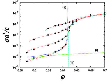
Figure 3: Yield stress of harmonic spheres, measured numerically at $k_{B}T/\epsilon=10^{-4}$, $10^{-5}$, $10^{-6}$ and $10^{-7}$ (from top to bottom). These results are extracted from the $\dot{\gamma}\to 0$ limit of the flow curves in Fig. 1. The red lines are fits using Eqs. (21, 22). The three lines for $T=10^{-7}$ represent fits to the simpler functional forms in Eq. (18) [(i), dashed], Eq. (19) [(ii), dash-dotted], and Eq. (20) [(iii), dotted].

As can be seen from Fig. 3, the yield stress data show three distinct characteristic behaviours, which are more or less pronounced depending on temperature, and thus one can use various levels of sophistication in the description of these data.

The first observation is related to the appearance and growth with density of a yield stress above the glass transition $\varphi_{\rm G}$. Within our model, this behaviour is controlled by the term $\sigma_{\rm GY}(\varphi)$, see Eq. (12). A possible functional form is

$$\sigma_{\rm GY}(\varphi\geq\varphi_{\rm G})=A_{\rm G}(\varphi-\varphi_{\rm G})^{\beta_{\rm G}},$$ (18)

where $A_{\rm G}$ is a prefactor and $\beta_{\rm G}$ an exponent which characterizes the growth of the yield stress with density. This form is consistent with the description provided by the extension of the mode-coupling theory to sheared suspensions fuchs , where the exponent is given by $\beta_{\rm G}=\frac{1}{2}$. The data in Fig. 3 indicate that Eq. (18) is sufficient to describe the yield stress of harmonic spheres when the temperature is high enough, e.g. $k_{B}T=10^{-4}$, so that the jamming transition does not play any role. Note, however, that a precise determination of the exponent in Eq. (18) is not possible, as it is difficult to obtain unambiguous yield stress data very near $\varphi_{\rm G}$ due to the crossover nature of the mode-coupling transition: the flow curve at the fitted $\varphi_{\rm G}$ would eventually become Newtonian at low enough shear rates.

By contrast, the jamming density becomes relevant when temperatures becomes much smaller, and this affects the yield stress on both sides of the jamming transition. For $\varphi<\varphi_{\rm J}$ and $T\to 0$ the behaviour of hard sphere glasses is recovered, for which the yield stress diverges as $\varphi_{\rm J}$ is approached from below bookmewis . One can model this behaviour using again an algebraic dependence,

$$\sigma_{\rm GY}(\varphi\leq\varphi_{\rm J})=B_{\rm G}(\varphi_{\rm J}-\varphi)^{-\beta_{\rm GJ}},$$ (19)

where $B_{\rm G}$ is a numerical prefactor. We are not aware of specific theoretical predictions for the value of the exponent $\beta_{\rm GJ}$ governing the yield stress divergence, but one might expect that it is the same exponent which also controls the divergence of the pressure in compressed hard spheres, for which the value $\beta_{\rm GJ}=1$ is well documented tom2 ; freevol ; wood .

The third characteristic density dependence is obtained above the jamming transition in the $T\to 0$ limit. In our model this is entirely controlled by the term $\sigma_{\rm JY}$; see Eq. (15). The emergence of a yield stress in athermal soft sphere packings has been described in previous numerical work as a continuous power law growth durian ; olson ,

$$\sigma_{\rm JY}(\varphi\geq\varphi_{\rm J})=Y_{\rm J}(\varphi-\varphi_{\rm J})^{\beta_{\rm J}}.$$ (20)

Note that there is no need to introduce a new prefactor in this expression, as the second term of Eq. (13) already contains two adjustable prefactors in the denominator, $p_{\rm J}$ and $h_{\rm J}$ from $J(\varphi)$. The expression (20) is known to be sufficient when describing fully athermal assemblies of soft particles olson . The exponent $\beta_{\rm J}$ has been found to be close to $\beta_{\rm J}=1$, although small deviations from this simple value of $\beta_{\rm J}$ have also been discussed olson .

We have represented the three fitting functions in Eqs. (18, 19, 20) as lines going through the numerical results in Fig. 3, demonstrating that each of these expressions can describe a limited range of densities fairly well; each therefore correctly captures a different physical regime of the yield stress behaviour of harmonic spheres.

However, as is clear from Fig. 3, for finite but very low temperatures all three regimes affect the density dependence of the yield stress. Therefore, to describe the functional form of such low-$T$ data correctly one must introduce more complicated model equations that interpolate smoothly between the various regimes. A possible expression is as follows:

$$\sigma_{\rm GY}=\frac{1}{Y_{\rm GJ}^{-1}\sqrt{\frac{\sigma_{T}}{\sigma_{0}}}+Y_{\rm G}^{\prime-1}(\varphi-\varphi_{\rm G})^{-\beta_{\rm G}}(\varphi_{\rm J}-\varphi)^{\beta_{\rm GJ}}},\quad$$ (21)

$$\sigma_{\rm JY}=Y_{\rm GJ}\sqrt{\frac{\sigma_{\rm T}}{\sigma_{0}}}+Y_{\rm J}(\varphi-\varphi_{\rm J})^{\beta_{\rm J}}.$$ (22)

In these equations we have used the product $Y_{\rm G}^{\prime}(\varphi-\varphi_{\rm G})^{\beta_{\rm G}}(\varphi_{\rm J}-\varphi)^{-\beta_{\rm GJ}}$ in the thermal part to interpolate continuously between expressions (18) and (19) in between the glass and jamming transition densities. This has the added benefit of reducing the number of adjustable numerical prefactors by one, by effectively replacing $A_{\rm G}$ and $B_{\rm G}$ with $Y_{\rm G}^{\prime}$. On the other hand, we have also introduced the constant $Y_{\rm GJ}$ in order to extend the $T=0$ singularities in Eqs. (19) and (20) to nonzero temperatures while connecting them smoothly. Indeed, one verifies easily that exactly at $\varphi_{\rm J}$ the expressions (21,22) give the same result $\sigma^{\rm yield}=\sigma_{\rm GY}\sigma_{\rm T}=\sigma_{\rm JY}\sigma_{0}=Y_{\rm GJ}\sqrt{\sigma_{\rm T}\sigma_{0}}$. Therefore, the dimensionless parameter $k_{B}T/\epsilon$ is again the key parameter controlling the typical stress scale at the crossover between thermal and athermal regimes, via $\sqrt{\sigma_{\rm T}/\sigma_{0}}=\sqrt{k_{B}T/\epsilon}$. Note that the complex pattern of these yield stress data near jamming resembles the behaviour found for the pressure in thermalized packings of soft spheres near the jamming transition hugo2 .

For definiteness we note that in writing Eqs. (21, 22), we have assumed that $\sigma_{\rm JY}$ is zero for $\varphi<\varphi_{\rm J}$ while $\sigma_{\rm GY}$ vanishes for $\varphi>\varphi_{\rm J}$. The sudden drop of $\sigma_{\rm GY}$ to zero at $\varphi_{\rm J}$ does not, of course, have any physical meaning; only the sum $\sigma_{T}\sigma_{\rm GY}+\sigma_{0}\sigma_{\rm JY}$ matters in our model and this is a smooth function of the volume fraction $\varphi$.

In Fig. 3, the full lines through the numerical data are obtained by using simultaneously Eqs. (21, 22), which clearly gives very satisfying results. The fitting parameters used to describe the simulations are summarized in Table 1 below. We emphasize that the apparent complexity of these expressions and the relatively large number of adjustable parameters are needed because we want to capture in a single set of equations an unusually large number of physical phenomena pertaining to the physics of both glass and jamming transitions, for both thermal and athermal systems, soft and hard particles.

II.4 The additive model at work

Having carefully analyzed the behaviour of the yield stress in the previous section, we are now in a position to combine all the elements of the additive model to describe the flow curves obtained numerically for harmonic spheres at various temperatures and densities.

To this end, we add the glass and jamming contributions, Eqs. (II.2.2, 13) respectively, to the shear stress (8); the final solvent contribution can be safely neglected at the volume fractions of interest. Into these expressions we insert the fitting forms for the viscosity divergences, Eqs. (16, 17), and the emerging yield stresses, Eqs. (21, 22). The details of the chosen parameter values are given in Table 1 below.

This procedure yields the flow curves shown as continuous lines in Fig. 1. In practice, we first tuned the parameters to reproduce the simulation results at $k_{B}T/\epsilon=10^{-6}$. We then used these parameters to fit all other temperatures. The figure demonstrates that the complex behaviour observed in both glass and jamming limits, as well as the crossover between the two regimes, are well described by the additive model. This supports the validity of our analysis in terms of a linear combination of independent contributions respectively stemming from glass and jamming physics.

II.5 Beyond the simplified mode-coupling description

We have commented already several times on the fact that our additive model uses a simplified representation of the glass transition and its effect on shear rheology, which is in the spirit of mode coupling theory. Before proceeding to the analysis of experimental data, we want to clarify that this simplification is not conceptually required by the additive model, and could be removed if desired.

At first sight our way of writing the glass contribution to the stress, Eq. (II.2.2), seems to be tied to the existence of a specific volume fraction $\varphi_{\rm G}$ above which the yield stress $\sigma_{\rm GY}(\varphi)$ becomes nonzero. However, this contribution can be written in an equivalent form as

$$\frac{\sigma_{\rm G}(T,\varphi,\dot{\gamma})}{\sigma_{\rm T}} = \frac{\sigma_{\rm GY}(\varphi)+Y_{\rm G}}{(\dot{\gamma}\tau_{\rm T}G(\varphi))^{-1}+(1+p_{\rm G}(\varphi)(\dot{\gamma}\tau_{\rm T})^{\alpha_{\rm G}})^{-1}}.$$ (23)

Here we have allowed a density-dependence of the numerical coefficient $p_{\rm G}(\varphi)$. If this is chosen as $p_{\rm G}(\varphi)=p_{\rm G}Y_{\rm G}/(Y_{\rm G}+\sigma_{\rm GY}(\varphi))$, it is a simple matter to check that (II.2.2) and (23) are identical. This is because for $\varphi<\varphi_{\rm G}$ we have $\sigma_{\rm GY}(\varphi)=0$, while for $\varphi>\varphi_{\rm G}$, $G(\varphi)$ is infinite and so the first term in the denominator vanishes.

The form (23) of the glass stress is now easy to generalize to more sophisticated representations of the behaviour of the glass transition. One could represent the crossover to activated relaxation processes by keeping $G(\varphi)$ finite but making it cross over to an exponentially fast increase above $\varphi_{\rm G}$. In the same vein, $\sigma_{\rm GY}(\varphi)$ could be given a smooth, non-singular onset around $\varphi_{\rm G}$, and one could also allow a more general density dependence for $p_{\rm G}(\varphi)$. Conceptually, these generalizations are important: if $G(\varphi)$ remains finite, the model never predicts a genuine yield stress for $\varphi<\varphi_{\rm J}$ and there is always a finite Newtonian viscosity, given by (11). A final possibility would be to incorporate a genuine glass divergence located at the ‘ideal’ glass transition density rmp ; tom2 .

For representing real flow curves, on the other hand, it is essentially irrelevant whether $G(\varphi)$ has a true divergence or not. In the latter case, the value $G(\varphi)$ will still become so large near $\varphi_{\rm G}$ that $\dot{\gamma}\gg(\tau_{\rm T}G(\varphi))^{-1}$ for all accessible shear rates. The predicted flow curve then exhibits an effective yield stress, given by (12) as before. Our simpler representation of $G(\varphi)$ avoids introducing additional parameters for the divergence above $\varphi_{\rm G}$, which cannot be determined with any accuracy from the available rheological data and would not improve the quality of our fits.

III Analysis of experimental results

III.1 Overview

In this section, we will apply the set of equations described in Sec. II to analyze experimental data stemming from a number of different sources. Our main goal is to demonstrate how to disentangle glass and jamming rheologies in experimental work, and detect whether there exist experimental systems where the crossover between both sectors revealed by our numerical work is relevant. The study of such systems would be useful in assessing the validity of the key aspect of the model—the additivity hypothesis. Another expected outcome is a clearer understanding and classification of the nature of the formation of amorphous solids in soft materials.

For all systems considered, we shall need to determine the particle softness, the particle size and the solvent viscosity, which will serve to construct the elementary time and stress scales. In our additive model, the particle softness $k_{B}T/\epsilon$ is the key parameter governing the structure of the flow curves. As mentioned above, very soft particles will not be very sensitive to the jamming singularity. This is because the latter requires that the notion of particle contact is physically meaningful, which is not the case when large thermal fluctuations are present. At low temperatures, on the other hand, the two transitions are well-resolved and belong to distinct stress and time sectors as demonstrated by the flow curves in Fig. 2. For fixed low particle softness, the role of the particle size and solvent viscosity is thus to determine which sector of the flow curves is actually observed in any given experiment.

Before going into the details of the various systems, it is instructive to consider some numbers. In a typical soft matter experimental setup larson , measurable shear stress and shear rate scales are $\sigma\approx 1\,{\rm Pa}$ and $\dot{\gamma}\approx 1\,{\rm s}^{-1}$. For a particle diameter of the order of $a=0.1\,\mu{\rm m}$ and solvent viscosity $\eta_{s}=1\,{\rm mPa\cdot s}$ (this is the typical value for water), one obtains $\sigma/\sigma_{\rm T}=\sigma a^{3}/k_{B}T\approx 1$ and $\dot{\gamma}\tau_{\rm T}\sim 10^{-3}$. This implies that the thermal sector will be explored experimentally, and glass transition physics should be dominant.

On the other hand, when the particle diameter is $a=10\,\mu{\rm m}$ with the same solvent, otherwise identical experimental conditions will correspond to $\sigma a^{3}/k_{B}T\approx 10^{6}$ and $\dot{\gamma}\tau_{\rm T}\sim 10^{3}$. Such an experiment would probe the athermal sector of the flow curves, where a jamming transition can be observed.

This little exercise shows that an interesting interplay between glass and jamming physics can be observed only in an experiment with particle sizes of the order of $a\approx 1\,\mu{\rm m}$, and for particles which are not too soft. We shall see below that emulsions seem to represent the best compromise. In the next subsections, we follow the above approach: we shall redraw several available experimental flow curves using, for definiteness, units appropriate for thermal systems; we then fit these flow curves using the model equations described in Sec. II.

III.2 Glass physics: PMMA colloids

In this subsection, we analyze the flow curves reported in Ref. pete for nearly hard sphere colloids. This PMMA colloidal suspension is a very important experimental system whose rheology has been studied in much detail. This is because PMMA colloids are considered as a very good experimental realization of the hard sphere fluid pusey , which is itself an important model system for the statistical mechanics of simple fluids hansen . In particular, PMMA colloids have been used extensively in experimental studies of the hard sphere glass transition pusey ; chaikin ; bill ; gio ; weeks . In the specific study in Ref. pete , the particle diameter is $a=0.36\,\mu{\rm m}$ with a size polydispersity of about 12 % to prevent crystallization. We can thus estimate the thermal stress scale as $\sigma_{\rm T}=k_{B}T/a^{3}=0.0825\,{\rm Pa}$. Since the free diffusion constant $D_{0}$ of this colloid is also reported in Ref. pete , the thermal time scale for this system can be estimated by $\tau_{\rm T}=a^{2}/D_{0}$ without using the Stokes’ law Eq. (10). The estimated value is $\tau_{\rm T}=0.158\,{\rm s}$. We show the measured flow curves using these thermal units in Fig. 4. This representation quickly establishes that the flow curves are essentially located in the thermal sector described by our glass/jamming rheology model. In particular, the transition from a Newtonian fluid to a yield stress solid occurs at low Péclet number.

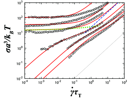
Figure 4: Experimental flow curves of a nearly hard sphere PMMA colloidal suspension, taken from Petekidis et al. pete , are shown using thermal units. The full lines are the fits using our additive model using $k_{B}T/\epsilon=10^{-8}$ and $\varphi_{\rm G}=0.575$; see also Table 1. For the first glass flow curve, we show the decomposition of the stress into its glass (dotted) and jamming (dashed) contributions. The thin dashed line represents the dilute limit. Clearly, the fluid to solid transition is a colloidal glass transition, with little influence from the jamming physics.

We have fitted the flow curves to the additive model. The fitting parameters are summarized in Table 1. Note that the particle softness $k_{B}T/\epsilon=10^{-8}$ used in our analysis is somewhat arbitrary, since this parameter does not strongly affect the flow curves in this thermal regime, as expected from the nearly hard sphere nature of the particles. As shown in Fig. 4, the transition between fluid and solid states is very well described by the glass rheology, and the fits indicate that the transition occurs for the volume fraction $\varphi_{\rm G}=0.575$. This is consistent with the analysis performed in the original paper pete . This value is also consistent with a mode-coupling analysis of the microscopic dynamics of colloidal hard spheres, for instance using light-scattering bill ; gio or microscopy techniques weeks . Thus our analysis confirms that the dynamic range probed in a typical rheology experiment is not broad enough for the crossover to activated dynamics at large density (which has been observed numerically tom2 and using other experimental approaches gio ) to become apparent.

Although it is clearly glass physics that controls the overall features of the flow curves, it is interesting to ask whether jamming physics also manifests itself. We argue that in Fig. 4 there are two distinct aspects where this is the case. First, we note that the yield stress reaches the value $\sigma^{\rm yield}/\sigma_{\rm T}\approx 10^{2}$ for the largest volume fraction, $\varphi=0.62$. This large value implies that the density is not very far from the jamming density so that the divergence in Eq. (19) starts to become relevant and a simplified expression for the yield stress, such as Eq. (18), would not account for the experimental data taken deep in the glass phase.

Accordingly, if the density is close enough to $\varphi_{\rm J}$, then the athermal Newtonian viscosity $\eta_{0}(\varphi)$ should also start to become large, as it is controlled by a similar diverging expression, see Eq. (17). From the above discussion of the model, see for instance Fig. 2, this viscosity is contributing to the flow curves at large Péclet number. This is demonstrated in Fig. 4 by the dashed line representing the jamming contribution to the total shear stress, $\sigma_{\rm J}\approx\eta_{0}(\varphi)\dot{\gamma}$. However, while our model predicts that $\eta_{0}$ grows rapidly when $\varphi\to\varphi_{\rm J}$, such a growth is not observed experimentally, and there are clear deviations between the fit and the data for the largest density in Fig. 4. This might indicate that the PMMA colloids cease to behave as nearly hard spheres at large densities and large Péclet numbers.

We suggest that it would be interesting to repeat such steady state rheological measurements with slightly larger PMMA particles so that large Péclet numbers and large densities are more easily studied. The crossover between glass and jamming rheology should then become more apparent and its features could be elucidated experimentally in this well-studied colloidal system.

III.3 Jamming physics: Aqueous foam

We now analyze the flow curves of aqueous foam reported by Herzhaft et al. foam . Foams are considered as prototypical materials displaying a jamming transition, because their are typically made of non-colloidal soft bubbles. It is worth mentionning that the harmonic sphere model considered numerically in Sec. II.1 was first devised to study the jamming rheology of wet foams durian .

The experimental system is composed of nitrogen bubbles dispersed in an aqueous polymer solution. Flow curve were measured at various densities. However, the particle size also changes with the density. We extracted the average particle diameter for each density from the reported particle size distributions. Note that the typical diameter is rather large at $27\,\mu{\rm m}$, with some size polydispersity. The reported solvent viscosity is $\eta_{s}=13$ mPa$\cdot$s. Using these values, we have estimated the thermal time scale and stress scale for each density. Typical values are $\tau_{\rm T}=5\cdot 10^{5}\,{\rm s}$ and $\sigma_{\rm T}=2\cdot 10^{-7}\,{\rm Pa}$, which are clearly outside the experimentally accessible windows for typical time and stress measurements. We represent the experimental flow curves using these thermal units in Fig. 5. As expected this produces large dimensionless numbers (such as $\dot{\gamma}\tau_{\rm T}\sim 10^{7}-10^{9}$). Clearly, these flow curves belong to the athermal sector, and should mainly be controlled by the jamming contribution to the shear stress.

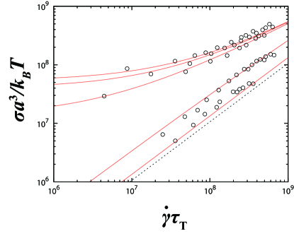
Figure 5: The experimental flow curves of aqueous foam in thermal units, after Herzhaft et al. foam . The red curves are fit by the additive model with $k_{B}T/\epsilon=2.10^{-11}$ and $\varphi_{\rm J}=0.55$; see also Table 1. The fluid to solid transition occurs in the jamming sector, with negligible influence from thermal fluctuations.

In the case of a bubble or droplet, we can estimate the particle softness using the surface tension $A$. The pressure inside a bubble is larger by $\Delta P=4A/a$ than on the outside, $\Delta P$ being the Laplace pressure. This pressure difference acts as a repulsive force between two overlapping particles. When the overlap length is $d$, the interface area between the ‘overlapping’ bubbles is given by $\pi a^{2}d/2$, and the repulsive force becomes $2\pi Aad$. Interpreting this force as the derivative of a pair interaction potential, we estimate the softness as $\epsilon=2\pi Aa^{2}$. This expression and the reported surface tension $A$ lead us to estimate the dimensionless particle softness for this system to be $k_{B}T/\epsilon=3\cdot 10^{-11}$, which is indeed very close to the athermal limit in which jamming physics should be observed.

We fitted the experimental flow curves to our model equation using this particle softness. The result and fitting parameters are shown in Fig. 5 and Table 1. The transition is well fitted as a jamming transition with $\varphi_{\rm J}=0.55$. Note that this value is much lower than the random close packing density usually quoted for spherical particles, $\varphi_{\rm J}\approx 0.64$. The reason of this deviation is not very clear. We can invoke the fact that the interaction between real bubbles is more complicated than in simple models of repulsive spheres, or the idea that additional microscopic dissipation channels exist in the real material, due for instance to some internal degrees of freedom of the bubbles. We note, however, that in other studies the jamming transition of a real foam was identified and located very close to the jamming transition occurring in simple harmonic sphere models, both at the level of static martin and rheological stjalmes properties.

III.4 Exploring the crossover: Oil-in-water emulsions

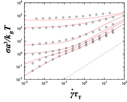
Figure 6: Experimental flow curves of oil-in-water emulsion in thermal units, after Mason et al. bibette . The red curves are fits to the additive model with $k_{B}T/\epsilon=3\cdot 10^{-7}$, $\varphi_{\rm G}=0.579$ and $\varphi_{\rm J}=0.62$; see also Table 1. While a glass transition is observed at low shear rates, the sharp increase of the yield stress in the glass phase is a signature of the jamming transition.

We next focus on the flow curves obtained for oil-in-water emulsions, reported by Mason et al. bibette . The system is composed of oil droplets stabilized with sodium dodecyl sulfate, which are dispersed in water. Although experiments with different particle diameters were performed bibette , we only analyze the results for droplet diameter $a=0.5\,\mu{\rm m}$ (with less than 10 % size dispersity), because the most complete set of flow curves were reported for this specific particle size bibette . Using the water viscosity value of $\eta_{s}=1$ mPa$\cdot$s, we estimate the thermal time and stress scales to be $\tau_{\rm T}=0.25\,{\rm s}$ and $\sigma_{\rm T}=3\cdot 10^{-2}\,{\rm Pa}$, respectively. These values are well within the measurable range and then we expect aspects of the glass transition to be relevant, although large Péclet numbers can certainly be accessed too. However, it is important to note that, in contrast to PMMA colloids as discussed in Sec. III.2, emulsions are made of soft droplets which can therefore easily be compressed above the jamming (or ‘random close packing’) density. This implies that aspects of the jamming transition are also potentially important for this system. The fact that features of both transitions are relevant for these emulsions is already apparent from the original experimental papers: the linear rheology of these systems was interpreted using the concepts of $\alpha$ and $\beta$ relaxations and power law scalings near the glass transition density $\varphi_{\rm G}$ inspired by mode-coupling theory mason , while the density dependence of the yield stress was fitted to a power law near the jamming density $\varphi_{\rm J}$ in a separate article bibette . Our additive model represents an ideal framework to unify and rationalize these findings.

The complex rheological features summarized above can be seen in Fig. 6, where the experimental flow curves are shown in thermal units. The system behaves as a Newtonian fluid at low enough density, $\varphi\leq 0.57$, and as a yield stress fluid for larger densities. However, the behaviour of the yield stress in the glass phase is clearly nontrivial, as it increases sharply with $\varphi$ in the range $\varphi\approx 0.60-0.62$ to reach large dimensionless values, $\sigma^{\rm yield}/\sigma_{\rm T}\approx 4\cdot 10^{2}$ for $\varphi=0.65$. This final shear stress value should belong to the athermal regime, possibly suggesting a crossover between the glass and jammed phases.

To confirm these qualitative conclusions, we fit the experimental flow curves using the additive rheological model. To this end, we first estimate the particle softness from the surface tension reported in the experimental article bibette , using the method outlined in the previous subsection for aqueous foams. We obtain $k_{B}T/\epsilon=3\cdot 10^{-7}$. Interestingly, this value is much larger than the one obtained for both foams and PMMA colloids, but remains at the lower end of the range of temperatures simulated in our numerical simulations letter ; see Fig. 1. We then fitted the experimental flow curves to the model equation using this softness value, and obtained the fits shown with lines in Fig. 6. The corresponding fitting parameters are listed in Table. 1. We obtain the glass and jamming transition densities at $\varphi_{\rm G}=0.579$ and $\varphi_{\rm J}=0.62$, these values being consistent with previous experimental analysis mason ; bibette . We emphasize that both the fluid to solid transition observed at low Péclet numbers, and the sharp increase with density of the yield stress are well fitted by our model. This allows us to conclude unambiguously that the transition which appears near $\varphi=0.58$ is a colloidal glass transition, while that the sharp stress increase at higher density near $\varphi\sim 0.62$ is a clear signature of the jamming transition. We stress that to obtain a quantitative description of these flow curves, it is absolutely necessary that both glass and jamming contributions to the shear stress are combined in a unified model as in Eq. (8). Therefore, the excellent fits in Fig. 6 provide strong experimental support for the additive model and theoretical analysis offered in the present work. As a direct physical corollary, we also conclude that the shear rheology of micron-size emulsions is quite complex, as the flow curves reveal all the features described by the most complex version of our additive rheological model.

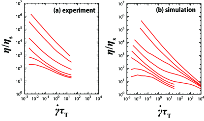
Figure 7: Viscosity vs. shear flow curves measured (a) experimentally for oil-in-water emulsions bibette and (b) numerically for harmonic spheres at $k_{B}T/\epsilon=10^{-6}$. We use similar dimensionless scales to emphasize the similarity between the two situations, suggesting that emulsions are an ideal experimental system to study the glass-jamming crossover.

As shown in Table 1, the parameters used to describe the emulsion data are very similar to the ones used to fit the flow curves of harmonic spheres in Fig. 1. This implies that the two sets of data should in fact be quantitatively very close. To show this more directly, we replot the flow curves for both these systems in a slightly different representation in Fig. 7, where the shear rate dependence of the effective viscosity, $\eta(\dot{\gamma})\equiv\sigma(\dot{\gamma})/\dot{\gamma}$, is shown. We make the experimental viscosity dimensionless using the solvent viscosity $\eta_{s}$, and combine Stokes’ law in Eq. (10) with Eq. (3) to obtain the bare viscosity $\eta_{s}=\xi/(3\pi a)$ in the numerics. The results in Fig. 7 are clearly very similar. This means that, somewhat surprisingly, modelling of real emulsions as harmonic spheres with overdamped Langevin dynamics is quantitatively very accurate. Our results also suggest that an interesting athermal Newtonian behavior characterized by the viscosity $\eta_{0}$ would appear experimentally if higher shear rates could be studied. (Note that, unusually, the range of shear rates studied is actually broader here in the numerical work than in the experiments). This second viscosity should be directly controlled by the jamming transition, and emulsions could thus be used to improve our understanding of its density dependence, which is usually studied using non-Brownian granular suspensions lindner ; boyer . We suggest that a more extensive rheological investigation of emulsions, perhaps by varying the droplet size in a more systematic manner to gradually access larger Péclet numbers, would be very interesting. We have found literature data for much larger particle diameters otsubo ; otsubo2 , but the density range covered in these flow curves was too limited to perform a detailed analysis of their evolution using our model.

Table 1: Summary of fitting parameters used in the paper. For emulsion, we used the same values of $Y_{\rm J}$ and $\beta_{\rm J}$ as in the original article bibette .

System	$p_{\rm G}$	$p_{\rm J}$	$h_{\rm G}$	$h_{\rm J}$	$\alpha_{\rm G}$	$\alpha_{\rm J}$	$\gamma_{\rm G}$	$\gamma_{\rm J}$	$Y_{\rm G}$	$Y_{\rm G}^{\prime}$	$Y_{\rm GJ}$	$Y_{\rm J}$	$\beta_{\rm G}$	$\beta_{\rm GJ}$	$\beta_{\rm J}$
Simulation letter	7	4	0.03	0.1	0.3	0.5	2.2	2.0	0.15	0.25	0.02	0.02	0.6	1.0	1.0
PMMA colloids pete	3	4	0.03	0.3	0.3	0.5	2.2	2.0	1.5	6.0	0.02	0.02	0.6	1.0	1.0
Foam foam	7	12	0.03	0.08	0.3	0.6	2.2	2.0	0.15	0.25	0.02	0.01	0.6	1.0	1.0
Emulsion bibette	7	0.5	0.03	0.06	0.3	0.5	2.2	2.0	0.25	0.65	0.02	0.016	0.6	1.0	2.0
PNIPAM carrier	7	1	0.03	0.07	0.5	0.4	2.2	2.0	12	30	1.5	0.03	0.6	1.0	1.0
PNIPAM yodh	30	1	0.2	0.005	0.5	0.4	2.2	2.0	15	500	3.5	3	0.6	1.0	1.0

III.5 PNIPAM microgels: Glass or jamming?

In this final experimental subsection, we analyze the steady state flow curves obtained for two independent sets of similar PNIPAM microgels. These particles are currently the focus of a large number of investigations microgelbook , for at least two reasons. First, these particles are made of microgels, and are therefore very soft. As such, they represent a new type of colloidal system, potentially very distinct from the more heavily studied hard sphere paradigm microgelnature . A second important feature is that PNIPAM microgels are highly sensitive to temperature, in the sense that a small temperature change induces a relatively large change of the particle size. This endows microgel suspensions with peculiar physical properties microgelbook .

We have analyzed two sets of flow curves obtained experimentally. One is reported by Carrier et al. carrier and was interpreted there in the framework of the mode-coupling theory extended to sheared fluids fuchs , thus implying the assumption that the fluid to solid transition in microgel suspensions is a colloidal glass transition. The second one is reported by Nordstrom et al. yodh . In this article, the flow curves are scaled using a procedure that was first employed in the context of the jamming transition of soft spheres olson , and the authors interpret the fluid to solid transition as the result of jamming. Our model, based as it is on a careful distinction between glass and jamming physics, is thus a natural tool to resolve the conflict between two opposing interpretations of the data.

Like for other systems, our first task is to replot the flow curves in dimensionless units, using the particle size and solvent viscosity to determine the relevant thermal units; see Fig. 8. In the first experiment carrier , the authors had reported their flow curves using similar thermal units. However, the particle radius was used as a microscopic length scale. To be consistent with the analysis performed elsewhere in the paper, we replotted the results using the particle diameter as the unit length. In the second experiment yodh , the results are reported in units of ${\rm Pa}$ and ${\rm s^{-1}}$ for shear stress and shear rate, respectively. The authors also reported the particle diameter as a function of temperature, and the corresponding packing fraction . Using these diameters and the reported solvent viscosity, $\eta_{s}=1\,{\rm mPa}\cdot{\rm s}$, we converted these flow curves to the dimensionless representation shown in Fig. 8. Once this rescaling is performed, it becomes evident that the experimental results obtained by the two research groups extend over a very similar range of shear stresses and shear rates. Thus the simple dimensional procedure indicates that the physics probed in these two experiments is the same. In particular, we notice immediately that the experiments are performed over a range of shear rates corresponding to relatively small Péclet numbers, down to $P_{\rm e}=10^{-4}$. This is because the particle size is small enough for thermal fluctuations to be relevant over the typical timescale of the experiments. Note that when converted into dimensionless units using the athermal timescale $\tau_{0}$, as done in Ref. yodh , the typical time scales extracted from the flow curves become unphysically large, $\tau/\tau_{0}\sim 10^{7}-10^{11}$, again indicating that the experimental data do not belong to the athermal jamming sector.

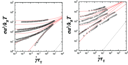
Figure 8: Experimental flow curves of PNIPAM microgels of (left) Carrier et al. carrier and (right) Nordstrom et al. yodh , using thermal units. The red curves are fit by the additive model with $k_{B}T/\epsilon=10^{-4}$ in both cases; see also Table 1. The corresponding glass transition densities are $\varphi_{\rm G}=0.68$ (left) and $\varphi_{\rm G}=0.638$ (right).

An independent confirmation of the relevance of thermal fluctuations for PNIPAM microgels is obtained from the linear viscoelastic experiments performed by Carrier et al. carrier . Their results show that the loss modulus $G^{\prime\prime}(\omega)$ becomes larger than the storage modulus $G^{\prime}(\omega)$ at low frequency. This indicates that spontaneous relaxation induced by thermal motion plays an important role in the rheology. Qualitatively similar results mason have been obtained, for instance, for the emulsion system discussed in Sec. III.4.

In order to fit the experimental data on PNIPAM microgels to our additive model, we have to estimate the particle softness $k_{B}T/\epsilon$. However, it is not obvious that the interaction between microgel particles can be approximated with a soft harmonic repulsion. Fortunately, a quantitative test of this assumption was performed in a detailed analysis of the vibrational properties of the amorphous solid phase of PNIPAM particles chen . For a similar system this study establishes the quality of the mapping and obtains $k_{B}T/\epsilon=2\cdot 10^{-5}$. A slightly larger value, near $k_{B}T/\epsilon=10^{-4}$, was later determined through a theoretical analysis of the mean-squared displacements of PNIPAM particles ikeda .

Using $k_{B}T/\epsilon=10^{-4}$ for the value of the particle softness, we then fitted both sets of flow curves to our additive model. The result of this procedure is shown in Fig. 8. The quality of the fits is similar to the one obtained within the mode-coupling theory framework carrier . As is clear also from the numerical flow curves obtained for a similar temperature in Fig. 1, jamming physics plays virtually no role in these fits, and the main control parameter to be adjusted is the glass transition density, which we estimate as $\varphi_{\rm G}=0.68$ and $\varphi_{\rm G}=0.638$ for the first carrier and second yodh set of experiments, respectively. Therefore, we conclude that the transition between a viscous fluid and a soft solid observed at low shear rate in the data of Fig. 8 is a colloidal glass transition, thus favoring the interpretation of Carrier et al. carrier over the one of Nordstrom et al. yodh .

We notice that another effect of the large particle softness is that the glass transition density does not correspond to the one of the hard sphere system discussed in Sec. III.2, but is considerably larger. This results from the fact that at finite temperatures microgel particles can overlap while hard spheres cannot, thereby shifting the glass transition density to larger values, as observed numerically tom ; tom2 and captured theoretically using a mode-coupling approach szamel . We emphasize that the quantitative similarity between the glass transition density of harmonic spheres and the jamming transition of hard sphere particles is then nothing but a numerical coincidence.

Another difference between hard and soft particles lies in the value of the typical yield stress scales observed in the experiments, see Fig. 8, which is somewhat larger for the soft microgel particles. To account for this feature, we had to use a larger value of the parameter $Y_{G}^{\prime}$ (see Table 1) which sets the scale of the yield stress in Eq. (21). We note that a similar change of numerical prefactor by about an order of magnitude was introduced (with no discussion) in the mode-coupling analysis of Carrier et al. carrier . We speculate that the effect could be due to the influence of polymeric internal degrees of freedom of the microgel particles.

While the microgel rheology analyzed in this subsection leads us to the conclusion that dense PNIPAM assemblies should be considered as thermal glasses rather than athermal jammed solids, we suggest that performing experiments with larger PNIPAM particles would be extremely rewarding, as this would produce an experimental system where large Péclet numbers could be studied with particles that are very soft. This would allow the jamming transition and rheology of soft particle systems to be studied experimentally martin ; xchen ; sessoms .

IV Summary and perspectives

In this paper, we described in detail the ‘additive’ rheological model first introduced in our numerical analysis of the interplay between glass and jamming rheologies letter , and we used the model to revisit published experimental data.

In our model, the stress contributions from thermal glass and athermal jamming physics are treated separately and we assume they can be linearly combined in a unified model. Because we want to describe the emergence of amorphous solids at large density for both colloidal and non-Brownian repulsive particles, the main control parameters for the formation of soft solids are therefore the particle packing fraction, $\varphi$, and the particle softness expressed in units of thermal energy, $k_{B}T/\epsilon$. From the analysis of numerical data obtained for harmonic spheres at both finite and zero temperatures, we developed simple functional forms for the flow curves $\sigma(\dot{\gamma})$ measured at a given state point, for the Newtonian viscosities $\eta_{T}$ and $\eta_{0}$ (in the fluid regimes), and for the yield stress $\sigma^{\rm yield}$ (in the solid phases).

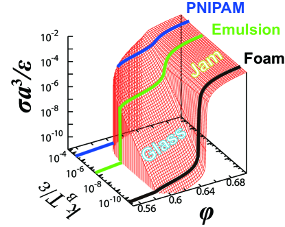
Figure 9: Three-dimensional ‘jamming phase diagram’ showing the yield stress surface as a function of the thermodynamic parameters temperatures and density, in a dimensionless representation (particle softness $k_{B}T/\epsilon$, volume fraction $\varphi$, and stress $\sigma a^{3}/\epsilon$). The three lines represent the location of the experimental systems discussed in Sec. III. Foams are mainly sensitive to jamming physics, emulsions display an interesting interplay between glass and jamming transitions, while PNIPAM microgels undergo a colloidal glass transition.

In particular, our additive model describes the emergence of solidity for soft repulsive systems as a function of temperature and volume fraction. As a result, we can use the yield stress fits shown in Fig. 3 to construct the three-dimensional ‘jamming phase diagram’ liunagel ; pica shown in Fig. 9, which represents the yield surface delimiting the solid and fluid phases for all values of the thermodynamic control parameters letter . This surface shows that the emergence of solidity at finite temperatures is always controlled by the colloidal glass transition, the $T=0$ point being the only situation where the jamming transition signals also the onset of solidity.

The line describing the PNIPAM microgel data in Fig. 9 corresponds to high temperatures (soft particles), and therefore the jamming transition does not influence the rheology of these microgel suspensions. When temperature is decreased, a clearer signature of the jamming transition is observed as a sharp increase of the yield stress with density. In this regime, the jamming transition appears as a change in the nature of the glass phase PZ ; hugo , but it does not control the emergence of solidity which still occurs at the glass transition. This description applies to emulsions, as shown in Fig. 9. Finally, when thermal effects become negligible, the thermal yield stress might become too small to be detected experimentally, and solidity genuinely emerges at the jamming transition. This is the case for foams in Fig. 9 for which the glass ‘wing’ has negligible effects. Note that PMMA colloidal suspensions would appear at nearly the same temperature/softness as foams in the jamming phase diagram of Fig. 9. However, with the particle size being much smaller than for foams, the yield stress emerging at the colloidal glass transition would easily be measured experimentally, and the measurements would stop as the jamming density is approached because the yield stress would seem to diverge there.

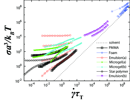
Figure 10: Superposition of experimental flow curves for different materials using thermal units. PMMA colloids with $a=0.36\,{\rm\mu m}$, after Petekidis et al. pete . Foam with $a=27\,{\rm\mu m}$, after Herzhaft et al. foam . Emulsion(a) with $a=0.5\,{\rm\mu m}$, after Mason et al. bibette . PNIPAM(a) with $a=0.2\,{\rm\mu m}$, after Carrier et al. yodh . PNIPAM(b) with $a=1.2\,{\rm\mu m}$, after Nordstrom et al. yodh . Star polymers with $a=0.07\,{\rm\mu m}$, after Koumakis et al. star . Emulsion(b) with $a=8\,{\rm\mu m}$, after Otsubo et al. otsubo .

As shown by the jamming phase diagram in Fig. 9, our analysis is useful in organizing the physics of different experimental systems. To confirm this, we have used our additive rheological model to analyze various experimental flow curves obtained for a variety of dense suspensions. The systems we focussed on were PMMA colloids pete , aqueous foam foam , oil-in-water emulsions bibette , and PNIPAM microgels carrier ; yodh . We have also gathered experimental data from other sources, in particular ultrasoft particles composed of star polymers star , and data for emulsions with larger droplet sizes otsubo , but for brevity the results of our analysis have not been presented in Sec. III.

We showed that all the above experimental results can be successfully analyzed using the additive model. It is instructive to replot all data in a single figure using the dimensional procedure adopted throughout this paper, i.e. expressing stress and time scales in thermal units $\sigma_{\rm T}$ and $\tau_{\rm T}$, see Eqs. (3, 5). These flow curves are collected in Fig. 10. In this representation, the flow curves for PMMA colloids, star polymers, PNIPAM microgels lie in the same sector, which corresponds to the thermal sector in our model; see Fig. 2. Therefore, the formation of amorphous solids in these systems stems from the physics of the colloidal glass transition. On the other hand, foams lie outside this regime and are controlled, accordingly, by the jamming transition. Interestingly, emulsions lie somewhat in between and so are influenced by both types of physics, as discussed in Sec. III.4. Note in particular that emulsions with larger droplet sizes, also shown in Fig. 10, could be useful systems to fill the gap between colloids and foams. While experimental studies of microgel particles have been interpreted from the point of view of the jamming transition yodh , our analysis shows that for these soft colloidal particles the physics of jamming has, in fact, only a negligible effect. A similar conclusion has recently been reached based on the analysis of the short-time vibrational dynamics in the amorphous phase ikeda .

Our conclusion that glass and jamming rheologies belong to different sectors and contribute linearly to the shear stress is directly supported by the numerical flow curves obtained for harmonic spheres, and by the analysis of the oil-in-water emulsions in Sec. III.4 which clearly showed the complex features also observed in the simulations. We mentioned that similar indications are also found for PMMA colloids, in particular at large Péclet number and larger density, while microgel suspensions appear less well suited for a detailed experimental investigations of the interplay between glass and jamming rheology. The data in Fig. 10 show that many current experimental systems are in fact too close to the thermal sector. Therefore, to fill the gap between small colloids and foams, measurements on sufficiently hard particles (PMMA colloids, emulsions) with particle sizes in the range $a=0.5-5\,\mu{\rm m}$ would appear ideally suited. We hope our work will stimulate experimental investigations in this direction.

- (1) R. G. Larson, The Structure and Rheology of Complex Fluids (Oxford University Press, New York, 1999).
- (2) P. Coussot, Rheometry of Pastes, Suspensions, and Granular Materials (Wiley, New York, 2005).
- (3) L. Berthier and G. Biroli, Rev. Mod. Phys. 83, 587 (2011).
- (4) A. J. Liu and S. R. Nagel, Annual Reviews of Cond. Mat. Phys. 1, 347 (2010).
- (5) P. N. Pusey and W. van Megen, Nature (London) 320, 340 (1986).
- (6) A. J. Liu and S. R. Nagel, Nature 396, 21 (1998).
- (7) Jamming and rheology, Eds.: A. J. Liu and S. R. Nagel (Taylor and Francis, New York, 2001).
- (8) C. S. O’Hern, S. A. Langer, A. J. Liu, and S. R. Nagel, Phys. Rev. Lett. 88, 075507 (2002).
- (9) M. van Hecke, J. Phys.: Condens. Matter 22 033101 (2010).
- (10) Dynamical heterogeneities in glasses, colloids and granular materials, Eds.: L. Berthier, G. Biroli, J.-P. Bouchaud, L. Cipelletti, and W. van Saarloos (Oxford University Press, Oxford, 2011).
- (11) R. Yamamoto and A. Onuki, Phys. Rev. E 58, 3515 (1998).
- (12) L. Berthier, J.-L. Barrat, and J. Kurchan Phys. Rev. E 61, 5464 (2000).
- (13) L. Berthier and J.-L. Barrat, J. Chem. Phys. 116, 6228 (2002).
- (14) M. Fuchs and M. E. Cates, Phys. Rev. Lett. 89, 248304 (2003).
- (15) M. Siebenbuerger, M. Fuchs, H. Winter, and M. Ballauff, J. Rheol 53, 707 (2009).
- (16) P. Olsson and S. Teitel, Phys. Rev. Lett. 99, 178001 (2007).
- (17) B. P. Tighe, E. Woldhuis, J. J. C. Remmers, W. van Saarloos, and M. van Hecke, Phys. Rev. Lett. 105, 088303 (2010).
- (18) P. Olsson and S. Teitel, Phys. Rev. Lett. 109, 108001 (2012).
- (19) E. Lerner, G. Düring, and M. Wyart, Proc. Natl. Acad. Sci. USA 109, 4798 (2012).
- (20) P. Guan, M. Chen, and T. Egami, Phys. Rev. Lett. 104, 205701 (2010).
- (21) K. N. Nordstrom, E. Verneuil, P. E. Arratia, A. Basu, Z. Zhang, A. G. Yodh, J. P. Gollub, and D. J. Durian, Phys. Rev. Lett. 105, 175701 (2010).
- (22) A. Ikeda, L. Berthier, and P. Sollich, Phys. Rev. Lett. 109, 018301 (2012).
- (23) L. Berthier and T. A. Witten, EPL 86, 10001 (2009).
- (24) D. J. Durian, Phys. Rev. Lett. 75, 4780 (1995); Phys. Rev. E 55, 1739 (1997).
- (25) M. Allen and D. Tildesley, Computer Simulation of Liquids (Oxford University Press, Oxford, 1987).
- (26) P. Olsson and S. Teitel, arxiv:1211.2839.
- (27) T. Voigtmann, Eur. Phys. J. E 34, 106 (2011).
- (28) Z. Cheng, J. Zhu, P. M. Chaikin, S. E. Phan, and W. B. Russel, Phys. Rev. E 65, 041405 (2002).
- (29) W. van Megen, T. C. Mortensen, S. R. Williams, and J. Muller, Phys. Rev. E 58, 6073 (1998).
- (30) G. Brambilla, D. El Masri, M. Pierno, L. Berthier, L. Cipelletti, G. Petekidis, and A. B. Schofield, Phys. Rev. Lett. 102, 085703 (2009).
- (31) W. Götze, Complex Dynamics of Glass-Forming Liquids: A Mode-Coupling Theory (Oxford University Press, Oxford, 2008).
- (32) L. Berthier and T. A. Witten, Phys. Rev. E 80, 021502 (2009).
- (33) C. Bonnoit, T. Darnige, E. Clement, and A. Lindner, J. Rheol. 54, 65 (2010).
- (34) F. Boyer, E. Guazzelli, and O. Pouliquen, Phys. Rev. Lett. 107, 188301 (2011).
- (35) A. Donev, S. Torquato, F. H. Stillinger, and R. Connelly, Phys. Rev. E 70, 043301 (2004).
- (36) P. Chaudhuri, L. Berthier, and S. Sastry, Phys. Rev. Lett. 104, 165701 (2010).
- (37) J. Mewis and N. J. Wagner, Colloidal suspension rheology (Cambridge University Press, Cambridge, 2012).
- (38) M. H. Cohen and D. Turnbull, J. Chem. Phys. 31, 1164 (1959).
- (39) Z. W. Salsburg and W. W. Wood, J. Chem. Phys. 37, 798 (1962).
- (40) L. Berthier, H. Jacquin, and F. Zamponi, Phys. Rev. E 84, 051103 (2011).
- (41) G. Petekidis, D. Vlassopoulos, and P. N. Pusey, J. Phys.: Condens. Matter 16, S3955 (2004).
- (42) J. P. Hansen and I. R. McDonald, Theory of Simple Liquids (Elsevier, Amsterdam, 1986).
- (43) E. Weeks, J. C. Crocker, A. C. Levitt, A. Schofield, and D. A. Weitz, Science 287, 627 (2000).
- (44) B. Hertzhaft, S. Kakadjian, and M. Moan, Colloids Surf. A 263, 153 (2005).
- (45) G. Katgert and M. van Hecke, EPL 92, 34002 (2010).
- (46) A. Saint-Jalmes and D. J. Durian, J. Rheol. 43, 1411 (1999).
- (47) T. G. Mason, J. Bibette, D. A. Weitz, J. Colloid Interface Sci. 179, 439 (1996).
- (48) T. G. Mason and D. A. Weitz, Phys. Rev. Lett. 75, 2770 (1995).
- (49) Y. Otsubo and R. K. Prud’homme, Rheol. Acta 33, 29 (1994).
- (50) Y. Otsubo and R. K. Prud’homme, J. Soc. Rheol. Japan 20, 125 (1992).
- (51) Microgel suspensions, Eqs.: A. Fernandez-Nieves, H. Wyss, J. Mattsson, D. A. Weitz (Wiley, Weiheim, 2011).
- (52) J. Mattsson, H. M. Wyss, A. Fernandez-Nieves, K. Miyazaki, Z. Hu, D. R. Reichman, and D. A. Weitz, Nature 462, 83 (2009).
- (53) V. Carrier and G. Petekidis, J. Rheol. 53, 245 (2009).
- (54) K. Chen, W. G. Ellenbroek, Z. Zhang, D. T. N. Chen, P. J. Yunker, C. Brito, O. Dauchot, S. Henkes, W. van Saarloos, A. J. Liu, and A. G. Yodh, Phys. Rev. Lett. 105, 025501 (2010).
- (55) A. Ikeda, L. Berthier, and G. Biroli J. Chem. Phys. 138, 12A507 (2013).
- (56) L. Berthier, E. Flenner, H. Jacquin, and G. Szamel, Phys. Rev. E 81, 031505 (2010).
- (57) X. Cheng, Phys. Rev. E 81, 031301 (2010).
- (58) D. A. Sessoms, I. Bischofberger, L. Cipelletti, and V. Trappe, Philos. Trans. R. Soc. London, Ser. A 367, 5013 (2009).
- (59) M. Pica Ciamarra, M. Nicodemi and A. Coniglio, Soft Matter 6, 2871 (2010).
- (60) G. Parisi and F. Zamponi, Rev. Mod. Phys. 82, 789 (2010).
- (61) H. Jacquin, L. Berthier, and F. Zamponi, Phys. Rev. Lett. 106, 135702 (2011).
- (62) N. Koumakis, A. Pamvouxoglou, A. Poulos, and G. Petekidis, Soft Matter 8, 4271 (2012).