Anisotropic finite elements with high aspect ratio for an Asymptotic Preserving method for highly anisotropic elliptic equations

Abstract

The concern of this work is the generalization of an Asymptotic Preserving method for the highly anisotropic elliptic equations presented in [14]. The limitations of the method introduced there in are omitted by the introduction of a stabilization term in the Asymptotic Reformulation. Furthermore, anisotropic error indicators and mesh adaptation algorithms are proposed and tested allowing to reduce considerably the number of mesh points required to achieve prescribed precision. Reported meshes have maximum aspect ratio greater than 500.

1 Introduction

Anisotropic problems are common in mathematical modeling of physical problems. They appear in various fields of application, such as flows in porous media [4, 17], semiconductor modeling [21], quasi-neutral plasma simulations [11], image processing [28, 29], atmospheric or oceanic flows [27] and so on, the list being not exhaustive. The direct motivation of this work is related to numerical simulations of strongly magnetized plasma such as internal fusion plasma of tokamak [5, 13], atmospheric plasma [19, 20] or plasma thrusters [1]. In this context a strong magnetic field is defining the anisotropy direction. Fast rotation of charged particles around magnetic field lines is causing a large number of collisions in the plane perpendicular to the magnetic field. On the other hand the motion in the direction of the field is rather undisturbed. In consequence the particle mobility depends on the direction and may differ by several orders of magnitude. Anisotropy ratio $1/\varepsilon$ can be as high as $10^{10}$.

The main difficulty associated with these anisotropic problems is that they are singular in the limit $\varepsilon\rightarrow 0$. On the discrete level this is manifested by very bad conditioning of linear systems obtained by a direct discretization of the problem for $\varepsilon\ll 1$. In this paper we propose an approach based on the Asymptotic Preserving reformulation introduced initially by Shi Jin in [18]. Our approach is an extension of the method proposed in a previous paper [14] to the case of more general anisotropy field structure (such as closed field lines).

The model problem we are interested in, reads

$$\left\{\begin{array}[]{ll}-\nabla\cdot\mathbb{A}_{\varepsilon}\nabla u^{\varepsilon}=f&\text{ in }\Omega,\\[8.53581pt] n\cdot\mathbb{A}_{\varepsilon}\nabla u^{\varepsilon}=0&\text{ on }\Gamma_{N}\,,\\[8.53581pt] u^{\varepsilon}=0&\text{ on }\Gamma_{D}\,,\end{array}\right.$$ (4)

where $\Omega\subset\mathbb{R}^{2}$ is a bounded domain with boundary $\partial\Omega=\Gamma_{D}\cup\Gamma_{N}$ and outward normal $n$. The direction of the anisotropy is given by a vector field $B$, where we suppose $\text{div}B=0$ and $B\neq 0$. The direction of $B$ shall be denoted by the unit vector field $b=B/|B|$. The domain boundary is decomposed into $\Gamma_{D}:=\{x\in\partial\Omega\ |\ b(x)\cdot n=0\}$ and $\Gamma_{N}:=\partial\Omega\backslash\Gamma_{D}$. The anisotropic diffusion matrix is then given by

$$\mathbb{A}_{\varepsilon}=\frac{1}{\varepsilon}A_{\parallel}b\otimes b+(Id-b\otimes b)A_{\perp}(Id-b\otimes b)\,.$$ (5)

The scalar field $A_{\parallel}>0$ and the symmetric positive definite matrix field $A_{\perp}$ are of order one while the parameter $0<\varepsilon<1$ can be very small, provoking thus the high anisotropy of the problem. The system becomes ill posed if we consider the formal limit $\varepsilon\rightarrow 0$. It is thus very ill conditioned for $\varepsilon\ll 1$.

This problem has been studied before in the Asymptotic Preserving context. A special case of anisotropy direction aligned with one of the coordinate axis was addressed in [12]. A generalization of this approach was presented in [6], where the problem with curvilinear anisotropy field was reduced to one with the anisotropy direction aligned with the coordinate system by a change of variables. Another work [10] proposed a different generalization based rather on the introduction of Lagrange multipliers. This resulted in a considerably bigger linear system but allowed to avoid a necessity of change of variables which could be troublesome for time dependent anisotropy direction. Finally, a different method presented in [14] allowed to reduce considerably computational cost without any adaptation of the coordinate system. All those methods shared the same drawback: they didn’t allow more complex geometries such as the presence of closed field lines.

In this paper we introduce yet another Asymptotic Preserving scheme, improving the idea presented in [14] and removing the restrictions on the anisotropy direction by a simple penalty stabilization technique. Furthermore, the anisotropic error indicator is presented and the mesh adaptation algorithm developed in order to optimize the number of mesh points required to obtain a prescribed error.

The outline of the paper is following. Section 2 contains a definition of the problem and introduces the Asymptotic Preserving reformulation. Section 3 describes an anisotropic error indicator and mesh adaptation algorithm. They are both tested and the numerical results are provided.

2 Problem definition

We consider a two dimensional anisotropic problem, given on a regular, bounded domain $\Omega\subset\mathbb{R}^{2}$, with boundary $\partial\Omega$. The direction of the anisotropy is defined by the vector field $b(x)$, which satisfies the following hypothesis

Hypothesis A The field $b(x)$ is derived from a vector field $B(x)=|B(x)|\,b(x)$, satisfying $div\,\,B(x)=0$ and $|b(x)|=1$ for all $x\in\Omega$. Moreover, we suppose that $b\in(C^{\infty}(\Omega))^{d}$.

Given this vector field $b$, one can decompose now vectors $v\in\mathbb{R}^{2}$, gradients $\nabla\phi$, with $\phi(x)$ a scalar function, and divergences $\nabla\cdot v$, with $v(x)$ a vector field, into a part parallel to the anisotropy direction and a part perpendicular to it. These parts are defined as follows :

$$\begin{array}[]{llll}\displaystyle v_{||}:=(v\cdot b)b\,,&\displaystyle v_{\perp}:=(Id-b\otimes b)v\,,&\textrm{such that}&\displaystyle v=v_{||}+v_{\perp}\,,\\[8.53581pt] \displaystyle\nabla_{||}\phi:=(b\cdot\nabla\phi)b\,,&\displaystyle\nabla_{\perp}\phi:=(Id-b\otimes b)\nabla\phi\,,&\textrm{such that}&\displaystyle\nabla\phi=\nabla_{||}\phi+\nabla_{\perp}\phi\,,\\[8.53581pt] \displaystyle\nabla_{||}\cdot v:=\nabla\cdot v_{||}\,,&\displaystyle\nabla_{\perp}\cdot v:=\nabla\cdot v_{\perp}\,,&\textrm{such that}&\displaystyle\nabla\cdot v=\nabla_{||}\cdot v+\nabla_{\perp}\cdot v\,,\end{array}$$ (6)

where we denoted by $\otimes$ the vector tensor product. With these notations we can now introduce the mathematical problem, the so-called Singular Perturbation problem, whose numerical resolution is the main concern of this paper.

2.1 The Singular Perturbation problem (P-model)

The objective of this paper is to introduce an efficient scheme for the precise ($\varepsilon$-independent) resolution of the following Singular Perturbation problem

$$(P)\,\,\,\left\{\begin{array}[]{ll}-{1\over\varepsilon}\nabla_{\parallel}\cdot\left(A_{\parallel}\nabla_{\parallel}\phi^{\varepsilon}\right)-\nabla_{\perp}\cdot\left(A_{\perp}\nabla_{\perp}\phi^{\varepsilon}\right)=f&\text{ in }\Omega,\\[8.53581pt] {1\over\varepsilon}n_{\parallel}\cdot\left(A_{\parallel}\nabla_{\parallel}\phi^{\varepsilon}\right)+n_{\perp}\cdot\left(A_{\perp}\nabla_{\perp}\phi^{\varepsilon}\right)=0&\text{ on }\partial\Omega_{in}\cup\partial\Omega_{out},\\[8.53581pt] \phi^{\varepsilon}=0&\text{ on }\partial\Omega_{D}\,,\end{array}\right.$$ (10)

where $n$ is the outward normal to $\Omega$ and the boundaries are defined by

$$\partial\Omega_{D}=\{x\in\partial\Omega\ |\ b(x)\cdot n=0\},$$ (11)

$$\partial\Omega_{in}=\{x\in\partial\Omega\ |\ b(x)\cdot n<0\},$$ (12)

$$\partial\Omega_{out}=\{x\in\partial\Omega\ |\ b(x)\cdot n>0\}.$$ (13)

The parameter $0<\varepsilon<1$ can be very small and is responsible for the high anisotropy of the problem. We shall assume in the rest of this paper the following hypothesis on the diffusion and source terms

Hypothesis B Let $f\in L^{2}(\Omega)$ and $\overset{\circ}{\partial\Omega_{D}}\neq\varnothing$. Furthermore, the diffusion coefficients $A_{\parallel}\in L^{\infty}(\Omega)$ and $A_{\perp}\in\mathbb{M}_{d\times d}(L^{\infty}(\Omega))$ are supposed to satisfy

$$0<A_{0}\leq A_{\parallel}(x)\leq A_{1}\,,\quad\textrm{f.a.a}\,\,\,x\in\Omega,$$ (14)

$$A_{\perp}(x)b(x)=A_{\perp}^{t}(x)b(x)=0\,,\quad\textrm{f.a.a}\,\,\,x\in\Omega,$$ (15)

$$A_{0}||v||^{2}\leq v^{t}A_{\perp}(x)v\leq A_{1}||v||^{2}\,,\quad\forall v\in\mathbb{R}^{d}\,\,\,\text{with}\,\,\,v\cdot b(x)=0\,\,\,\text{and}\,\,\,\textrm{f.a.a}\,\,\,x\in\Omega.$$ (16)

As we conceive to use the finite element method for the numerical resolution of the P-problem, let us put (10) under variational form. For this let $\mathcal{V}$ be the Hilbert space

$$\mathcal{V}:=\{\phi\in H^{1}(\Omega)\,\,/\,\,\phi_{|\partial\Omega_{D}}=0\}\,,\quad(\phi,\psi)_{\mathcal{V}}:=(\nabla_{\parallel}\phi,\nabla_{\parallel}\psi)_{L^{2}}+\varepsilon(\nabla_{\perp}\phi,\nabla_{\perp}\psi)_{L^{2}}\,.$$

We are searching thus for $\phi^{\varepsilon}\in\mathcal{V}$, solution of

$$a_{\parallel}(\phi^{\varepsilon},\psi)+\varepsilon a_{\perp}(\phi^{\varepsilon},\psi)=\varepsilon(f,\psi)\,,\quad\forall\psi\in\mathcal{V}\,,$$ (17)

where $(\cdot,\cdot)$ stands for the standard $L^{2}$ scalar product and the continuous, bilinear forms $a_{\parallel}:\mathcal{V}\times\mathcal{V}\rightarrow\mathbb{R}$ and $a_{\perp}:\mathcal{V}\times\mathcal{V}\rightarrow\mathbb{R}$ are given by

$$\begin{array}[]{lll}\displaystyle a_{\parallel}(\phi,\psi)&:=&\displaystyle\int_{\Omega}A_{||}\nabla_{||}\phi\cdot\nabla_{||}\psi\,dx\,,\quad a_{\perp}(\phi,\psi):=\displaystyle\int_{\Omega}(A_{\perp}\nabla_{\perp}\phi)\cdot\nabla_{\perp}\psi\,dx\,.\end{array}$$ (19)

Thanks to Hypothesis B and the Lax-Milgram theorem, the problem (10) admits a unique solution $\phi^{\varepsilon}\in\mathcal{V}$ for all fixed $\varepsilon>0$. However, the numerical resolution of (10) is very inadequate for $\varepsilon\ll 1$. When $\varepsilon$ tends to zero, the problem reduces to

$$\left\{\begin{array}[]{ll}\displaystyle-\nabla_{\parallel}\cdot\left(A_{\parallel}\nabla_{\parallel}\phi\right)=0&\text{ in }\Omega,\\[8.53581pt] \displaystyle n_{\parallel}\cdot\left(A_{\parallel}\nabla_{\parallel}\phi\right)=0&\text{ on }\partial\Omega_{in}\cup\partial\Omega_{out},\\[8.53581pt] \displaystyle\phi^{0}=0&\text{ on }\partial\Omega_{D}.\end{array}\right.$$ (23)

This is an ill-posed problem as it has an infinite number of solutions $\phi\in\mathcal{G}$, where

$$\mathcal{G}=\{\phi\in\mathcal{V}\ |\ \nabla_{\parallel}\phi=0\}\,,$$ (24)

is the Hilbert space of functions, which are constant along the field lines of $b$. On the discrete level this is manifested by a very bad conditioning of the system for small values of $\varepsilon$. However, as shown in [10], the solution $\phi^{\varepsilon}\in\mathcal{V}$ converges to $\phi^{0}\in\mathcal{G}$, a unique solution of

$$(L)\,\,\,\int_{\Omega}A_{\perp}\nabla_{\perp}\phi^{0}\cdot\nabla_{\perp}\psi\,dx=\int_{\Omega}f\psi\,dx\;\;,\;\;\forall\psi\in\mathcal{G}\,.$$ (25)

2.2 The Asymptotic Preserving approach (AP-model)

Let us introduce a so called AP-formulation, which is a reformulation of the Singular Perturbation problem (10), permitting a “continuous” transition from the (P)-problem (10) to the (L)-problem (25), as $\varepsilon\rightarrow 0$. The AP-formulation was introduced and is a subject of more detailed analysis in a separate publication [14]. We will shortly recall the results of the previous studies. For this, each function shall be decomposed into two parts: constant part along the anisotropy direction and a part containing fluctuations. The constant part converges to the limit solution and the fluctuating to $0$ as $\varepsilon\rightarrow 0$ (see also [14]).

Let us introduce the following Hilbert space:

$$\mathcal{A}:=\{q\in L^{2}(\Omega)\ /\nabla_{\parallel}q\in L^{2}(\Omega)\text{ and }q|_{\partial\Omega_{in}}=0\}$$ (26)

$$(q,w)_{\mathcal{A}}=(\nabla_{\parallel}q,\nabla_{\parallel}w)\;\;,\;\;\forall q,w\in\mathcal{A}.$$ (27)

Let $\phi^{\varepsilon}$ be a solution to the Singular Perturbation problem (10) and set $\phi^{\varepsilon}=p^{\varepsilon}+\varepsilon q^{\varepsilon}$ with $p^{\varepsilon}\in\mathcal{G}$ and $q^{\varepsilon}\in\mathcal{A}$. This decomposition is unique and we observe

$$\left\{\begin{array}[]{ll}a_{\perp}(p^{\varepsilon},v)+\varepsilon a_{\perp}(q^{\varepsilon},v)+a_{\parallel}(q^{\varepsilon},v)=(f,v)&\forall v\in\mathcal{V}\,,\\[8.53581pt] a_{\parallel}(p^{\varepsilon},w)=0&\forall w\in\mathcal{A}\,,\end{array}\right.$$ (30)

or equivalently

$$(AP)\,\,\,\left\{\begin{array}[]{ll}a(\phi^{\varepsilon},v)+(1-\varepsilon)a_{\parallel}(q^{\varepsilon},v)=(f,v)&\forall v\in\mathcal{V}\,,\\[8.53581pt] a_{\parallel}(\phi^{\varepsilon},w)=\varepsilon a_{\parallel}(q^{\varepsilon},w)&\forall w\in\mathcal{A}\,,\end{array}\right.$$ (33)

with the bilinear form $a(v,w)$ defined as

$$a(v,w)=\int_{\Omega}\mathbb{A}\nabla v\cdot\nabla w.$$ (34)

The matrix $\mathbb{A}$ is given by

$$\mathbb{A}=A_{\parallel}b\otimes b+(Id-b\otimes b)A_{\perp}(Id-b\otimes b),$$ (35)

and is $\varepsilon$ independent, $\mathbb{A}=\mathbb{A}_{1}$.

The above formulation is the Asymptotic Preserving reformulation based on the Micro Macro decomposition.

2.3 The stabilized Asymptotic Preserving approach (AP-model)

The Asymptotic Preserving approach presented above has some limitations originating in the choice of the vector space $\mathcal{A}$. Note that in the previous paper the uniqueness of $q^{\varepsilon}$ was ensured by setting $q^{\varepsilon}$ to $0$ on the $\Gamma_{in}$ boundary under hypothesis that every field line of $b$ has its beginning on $\Gamma_{in}$ and an end on $\Gamma_{out}$. In other words, more complex geometries, like for example closed field lines are not permitted. In this paper we propose a new way of providing the uniqueness of $q^{\varepsilon}$ which overcomes the limitations of our previous method. The idea is based on the penalty stabilization method introduced in [8] for the Stokes problem.

Let us propose a new Asymptotic Preserving method: find $(\phi^{\varepsilon},q^{\varepsilon})\in\mathcal{V}\times\mathcal{V}$ such that

$$(APS)\,\,\,\left\{\begin{array}[]{ll}a(\phi^{\varepsilon},v)+(1-\varepsilon)a_{\parallel}(q^{\varepsilon},v)=(f,v)&\forall v\in\mathcal{V}\,,\\[8.53581pt] a_{\parallel}(\phi^{\varepsilon},w)=\varepsilon a_{\parallel}(q^{\varepsilon},w)+\sum_{K\in\tau_{h}}h_{K}^{2}\int_{K}\mathbb{A}\nabla q^{\varepsilon}\cdot\nabla w&\forall w\in\mathcal{V}\,,\end{array}\right.$$ (38)

where $h_{K}$ denotes the size of the element $K$. Note that now, instead of seeking $q^{\varepsilon}\in\mathcal{A}$ we are looking for $q^{\varepsilon}\in\mathcal{V}$. Existence and uniqueness of the above problem can be easily proved by the Lax-Milgram theorem.

3 Numerical method

This section concerns the discretization of the Asymptotic Preserving formulation (38), based on a finite element method. The anisotropic error indicator is introduced and the obtained numerical results are studied.

Let us denote by $\mathcal{V}_{h}\subset\mathcal{V}$ and $\mathcal{A}_{h}\subset\mathcal{A}$ the finite dimensional approximation spaces, constructed by means of $P_{1}$ finite elements. We are thus looking for a discrete solution $(\phi^{\varepsilon}_{h},\;q^{\varepsilon}_{h})\in\mathcal{V}_{h}\times\mathcal{A}_{h}$ of the following system

$$(APS)_{h}\,\,\,\left\{\begin{array}[]{ll}a(\phi^{\varepsilon}_{h},v_{h})+(1-\varepsilon)a_{\parallel}(q^{\varepsilon}_{h},v_{h})=(f_{h},v_{h})&\forall v_{h}\in\mathcal{V}_{h}\,,\\[8.53581pt] a_{\parallel}(\phi^{\varepsilon}_{h},w_{h})=\varepsilon a_{\parallel}(q_{h}^{\varepsilon},w_{h})+\sum_{K\in\tau_{h}}h_{K}^{2}\int_{K}\mathbb{A}\nabla q^{\varepsilon}_{h}\cdot\nabla w_{h}&\forall w_{h}\in\mathcal{V}_{h}\,.\end{array}\right.$$ (41)

3.1 Adaptive finite elements with large aspect ratio

We now propose an adaptive finite element algorithm. The goal is to build successive triangulations with large aspect ratio such that the relative estimated error of the function $\phi^{\varepsilon}=p^{\varepsilon}+\varepsilon q^{\varepsilon}$ in the $H^{1}(\Omega)$ norm is close to a preset tolerance $TOL$. For this purpose, we introduce an error indicator which requires some further notations. This error indicator measures the error of the numerical solution $\phi^{\varepsilon}$ in the directions of maximum and minimum stretching of the triangle. The goal of the adaptive algorithm is then to equidistribute the error indicator in the directions of maximum and minimum stretching, and to align the directions of maximum and minimum stretching with the directions of maximum and minimum error. We refer to [24, 23, 9, 15, 16] for theoretical justifications.

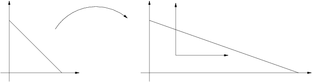
Figure 1: A simple example of transformation from reference triangle $\hat{K}$ to generic triangle $K$.

For any triangle $K$ of the mesh, let $T_{K}:\hat{K}\to K$ be the affine transformation which maps the reference triangle $\hat{K}$ into $K$. Let $M_{K}$ be the Jacobian of $T_{K}$ that is

$$\mathbf{x}=T_{K}(\hat{\mathbf{x}})=M_{K}\hat{\mathbf{x}}+\mathbf{t}_{K}.$$

Since $M_{K}$ is invertible, it admits a singular value decomposition $M_{K}=R_{K}^{T}\Lambda_{K}P_{K}$, where $R_{K}$ and $P_{K}$ are orthogonal and where $\Lambda_{K}$ is diagonal with positive entries. In the following we set

$$\Lambda_{K}=\begin{pmatrix}\lambda_{1,K}&0\\ 0&\lambda_{2,K}\end{pmatrix}\qquad\text{and}\qquad R_{K}=\begin{pmatrix}\mathbf{r}_{1,K}^{T}\\ \mathbf{r}_{2,K}^{T}\end{pmatrix},$$

with the choice $\lambda_{1,K}\geq\lambda_{2,K}$. A simple example of such a transformation is $x_{1}=H\hat{x}_{1}$, $x_{2}=h\hat{x}_{2}$, with $H\geq h$, thus

$$M_{K}=\begin{pmatrix}H&0\\ 0&h\end{pmatrix}\quad\lambda_{1,K}=H,\quad\lambda_{2,K}=h,\quad\mathbf{r}_{1,K}=\begin{pmatrix}1\\ 0\end{pmatrix},\quad\mathbf{r}_{2,K}=\begin{pmatrix}0\\ 1\end{pmatrix},$$

see Figure 1. In other words $\mathbf{r}_{1,K}$ and $\mathbf{r}_{2,K}$ are the directions of maximum and minimum stretching, while $\lambda_{1,K}$ and $\lambda_{2,K}$ measure the amplitude of stretching.

Let $I_{h}:H^{1}_{0}(\Omega)\rightarrow\mathcal{V}_{h}$ be a Clément or Scott-Zhang like interpolation operator. We now recall some interpolation results due to [15, 16, 22].

Proposition 1.

There is a constant $C=C(\hat{K})$ such that for all $v\in H^{1}(\Omega)$, for all $K\in\tau_{h}$, for all edges $e$ of $K$, we have

$$||v-I_{h}v||_{L^{2}(\Omega)}\leq C\left(\lambda_{1,K}^{2}(\mathbf{r}_{1,K}G_{K}(v)\mathbf{r}_{1,K})+\lambda_{2,K}^{2}(\mathbf{r}_{2,K}G_{K}(v)\mathbf{r}_{2,K})\right)^{1/2},$$ (42)

$$||v-I_{h}v||_{L^{2}(e)}\leq Ch_{K}^{1/2}\left(\frac{\lambda_{1,K}}{\lambda_{2,K}}(\mathbf{r}_{1,K}G_{K}(v)\mathbf{r}_{1,K})+\frac{\lambda_{2,K}}{\lambda_{1,K}}(\mathbf{r}_{2,K}G_{K}(v)\mathbf{r}_{2,K})\right)^{1/2},$$ (43)

$$||\nabla(v-I_{h}v)||_{L^{2}(K)}\leq C\left(\frac{\lambda_{1,K}^{2}}{\lambda_{2,K}^{2}}(\mathbf{r}_{1,K}G_{K}(v)\mathbf{r}_{1,K})+(\mathbf{r}_{2,K}G_{K}(v)\mathbf{r}_{2,K})\right)^{1/2}.$$ (44)

Here $h_{k}=\text{diam }K$, $\lambda_{i,K}$ and $\mathbf{r}_{i,K}$ are given by (3.1), and $G_{K}(v)$ denotes the $2\times 2$ matrix defined as

$$G_{K}(v)=\begin{pmatrix}\displaystyle{\int_{K}\left(\frac{\partial v}{\partial x_{1}}\right)^{2}dx}&\displaystyle{\int_{K}\left(\frac{\partial v}{\partial x_{1}}\right)\left(\frac{\partial v}{\partial x_{2}}\right)dx}\\ \displaystyle{\int_{K}\left(\frac{\partial v}{\partial x_{1}}\right)\left(\frac{\partial v}{\partial x_{2}}\right)dx}&\displaystyle{\int_{K}\left(\frac{\partial v}{\partial x_{2}}\right)^{2}dx}\end{pmatrix}.$$ (45)

Proof.

The first estimate is in Proposition 3.1 of [15], the second estimate is in Proposition 2.2 of [16], the third estimate is in Proposition 2.5 of [22]. ∎

The results of Proposition 1 are now used to derive an anisotropic error indicator for the Asymptotic Preserving reformulation. The error is first related to the equation residual. The Clément interpolant is introduced. Then the anisotropic interpolation results are used. Finally, a Zienkiewicz-Zhu error estimator is used to approach the error gradient.

Let $e=\phi^{\varepsilon}-\phi^{\varepsilon}_{h}$ and $e_{q}=q^{\varepsilon}-q^{\varepsilon}_{h}$. The following error estimate for the Asymptotic Preserving reformulation (33) holds.

Proposition 2.

There exist a constant $C$ depending only on the interpolation constants from Proposition 1 and not on the mesh size nor aspect ratio such that

$$\int_{\Omega}\mathbb{A}\nabla e\cdot\nabla e+(1-\varepsilon)\varepsilon\int_{\Omega}A_{\parallel}\nabla_{\parallel}e_{q}\cdot\nabla_{\parallel}e_{q}+(1-\varepsilon)\sum_{K\in\tau_{h}}h_{K}^{2}\int_{K}\mathbb{A}\nabla e_{q}\cdot\nabla e_{q}\leq\\ \ C\sum_{K\in\tau_{h}}\Bigg{(}||f+\nabla\cdot(\mathbb{A}\nabla\phi^{\varepsilon}_{h})+(1-\varepsilon)\nabla_{\parallel}\cdot(A_{\parallel}\nabla_{\parallel}q^{\varepsilon}_{h})||_{L^{2}(K)}\\ +\frac{1}{2\lambda_{2,K}^{1/2}}||[\mathbb{A}\nabla\phi^{\varepsilon}_{h}\cdot n]||_{L^{2}(\partial K)}+\frac{1-\varepsilon}{2\lambda_{2,K}^{1/2}}||[A_{\parallel}\nabla_{\parallel}q^{\varepsilon}_{h}\cdot n]||_{L^{2}(\partial K)}\Bigg{)}\\ \times\left(\lambda_{1,K}^{2}(\mathbf{r}_{1,K}G_{K}(e)\mathbf{r}_{1,K})+\lambda_{2,K}^{2}(\mathbf{r}_{2,K}G_{K}(e)\mathbf{r}_{2,K})\right)^{1/2}\\ +(1-\varepsilon)\Bigg{(}||\nabla_{\parallel}\cdot(A_{\parallel}\nabla_{\parallel}(\phi^{\varepsilon}_{h}-\varepsilon q^{\varepsilon}_{h}))||_{L^{2}(K)}+\frac{1}{2\lambda_{2,K}^{1/2}}||[A_{\parallel}\nabla_{\parallel}q^{\varepsilon}_{h}\cdot n]||_{L^{2}(\partial K)}\\ +\lambda_{2,K}^{2}||\nabla\cdot(\mathbb{A}\nabla q^{\varepsilon}_{h})||_{L^{2}(K)}+\lambda_{2,K}^{3/2}||\mathbb{A}\nabla q^{\varepsilon}_{h}\cdot n||_{L^{2}(\partial K)}\Bigg{)}\\ \times\left(\lambda_{1,K}^{2}(\mathbf{r}_{1,K}G_{K}(e_{q})\mathbf{r}_{1,K})+\lambda_{2,K}^{2}(\mathbf{r}_{2,K}G_{K}(e_{q})\mathbf{r}_{2,K})\right)^{1/2}.$$ (46)

Here $[\cdot]$ denotes the jump of the bracketed quantity across an internal edge, $[\cdot]=0$ for an edge on the boundary $\partial\Omega_{D}$, $[\cdot]$ is set to twice the imposed flux on the $\partial\Omega_{in}\cup\partial\Omega_{out}$ and $n$ is the unit edge normal in arbitrary direction.

Proof.

Setting $v=e$ in the AP reformulation (33) yields

$$a(e,e)+(1-\varepsilon)a_{\parallel}(e,e_{q})=(f,e)-a(\phi^{\varepsilon}_{h},e)-(1-\varepsilon)a_{\parallel}(q^{\varepsilon}_{h},e).$$ (47)

Now, since $a_{\parallel}(\phi^{\varepsilon}-\varepsilon q^{\varepsilon},e_{q})=\sum_{K\in\tau_{h}}h_{K}^{2}\int_{K}\mathbb{A}\nabla q^{\varepsilon}\cdot\nabla e_{q}$ we obtain

$$a_{\parallel}(e,e_{q})=\varepsilon a_{\parallel}(e_{q},e_{q})+\sum_{K\in\tau_{h}}h_{K}^{2}\int_{K}\mathbb{A}\nabla q^{\varepsilon}\cdot\nabla e_{q}-a_{\parallel}(\phi^{\varepsilon}_{h}-\varepsilon q^{\varepsilon}_{h},e_{q})$$ (48)

and hence

$$\int_{\Omega}\mathbb{A}\nabla e\cdot\nabla e+(1-\varepsilon)\varepsilon\int_{\Omega}A_{\parallel}\nabla_{\parallel}e_{q}\cdot\nabla_{\parallel}e_{q}+\sum_{K\in\tau_{h}}h_{K}^{2}\int_{K}\mathbb{A}\nabla e_{q}\cdot\nabla e_{q}=\\ \int_{\Omega}fe-\int_{\Omega}\mathbb{A}\nabla\phi^{\varepsilon}_{h}\cdot\nabla e\ -(1-\varepsilon)\!\int_{\Omega}A_{\parallel}\nabla_{\parallel}q_{h}\cdot\nabla_{\parallel}e\ +(1-\varepsilon)\!\int_{\Omega}A_{\parallel}\nabla_{\parallel}(\phi^{\varepsilon}_{h}-\varepsilon q^{\varepsilon}_{h})\cdot\nabla_{\parallel}e_{q}\\ -(1-\varepsilon)\sum_{K\in\tau_{h}}h_{K}^{2}\int_{K}\mathbb{A}\nabla q^{\varepsilon}_{h}\cdot\nabla e_{q}.$$ (49)

For any $v\in V$ we have

$$(f,v)-a(\phi^{\varepsilon}_{h},v)-(1-\varepsilon)a_{\parallel}(q^{\varepsilon}_{h},v)\\ \qquad=(f,v-I_{h}v)-a(\phi^{\varepsilon}_{h},v-I_{h}v)-(1-\varepsilon)a_{\parallel}(q^{\varepsilon}_{h},v-I_{h}v)\hfill\\ \qquad=\sum_{K\in\tau_{h}}\Bigg{(}\int_{K}(f+\nabla\cdot(\mathbb{A}\nabla\phi^{\varepsilon}_{h})+(1-\varepsilon)\nabla_{\parallel}\cdot(A_{\parallel}\nabla_{\parallel}q^{\varepsilon}_{h}))(v-I_{h}v)\hfill\\ \qquad\qquad+\frac{1}{2}\int_{\partial K}[\mathbb{A}\nabla\phi^{\varepsilon}_{h}\cdot n](v-I_{h}v)+\frac{1-\varepsilon}{2}\int_{\partial K}[A_{\parallel}\nabla_{\parallel}q^{\varepsilon}_{h}\cdot n](v-I_{h}v)\Bigg{)}\hfill.$$ (50)

Furthermore, for any $w\in A$ the following holds true :

$$a_{\parallel}(\phi^{\varepsilon}_{h}-\varepsilon q^{\varepsilon}_{h},w)-\sum_{K\in\tau_{h}}h_{K}^{2}\int_{K}\mathbb{A}\nabla q^{\varepsilon}_{h}\cdot\nabla w\\ \qquad=a_{\parallel}(\phi^{\varepsilon}_{h}-\varepsilon q^{\varepsilon}_{h},w-I_{h}w)-\sum_{K\in\tau_{h}}h_{K}^{2}\int_{K}\mathbb{A}\nabla q^{\varepsilon}_{h}\cdot\nabla(w-I_{h}w)\\ \qquad=\sum_{K\in\tau_{h}}\Bigg{(}\int_{K}\nabla_{\parallel}\cdot(A_{\parallel}\nabla_{\parallel}(\phi^{\varepsilon}_{h}-\varepsilon q^{\varepsilon}_{h}))(w-I_{h}v)\hfill+\frac{1}{2}\int_{\partial K}[A_{\parallel}\nabla_{\parallel}(\phi^{\varepsilon}_{h}-\varepsilon q^{\varepsilon}_{h})\cdot n](w-I_{h}w)\hfill\\ -h_{K}^{2}\int_{K}\nabla\cdot(\mathbb{A}\nabla q^{\varepsilon}_{h})(w-I_{h}w)+h_{K}^{2}\int_{\partial K}(\mathbb{A}\nabla q^{\varepsilon}_{h}\cdot n)(w-I_{h}w)\Bigg{)}.$$ (51)

Now, choosing $v=e$, $w=e_{q}$ and using the Cauchy-Schwartz inequality together with the interpolation results of the Proposition 1 the following is obtained:

$$\int_{\Omega}\mathbb{A}\nabla e\cdot\nabla e+(1-\varepsilon)\varepsilon\int_{\Omega}A_{\parallel}\nabla_{\parallel}e_{q}\cdot\nabla_{\parallel}e_{q}\\ +(1-\varepsilon)\sum_{K\in\tau_{h}}h_{K}^{2}\int_{K}\mathbb{A}\nabla e_{q}\cdot\nabla e_{q}\leq C\sum_{K\in\tau_{h}}\Bigg{(}||f+\nabla\cdot(\mathbb{A}\nabla\phi^{\varepsilon}_{h})+(1-\varepsilon)\nabla_{\parallel}\cdot(A_{\parallel}\nabla_{\parallel}q^{\varepsilon}_{h})||_{L^{2}(K)}\\ +\frac{1}{2}\left(\frac{h_{K}}{\lambda_{1,K}\lambda_{2,K}}\right)^{1/2}||[\mathbb{A}\nabla\phi^{\varepsilon}_{h}\cdot n]||_{L^{2}(\partial K)}+\frac{1-\varepsilon}{2}\left(\frac{h_{K}}{\lambda_{1,K}\lambda_{2,K}}\right)^{1/2}||[A_{\parallel}\nabla_{\parallel}q^{\varepsilon}_{h}\cdot n]||_{L^{2}(\partial K)}\Bigg{)}\\ \times\left(\lambda_{1,K}^{2}(\mathbf{r}_{1,K}G_{K}(e)\mathbf{r}_{1,K})+\lambda_{2,K}^{2}(\mathbf{r}_{2,K}G_{K}(e)\mathbf{r}_{2,K})\right)^{1/2}\\ +(1-\varepsilon)\Bigg{(}||\nabla_{\parallel}\cdot(A_{\parallel}\nabla_{\parallel}(\phi^{\varepsilon}_{h}-\varepsilon q^{\varepsilon}_{h}))||_{L^{2}(K)}+\frac{1}{2}\left(\frac{h_{K}}{\lambda_{1,K}\lambda_{2,K}}\right)^{1/2}\!\!||[A_{\parallel}\nabla_{\parallel}(\phi^{\varepsilon}_{h}-\varepsilon q^{\varepsilon}_{h})\cdot n]||_{L^{2}(\partial K)}\\ +h_{K}^{2}||\nabla\cdot(\mathbb{A}\nabla q^{\varepsilon}_{h})||_{L^{2}(K)}+\left(\frac{h^{5}_{K}}{\lambda_{1,K}\lambda_{2,K}}\right)^{1/2}||\mathbb{A}\nabla q^{\varepsilon}_{h}\cdot n||_{L^{2}(\partial K)}\Bigg{)}\\ \times\left(\lambda_{1,K}^{2}(\mathbf{r}_{1,K}G_{K}(e_{q})\mathbf{r}_{1,K})+\lambda_{2,K}^{2}(\mathbf{r}_{2,K}G_{K}(e_{q})\mathbf{r}_{2,K})\right)^{1/2}$$ (52)

where $C=C(\hat{K})$. Since $\int_{\Omega}A_{\parallel}\nabla_{\parallel}e_{q}\cdot\nabla_{\parallel}e_{q}\geq 0$ and

$$\lambda_{1,K}h_{\hat{K}}\leq h_{K}\leq\lambda_{2,K}h_{\hat{K}},$$ (53)

the inequality (46) holds true. ∎

Remark 4.

Note that the above result does not contain any terms inversely proportional to $\varepsilon$ as it involves matrix $\mathbb{A}$ rather than $\mathbb{A}_{\varepsilon}$. The standard anisotropic error indicator for an anisotropic diffusion problem studied in [23, 25] takes form:

$$\int_{\Omega}\mathbb{A}_{\varepsilon}\nabla e\cdot\nabla e\leq C\sum_{K\in\tau_{h}}\Bigg{(}||f+\nabla\cdot(\mathbb{A}_{\varepsilon}\nabla\phi^{\varepsilon}_{h})+\frac{1}{2\lambda_{2,K}^{1/2}}||[\mathbb{A}_{\varepsilon}\nabla\phi^{\varepsilon}_{h}\cdot n]||_{L^{2}(\partial K)}\Bigg{)}\\ \times\left(\lambda_{1,K}^{2}(\mathbf{r}_{1,K}G_{K}(e)\mathbf{r}_{1,K})+\lambda_{2,K}^{2}(\mathbf{r}_{2,K}G_{K}(e)\mathbf{r}_{2,K})\right)^{1/2},$$ (54)

thus it involves terms of the order $\frac{1}{\varepsilon}$. While this error indicator remains valid it is of no practical use for small values of $\varepsilon$. Indeed, the remeshing algorithm which aims in keeping the error indicator close to a given value would yield meshes with mesh size proportional to $\varepsilon$.

Remark 5.

In the case of $\varepsilon=1$ the above error indicator reduces to the standard anisotropic error indicator for a diffusion problem studied in :

$$\int_{\Omega}\mathbb{A}\nabla e\cdot\nabla e\leq C\sum_{K\in\tau_{h}}\Bigg{(}||f+\nabla\cdot(\mathbb{A}\nabla\phi^{\varepsilon}_{h})+\frac{1}{2\lambda_{2,K}^{1/2}}||[\mathbb{A}\nabla\phi^{\varepsilon}_{h}\cdot n]||_{L^{2}(\partial K)}\Bigg{)}\\ \times\left(\lambda_{1,K}^{2}(\mathbf{r}_{1,K}G_{K}(e)\mathbf{r}_{1,K})+\lambda_{2,K}^{2}(\mathbf{r}_{2,K}G_{K}(e)\mathbf{r}_{2,K})\right)^{1/2}.$$ (55)

Estimate (46) is not a usual a posteriori error estimate as it involves $\phi^{\varepsilon}$ and $q^{\varepsilon}$ on the right hand side. If we can guess $\phi^{\varepsilon}-\phi^{\varepsilon}_{h}$ and $q^{\varepsilon}-q^{\varepsilon}_{h}$, (46) can be used to derive an anisotropic error indicator. In order to do that, we introduce an error estimator based on the superconvergent gradient recovery, namely Zienkiewicz Zhu like error estimator [3, 30, 31] in its simplest form as defined in [2, 26], i.e. the difference between $\nabla\phi^{\varepsilon}_{h}$ resp. $\nabla q^{\varepsilon}_{h}$ and an approximate $L^{2}$ projection of $\nabla\phi^{\varepsilon}_{h}$ resp. $\nabla q^{\varepsilon}_{h}$ onto $\mathcal{V}^{2}$ :

$$\mathbf{\eta}^{ZZ}(\phi^{\varepsilon}_{h})=\begin{pmatrix}\eta_{1}^{ZZ}(\phi^{\varepsilon}_{h})\\ \eta_{2}^{ZZ}(\phi^{\varepsilon}_{h})\end{pmatrix}=\begin{pmatrix}(I-\Pi_{h})\left(\dfrac{\partial\phi^{\varepsilon}_{h}}{\partial x_{1}}\right)\\ (I-\Pi_{h})\left(\dfrac{\partial\phi^{\varepsilon}_{h}}{\partial x_{2}}\right)\end{pmatrix},$$ (56)

where $\Pi_{h}$ is the projection operator which builds values at vertices $P$ from constant values on triangles using the formula

$$\begin{pmatrix}\Pi_{h}\left(\dfrac{\partial\phi^{\varepsilon}_{h}}{\partial x_{1}}\right)(P)\\ \Pi_{h}\left(\dfrac{\partial\phi^{\varepsilon}_{h}}{\partial x_{2}}\right)(P)\end{pmatrix}=\dfrac{1}{\displaystyle{\sum_{\underset{P\in K}{\text{tria. }K}}|K|}}\begin{pmatrix}{\displaystyle{\sum_{\underset{P\in K}{\text{tria. }K}}|K|\left(\dfrac{\partial\phi^{\varepsilon}_{h}}{\partial x_{1}}\right)_{|K}}}\\ {\displaystyle{\sum_{\underset{P\in K}{\text{tria. }K}}|K|\left(\dfrac{\partial\phi^{\varepsilon}_{h}}{\partial x_{2}}\right)_{|K}}}\end{pmatrix}.$$

Z-Z like error estimator is asymptotically exact for a parallel meshes and smooth solutions [2, 26]. Our error indicator is obtained by replacing the matrices $G_{K}(e)$ and $G_{K}(e_{q})$ by approximate ones $\tilde{G}_{K}(\phi^{\varepsilon}_{h})$ and $\tilde{G}_{K}(q^{\varepsilon}_{h})$ defined by

$$\tilde{G}_{K}(\phi^{\varepsilon}_{h})=\begin{pmatrix}\displaystyle{\int_{K}(\eta_{1}^{ZZ}(\phi^{\varepsilon}_{h}))^{2}dx}&\displaystyle{\int_{K}\eta_{1}^{ZZ}(\phi^{\varepsilon}_{h})\eta_{2}^{ZZ}(\phi^{\varepsilon}_{h})dx}\\ \displaystyle{\int_{K}\eta_{1}^{ZZ}(\phi^{\varepsilon}_{h})\eta_{2}^{ZZ}(\phi^{\varepsilon}_{h})dx}&\displaystyle{\int_{K}(\eta_{2}^{ZZ}(\phi^{\varepsilon}_{h}))^{2}dx}\end{pmatrix}.$$ (57)

The anisotropic error indicator defined on each triangle $K$ takes the form

$$\Big{(}\eta_{K}^{A}(\phi^{\varepsilon}_{h},q^{\varepsilon}_{h}))\Big{)}^{2}=\Bigg{(}||f+\nabla\cdot(\mathbb{A}\nabla\phi^{\varepsilon}_{h})+(1-\varepsilon)\nabla_{\parallel}\cdot(A_{\parallel}\nabla_{\parallel}q^{\varepsilon}_{h})||_{L^{2}(K)}\\ +\frac{1}{2\lambda_{2,K}^{1/2}}||[\mathbb{A}\nabla\phi^{\varepsilon}_{h}\cdot n]||_{L^{2}(\partial K)}+\frac{1-\varepsilon}{2\lambda_{2,K}^{1/2}}||[A_{\parallel}\nabla_{\parallel}q^{\varepsilon}_{h}\cdot n]||_{L^{2}(\partial K)}\Bigg{)}\\ \times\left(\lambda_{1,K}^{2}(\mathbf{r}_{1,K}\tilde{G}_{K}(\phi^{\varepsilon}_{h})\mathbf{r}_{1,K})+\lambda_{2,K}^{2}(\mathbf{r}_{2,K}\tilde{G}_{K}(\phi^{\varepsilon}_{h})\mathbf{r}_{2,K})\right)^{1/2}\\ +(1-\varepsilon)\Bigg{(}||\nabla_{\parallel}\cdot(A_{\parallel}\nabla_{\parallel}(\phi^{\varepsilon}_{h}-\varepsilon q^{\varepsilon}_{h}))||_{L^{2}(K)}+\frac{1}{2\lambda_{2,K}^{1/2}}||[A_{\parallel}\nabla_{\parallel}(\phi^{\varepsilon}_{h}-\varepsilon q^{\varepsilon}_{h})\cdot n]||_{L^{2}(\partial K)}\\ +\lambda_{2,K}^{2}||\nabla\cdot(\mathbb{A}\nabla q^{\varepsilon}_{h})||_{L^{2}(K)}+\lambda_{2,K}^{3/2}||\mathbb{A}\nabla q^{\varepsilon}_{h}\cdot n||_{L^{2}(\partial K)}\Bigg{)}\\ \times\left(\lambda_{1,K}^{2}(\mathbf{r}_{1,K}\tilde{G}_{K}(q^{\varepsilon}_{h})\mathbf{r}_{1,K})+\lambda_{2,K}^{2}(\mathbf{r}_{2,K}\tilde{G}_{K}(q^{\varepsilon}_{h})\mathbf{r}_{2,K})\right)^{1/2}.$$ (58)

Introducing

$$\rho_{\phi,K} =||f+\nabla\cdot(\mathbb{A}\nabla\phi^{\varepsilon}_{h})+(1-\varepsilon)\nabla_{\parallel}\cdot(A_{\parallel}\nabla_{\parallel}q^{\varepsilon}_{h})||_{L^{2}(K)}$$ (59)

$$\quad+\frac{1}{2\lambda_{2,K}^{1/2}}||[\mathbb{A}\nabla\phi^{\varepsilon}_{h}\cdot n]||_{L^{2}(\partial K)}+\frac{1-\varepsilon}{2\lambda_{2,K}^{1/2}}||[A_{\parallel}\nabla_{\parallel}q^{\varepsilon}_{h}\cdot n]||_{L^{2}(\partial K)},$$ (60)

$$\Big{(}\eta_{\phi,K}^{A}(\phi^{\varepsilon}_{h},q^{\varepsilon}_{h}))\Big{)}^{2} =\rho_{\phi,K}\left(\lambda_{1,K}^{2}(\mathbf{r}_{1,K}\tilde{G}_{K}(\phi^{\varepsilon}_{h})\mathbf{r}_{1,K})+\lambda_{2,K}^{2}(\mathbf{r}_{2,K}\tilde{G}_{K}(\phi^{\varepsilon}_{h})\mathbf{r}_{2,K})\right)^{1/2}$$ (61)

and

$$\rho_{q,K} =(1-\varepsilon)\Bigg{(}||\nabla_{\parallel}\cdot(A_{\parallel}\nabla_{\parallel}(\phi^{\varepsilon}_{h}-\varepsilon q^{\varepsilon}_{h}))||_{L^{2}(K)}$$ (62)

$$\quad+\frac{1}{2\lambda_{2,K}^{1/2}}||[A_{\parallel}\nabla_{\parallel}(\phi^{\varepsilon}_{h}-\varepsilon q^{\varepsilon}_{h})\cdot n]||_{L^{2}(\partial K)}$$ (63)

$$\quad+\lambda_{2,K}^{2}||\nabla\cdot(\mathbb{A}\nabla q^{\varepsilon}_{h})||_{L^{2}(K)}+\lambda_{1,K}^{3/2}||\mathbb{A}\nabla q^{\varepsilon}_{h}\cdot n||_{L^{2}(\partial K)}\Bigg{)},$$ (64)

$$\Big{(}\eta_{q,K}^{A}(\phi^{\varepsilon}_{h},q^{\varepsilon}_{h}))\Big{)}^{2} =\rho_{a,K}\left(\lambda_{1,K}^{2}(\mathbf{r}_{1,K}\tilde{G}_{K}(\phi^{\varepsilon}_{h})\mathbf{r}_{1,K})+\lambda_{2,K}^{2}(\mathbf{r}_{2,K}\tilde{G}_{K}(\phi^{\varepsilon}_{h})\mathbf{r}_{2,K})\right)^{1/2}$$ (65)

allows to introduce a more compact notation

$$\Big{(}\eta_{K}^{A}(\phi^{\varepsilon}_{h},q^{\varepsilon}_{h}))\Big{)}^{2}=\Big{(}\eta_{\phi,K}^{A}(\phi^{\varepsilon}_{h},q^{\varepsilon}_{h}))\Big{)}^{2}+\Big{(}\eta_{q,K}^{A}(\phi^{\varepsilon}_{h},q^{\varepsilon}_{h}))\Big{)}^{2}.$$ (66)

5.1 Adaptive algorithm

The goal of our adaptive algorithm is to build a triangulation such that the error is equidistributed in the direction of the maximal and minimal stretching of triangles and the relative global error indicator is closed to prescribed tolerance $TOL$. We have

$$0.75\ TOL\leq\dfrac{\Bigl{(}\eta^{A}(\phi^{\varepsilon}_{h},q^{\varepsilon}_{h})\Bigr{)}}{\sqrt{\displaystyle{\int_{\Omega}|\nabla\phi^{\varepsilon}_{h}|^{2}}}}\leq 1.25\ TOL.$$ (67)

with

$$\Bigl{(}\eta^{A}(\phi^{\varepsilon}_{h},q^{\varepsilon}_{h})\Bigr{)}^{2}=\displaystyle{\sum_{\text{tria. }K}\Bigl{(}\eta_{K}^{A}(\phi^{\varepsilon}_{h},q^{\varepsilon}_{h})\Bigr{)}^{2}}.$$ (68)

A sufficient condition to satisfy (67) is to build a triangulation with large aspect ratio such that

$$\begin{split}\dfrac{0.75^{2}TOL^{2}}{NT}\int_{\Omega}|\nabla\phi^{\varepsilon}_{h}|^{2}\leq\Bigl{(}\eta^{A}_{K}(\phi^{\varepsilon}_{h},q^{\varepsilon}_{h})\Bigr{)}^{2}\leq\dfrac{1.25^{2}TOL^{2}}{NT}\int_{\Omega}|\nabla\phi^{\varepsilon}_{h}|^{2}\end{split}$$

for each triangle $K$, where $NT$ is the number of triangles of the mesh. Since the mesh generator BL2D mesh generator used in our simulations [7] requires data on the mesh vertices rather than on the triangles, we need to translate the above local triangle condition into a condition for mesh for the mesh vertices. Let us introduce a point defined error indicator :

$$\eta_{P}^{A}(\phi^{\varepsilon}_{h},q^{\varepsilon}_{h})=\left(\sum_{\underset{P\in K}{\text{tria. }K}}\Bigl{(}\eta^{A}_{K}(\phi^{\varepsilon}_{h},q^{\varepsilon}_{h})\Bigr{)}^{4}\right)^{1/4}$$ (69)

and hence

$$\sum_{P}\Bigl{(}\eta^{A}_{P}(\phi^{\varepsilon}_{h},q^{\varepsilon}_{h})\Bigr{)}^{4}=3\sum_{K}\Bigl{(}\eta^{A}_{K}(\phi^{\varepsilon}_{h},q^{\varepsilon}_{h})\Bigr{)}^{4}.$$ (70)

Therefore, the following local condition holds

$$\begin{split}\dfrac{\sqrt{3}}{NV}0.75^{2}TOL^{2}\int_{\Omega}|\nabla\phi^{\varepsilon}_{h}|^{2}\leq\Bigl{(}\eta^{A}_{P}(\phi^{\varepsilon}_{h},q^{\varepsilon}_{h})\Bigr{)}^{2}\leq\dfrac{\sqrt{3}}{NV}1.25^{2}TOL^{2}\int_{\Omega}|\nabla\phi^{\varepsilon}_{h}|^{2}\end{split}$$ (71)

where $NV$ is a number of mesh vertices. Then, we define $\eta^{A}_{i,P}(\phi^{\varepsilon}_{h},q^{\varepsilon}_{h})$, with $i=1,2$ at the mesh nodes

$$\Bigl{(}\eta^{A}_{i,P}(\phi^{\varepsilon}_{h},q^{\varepsilon}_{h})\Bigr{)}^{4}=\sum_{\underset{P\in K}{\text{tria. }K}}\lambda_{i,K}^{2}\left(\mathbf{r}_{i,K}\left(\rho_{\phi,K}^{2}\tilde{G}_{K}(\phi^{\varepsilon}_{h})+\rho_{q,K}^{2}\tilde{G}_{K}(q^{\varepsilon}_{h})\right)\mathbf{r}_{i,K}\right).$$ (72)

The value of $\eta^{A}_{i,P}(\phi^{\varepsilon}_{h},q^{\varepsilon}_{h})$ represents the error in the direction of the maximum and minimum stretching of the triangle $K$. We note that the point error indicator is bounded by

$$\Bigl{(}\eta^{A}_{1,P}(\phi^{\varepsilon}_{h},q^{\varepsilon}_{h})\Bigr{)}^{4}+\Bigl{(}\eta^{A}_{2,P}(\phi^{\varepsilon}_{h},q^{\varepsilon}_{h})\Bigr{)}^{4}\leq\Bigl{(}\eta^{A}_{P}(\phi^{\varepsilon}_{h},q^{\varepsilon}_{h})\Bigr{)}^{4}\\ \qquad\leq 2\left(\Bigl{(}\eta^{A}_{1,P}(\phi^{\varepsilon}_{h},q^{\varepsilon}_{h})\Bigr{)}^{4}+\Bigl{(}\eta^{A}_{2,P}(\phi^{\varepsilon}_{h},q^{\varepsilon}_{h})\Bigr{)}^{4}\right).$$ (73)

The mesh adaptation algorithm can be summarized as follows. For all vertices $P$ of the mesh $\eta^{A}_{1,P}(\phi^{\varepsilon}_{h},q^{\varepsilon}_{h})$ and $\eta^{A}_{2,P}(\phi^{\varepsilon}_{h},q^{\varepsilon}_{h})$ are computed. Furthermore, we compute $\lambda_{1,P}$ and $\lambda_{2,P}$ as an average of the $\lambda_{1,K}$ and $\lambda_{2,K}$ of the neighboring triangles $K$.

The input data for the BL2D mesh generator is computed: the stretching amplitude $h_{i,P}$, $i=1,2$ and the direction of the anisotropy $\theta_{P}$. In the first step new $h_{i,P}$ are obtained. For every mesh point $P$, if

$$4\Bigl{(}\eta^{A}_{i,P}(\phi^{\varepsilon}_{h},q^{\varepsilon}_{h})\Bigr{)}^{4}<\dfrac{3}{(NV)^{2}}0.75^{4}TOL^{4}\left(\int_{\Omega}|\nabla\phi^{\varepsilon}_{h}|^{2}\right)^{2}$$ (74)

then $h_{i,P}$ is set to $3/2\lambda_{i,P}$. If

$$2\Bigl{(}\eta^{A}_{i,P}(\phi^{\varepsilon}_{h},q^{\varepsilon}_{h})\Bigr{)}^{4}>\dfrac{3}{(NV)^{2}}1.25^{4}TOL^{4}\left(\int_{\Omega}|\nabla\phi^{\varepsilon}_{h}|^{2}\right)^{2}$$ (75)

then $h_{i,P}$ is set to $2/3\lambda_{i,P}$. Otherwise, $h_{i,P}$ is set to $\lambda_{i,P}$.

In the second step of the mesh adaptation the new anisotropy direction is found. For every mesh point average matrices $\tilde{G}_{P}(\phi^{\varepsilon}_{h})$ and $\tilde{G}_{P}(q^{\varepsilon}_{h})$ are calculated. The angle $\theta_{P}$ is set to the angle between the eigenvector corresponding to the largest eigenvalue of the matrix

$$\rho_{\phi,K}^{2}\tilde{G}_{K}(\phi^{\varepsilon}_{h})+\rho_{q,K}^{2}\tilde{G}_{K}(q^{\varepsilon}_{h})$$ (76)

and the $Ox$ direction. Finally, new mesh is generated using the BL2D mesh generator.

5.2 Simplified error indicator

The anisotropic error indicator introduced in the previous sections involves the term $\tilde{G}_{K}(q^{\varepsilon}_{h})$. This means that the perpendicular derivatives of $q^{\varepsilon}_{h}$ will play role in the error estimation procedure. This is not necessarily desirable since in some cases this may result in mesh over-refinement in the direction perpendicular to the anisotropy direction. That is to say the adaptive algorithm could continue to refine the mesh in the perpendicular direction without any increase of precision in $\phi^{\varepsilon}_{h}$. This is why we propose an alternative approach where the simplified error indicator is related only to the residue of the first equation and the matrix $\tilde{G}_{K}(\phi^{\varepsilon}_{h})$:

$$\Big{(}\eta_{K}^{SA}(\phi^{\varepsilon}_{h},q^{\varepsilon}_{h})\Big{)}^{2}=\Bigg{(}||f+\nabla\cdot(\mathbb{A}\nabla\phi^{\varepsilon}_{h})+(1-\varepsilon)\nabla_{\parallel}\cdot(A_{\parallel}\nabla_{\parallel}q^{\varepsilon}_{h})||_{L^{2}(K)}\\ +\frac{1}{2\lambda_{2,K}^{1/2}}||[\mathbb{A}\nabla\phi^{\varepsilon}_{h}\cdot n]||_{L^{2}(\partial K)}+\frac{1-\varepsilon}{2\lambda_{2,K}^{1/2}}||[A_{\parallel}\nabla_{\parallel}q^{\varepsilon}_{h}\cdot n]||_{L^{2}(\partial K)}\Bigg{)}\\ \times\left(\lambda_{1,K}^{2}(\mathbf{r}_{1,K}\tilde{G}_{K}(\phi^{\varepsilon}_{h})\mathbf{r}_{1,K})+\lambda_{2,K}^{2}(\mathbf{r}_{2,K}\tilde{G}_{K}(\phi^{\varepsilon}_{h})\mathbf{r}_{2,K})\right)^{1/2},$$ (77)

or in more compact notation:

$$\Big{(}\eta_{K}^{SA}(\phi^{\varepsilon}_{h},q^{\varepsilon}_{h}))\Big{)}^{2}=\Big{(}\eta_{\phi,K}^{A}(\phi^{\varepsilon}_{h},q^{\varepsilon}_{h}))\Big{)}^{2}.$$ (78)

As in the previous section the nodal simplified error indicator is defined:

$$\sum_{P}\Bigl{(}\eta^{SA}_{P}(\phi^{\varepsilon}_{h},q^{\varepsilon}_{h})\Bigr{)}^{4}=3\sum_{K}\Bigl{(}\eta^{SA}_{K}(\phi^{\varepsilon}_{h},q^{\varepsilon}_{h})\Bigr{)}^{4},$$ (79)

$$\Bigl{(}\eta^{SA}_{i,P}(\phi^{\varepsilon}_{h},q^{\varepsilon}_{h})\Bigr{)}^{4}=\sum_{\underset{P\in K}{\text{tria. }K}}\rho_{\phi,K}^{2}\lambda_{i,K}^{2}\mathbf{r}_{i,K}\tilde{G}_{K}(\phi^{\varepsilon}_{h})\mathbf{r}_{i,K}.$$ (80)

The obtained adaptive algorithm is almost the same as before. Only now $\eta^{A}_{i,P}$ is replaced by a simplified version $\eta^{A}_{i,P}$, the coarsening criterion is slightly changed : if

$$2\Bigl{(}\eta^{SA}_{i,P}(\phi^{\varepsilon}_{h},q^{\varepsilon}_{h})\Bigr{)}^{4}<\dfrac{3}{(NV)^{2}}0.75^{4}TOL^{4}\left(\int_{\Omega}|\nabla\phi^{\varepsilon}_{h}|^{2}\right)^{2}$$ (81)

then $h_{i,P}$ is set to $3/2\lambda_{i,P}$. If

$$2\Bigl{(}\eta^{SA}_{i,P}(\phi^{\varepsilon}_{h},q^{\varepsilon}_{h})\Bigr{)}^{4}>\dfrac{3}{(NV)^{2}}1.25^{4}TOL^{4}\left(\int_{\Omega}|\nabla\phi^{\varepsilon}_{h}|^{2}\right)^{2}$$ (82)

then $h_{i,P}$ is set to $2/3\lambda_{i,P}$. Otherwise, $h_{i,P}$ is set to $\lambda_{i,P}$. Finally, the mesh anisotropy direction is aligned with the largest eigenvalue of the matrix $\tilde{G}_{K}(\phi^{\varepsilon}_{h})$.

5.3 Numerical results

5.3.1 Numerical study of the effectivity index and the convergence of the stabilized AP scheme

Let us define

$$\eta^{ZZ}=\left(\sum_{K\in\tau_{h}}\int_{K}|\mathbf{\eta}^{ZZ}(\phi^{\varepsilon}_{h})|^{2}\right)^{1/2},$$ (83)

$$\eta^{A}=\left(\sum_{K\in\tau_{h}}\int_{K}(\mathbf{\eta}^{A}(\phi^{\varepsilon}_{h}))^{2}\right)^{1/2},$$ (84)

$$\eta^{SA}=\left(\sum_{K\in\tau_{h}}\int_{K}(\mathbf{\eta}^{SA}(\phi^{\varepsilon}_{h}))^{2}\right)^{1/2},$$ (85)

the Z-Z error estimator, the anisotropic error estimator and the simplified error indicator. We also define

$$ei^{ZZ}=\frac{\eta^{ZZ}}{||\nabla e||_{L^{2}(\Omega)}},$$ (86)

$$ei^{A}=\frac{\eta^{A}}{(\int_{\Omega}A\nabla e\cdot\nabla e+\varepsilon(1-\varepsilon)\int_{\Omega}A_{\parallel}\nabla_{\parallel}e_{q}\cdot\nabla_{\parallel}e_{q})^{1/2}},$$ (87)

$$ei^{SA}=\frac{\eta^{SA}}{(\int_{\Omega}A\nabla e\cdot\nabla e)^{1/2}},$$ (88)

the effectivity indices.

We test the robustness of the error indicators and the convergence of the stabilized AP scheme in the following test case. Let $\Omega=(0,1)\times(0,1)$, the anisotropy direction is given by

$$b=\frac{B}{|B|}\,,\quad B=\left(\begin{array}[]{c}\alpha(2y-1)\cos(\pi x)+\pi\\ \pi\alpha(y^{2}-y)\sin(\pi x)\end{array}\right)\,\quad.$$ (91)

Note that we have $B\neq 0$ in the computational domain. The parameter $\alpha$ describes the variations of the anisotropy direction. For $\alpha=0$ the anisotropy is aligned in the direction of $x$ coordinate. We set $A_{\perp}=A_{\parallel}=1$. Now, we choose $\phi^{\varepsilon}$ to be a function that converges to the limit solution $\phi^{0}$ as $\varepsilon\rightarrow 0$:

$$\phi^{0}=\sin\left(\pi y+\alpha(y^{2}-y)\cos(\pi x)\right),$$ (92)

$$\phi^{\varepsilon}=\sin\left(\pi y+\alpha(y^{2}-y)\cos(\pi x)\right)+\varepsilon\cos\left(2\pi x\right)\sin\left(\pi y\right).$$ (93)

Finally, the force term is calculated accordingly, i.e.

$$f=-\nabla_{\perp}\cdot(A_{\perp}\nabla_{\perp}\phi^{\varepsilon})-\frac{1}{\varepsilon}\nabla_{\parallel}\cdot(A_{\parallel}\nabla_{\parallel}\phi^{\varepsilon}).$$

We study the effectivity indices on the unstructured meshes for constant and variable anisotropy direction ($\alpha=0$ and $\alpha=2$ respectively) and for small and large anisotropy ($\varepsilon=1$ and $\varepsilon=10^{-10}$ respectively).

$h_{1}$–$h_{2}$	$ei^{ZZ}$	$ei^{A}$	$ei^{SA}$	$||\nabla(\phi^{\varepsilon}_{h}-\phi^{\varepsilon})||_{L^{2}(\Omega)}/||\nabla\phi^{\varepsilon}_{h}||_{L^{2}(\Omega)}$
$0.1-0.1$	1.05	2.53	2.53	$1.5\times 10^{-1}$
$0.05-0.05$	1.02	2.54	2.54	$7.7\times 10^{-2}$
$0.025-0.025$	1.01	2.54	2.54	$3.9\times 10^{-2}$
$0.0125-0.0125$	1.00	2.53	2.53	$1.9\times 10^{-2}$
$0.00625-0.00625$	1.00	2.53	2.53	$9.8\times 10^{-3}$

$\alpha=0$, $\varepsilon=1$
$h_{1}$–$h_{2}$ $ei^{ZZ}$ $ei^{A}$ $ei^{SA}$ $||\nabla(\phi^{\varepsilon}_{h}-\phi^{\varepsilon})||_{L^{2}(\Omega)}/||\nabla\phi^{\varepsilon}_{h}||_{L^{2}(\Omega)}$ $0.1-0.1$ 0.99 4.74 4.68 $8.0\times 10^{-2}$ $0.05-0.05$ 0.99 4.78 4.71 $4.1\times 10^{-2}$ $0.025-0.025$ 0.96 4.76 4.67 $2.1\times 10^{-2}$ $0.0125-0.0125$ 0.93 4.89 4.65 $1.1\times 10^{-2}$ $0.00625-0.00625$ 0.87 5.08 4.68 $6.1\times 10^{-3}$
$\alpha=0$, $\varepsilon=10^{-10}$
$h_{1}$–$h_{2}$ $ei^{ZZ}$ $ei^{A}$ $ei^{SA}$ $||\nabla(\phi^{\varepsilon}_{h}-\phi^{\varepsilon})||_{L^{2}(\Omega)}/||\nabla\phi^{\varepsilon}_{h}||_{L^{2}(\Omega)}$ $0.1-0.1$ 1.05 2.54 2.54 $1.5\times 10^{-1}$ $0.05-0.05$ 1.02 2.54 2.54 $7.7\times 10^{-2}$ $0.025-0.025$ 1.01 2.54 2.54 $3.9\times 10^{-2}$ $0.0125-0.0125$ 1.00 2.53 2.53 $1.9\times 10^{-2}$ $0.00625-0.00625$ 1.00 2.53 2.53 $9.9\times 10^{-3}$
$\alpha=2$, $\varepsilon=1$
$h_{1}$–$h_{2}$ $ei^{ZZ}$ $ei^{A}$ $ei^{SA}$ $||\nabla(\phi^{\varepsilon}_{h}-\phi^{\varepsilon})||_{L^{2}(\Omega)}/||\nabla\phi^{\varepsilon}_{h}||_{L^{2}(\Omega)}$ $0.1-0.1$ 0.99 4.07 3.99 $1.1\times 10^{-1}$ $0.05-0.05$ 0.98 4.24 4.07 $5.4\times 10^{-2}$ $0.025-0.025$ 0.97 4.30 4.09 $2.7\times 10^{-2}$ $0.0125-0.0125$ 0.94 4.41 4.08 $1.4\times 10^{-2}$ $0.00625-0.00625$ 0.90 4.69 4.19 $7.5\times 10^{-3}$
$\alpha=2$, $\varepsilon=10^{-10}$

Table 1: Effectivity indices for isotropic meshes

Table 1 shows the numerical results for isotropic unstructured meshes in different regimes. In the case of no anisotropy ($\varepsilon=1$) the Zienkiewicz-Zhu error estimator converges to true error as $h$ goes to zero. The simplified and full effectivity indexes are the same and converge also to a constant value. In the case of small anisotropy ($\varepsilon=10^{-10}$) the effectivity index for Zienkiewicz-Zhu error estimator is close to one for all testes isotropic meshes in the case of variable anisotropy direction. However, its value seems to decrease with the mesh size meaning that the estimator slightly underestimate the true error for fine meshes. The divergence is observed for a constant direction of anisotropy and small value of $\varepsilon$. This shows that the Zienkiewicz-Zhu error indicator is not always equivalent to the true error. The stabilized Asymptotic Preserving scheme converges to the exact solution in all four cases with the optimal convergence rate.

Table 2 presents the numerical results corresponding to the of large anisotropy aligned with the coordinate system. This time we are interested in the behavior of the error indicators when the mesh refinement is anisotropic. In the first table the mesh is refined in the direction perpendicular to the anisotropy direction with aspect ration ranging from 10 to 1280. In this case the Zienkiewicz-Zhu remains constant and close to 1. The relative error converges until the aspect ratio of 80 is reached. The effectivity index for the full error indicator increases from $6.28$ to $15.6$ with the mesh size until the aspect ratio reaches the value of 160. At the same time the effectivity index for the simplified error indicator is between $5.57$ and $6.64$. This suggests that the latter could perform better in the anisotropic mesh refinement. Its effectivity index does not seem to depend on the aspect ration wen the mesh is refined in the “right” direction (perpendicular to the anisotropy).

Next, the influence of the mesh refinement in the “wrong” (parallel to the anisotropy) direction is performed. For aspect ration ranging from 1 to 16 the divergence of the $ei^{ZZ}$ and the relative error is clearly observed. In fact, all effectivity indexes approach zero with the refinement. The last table displays the results of the convergence of $ei^{ZZ}$ in the case of anisotropic mesh with aspect ration 4 and triangles aligned in the “wrong” direction. In this case, when the mesh is refined in both direction, the effectivity index for Zienkiewicz-Zhu error estimator approaches 1. The effectivity indexes of both error indicator diverge.

$h_{1}$–$h_{2}$	$ei^{ZZ}$	$ei^{A}$	$ei^{SA}$	$||\nabla(\phi^{\varepsilon}_{h}-\phi^{\varepsilon})||_{L^{2}(\Omega)}/||\nabla\phi^{\varepsilon}_{h}||_{L^{2}(\Omega)}$
$0.1-0.01$	0.98	6.28	5.83	$7.8\times 10^{-3}$
$0.1-0.005$	0.97	7.68	6.09	$4.3\times 10^{-3}$
$0.1-0.0025$	0.95	10.6	6.20	$2.5\times 10^{-3}$
$0.1-0.00125$	0.93	14.2	6.64	$1.7\times 10^{-3}$
$0.1-0.000625$	0.95	15.6	5.57	$1.6\times 10^{-3}$
$0.1-0.0003125$	0.98	9.88	3.94	$2.3\times 10^{-3}$
$0.1-0.00015625$	0.97	9.20	4.01	$2.2\times 10^{-3}$
$0.1-0.000078125$	0.98	5.09	2.95	$3.1\times 10^{-3}$

Aspect ratio from 1:10 to 1:1280
$h_{1}$–$h_{2}$ $ei^{ZZ}$ $ei^{A}$ $ei^{SA}$ $||\nabla(\phi^{\varepsilon}_{h}-\phi^{\varepsilon})||_{L^{2}(\Omega)}/||\nabla\phi^{\varepsilon}_{h}||_{L^{2}(\Omega)}$ $0.1-0.1$ 0.99 4.74 4.68 $8.0\times 10^{-2}$ $0.05-0.1$ 0.91 4.56 4.33 $1.2\times 10^{-1}$ $0.025-0.1$ 0.32 4.75 4.04 $4.4\times 10^{-1}$ $0.0125-0.1$ 0.005 0.44 0.36 $5.2\times 10^{1}$ $0.00625-0.1$ 0.0002 0.075 0.059 $1.9\times 10^{3}$
Aspect ratio from 1:1 to 16:1

$h_{1}$–$h_{2}$	$ei^{ZZ}$	$ei^{A}$	$ei^{SA}$	$||\nabla(\phi^{\varepsilon}_{h}-\phi^{\varepsilon})||_{L^{2}(\Omega)}/||\nabla\phi^{\varepsilon}_{h}||_{L^{2}(\Omega)}$
$0.025-0.1$	0.32	4.75	4.04	$4.4\times 10^{-1}$
$0.0125-0.05$	0.40	6.66	5.66	$2.0\times 10^{-1}$
$0.00625-0.025$	0.53	8.86	7.53	$7.4\times 10^{-2}$
$0.003125-0.0125$	0.55	9.54	8.09	$3.6\times 10^{-2}$
$0.0015625-0.00625$	0.69	12.87	10.09	$1.4\times 10^{-2}$

Aspect ratio 4:1

Table 2: Effectivity indices for anisotropic meshes for $\alpha=0$ and $\varepsilon=10^{-10}$

5.3.2 Mesh adaptation

We now apply our adaptive algorithm to build a sequence triangulations in the following way starting from an isotropic unstructured grid with $h=0.02$. At every iteration of the algorithm the error indicator is used to construct a subsequent mesh. We compare results of the simplified and full error indicators in various regimes: small and large anisotropy, $b$ direction constant and variable. We focus on the resulting mesh size and error in the $H^{1}$-norm as well as on the error convergence in terms of prescribed tolerance $TOL$.

Let $\Omega=(0,1)\times(0,1)$, the anisotropy direction is given by (91). We set $A_{\perp}=A_{\parallel}=1$. We choose $\phi^{\varepsilon}$ to be a function that converges to the limit solution $\phi^{0}$ as $\varepsilon\rightarrow 0$:

$$\phi^{0}=\sin\left(\pi y+\alpha(y^{2}-y)\cos(\pi x)\right)e^{-(\frac{\pi y+\alpha(y^{2}-y)\cos(\pi x)-0.5}{\delta})^{2}},$$ (94)

$$\phi^{\varepsilon}=\sin\left(\pi y+\alpha(y^{2}-y)\cos(\pi x)\right)e^{-(\frac{\pi y+\alpha(y^{2}-y)\cos(\pi x)-0.5}{\delta})^{2}}+\varepsilon\cos\left(2\pi x\right)\sin\left(\pi y\right).$$ (95)

Finally, the force term is calculated accordingly. The limit solution is nothing else than the limit solution from previous section multiplied by a Gaussian following the anisotropy direction. The parameter $\delta$ controls the width of the exponential part. Setting $\delta=0.1$ in our simulations yields a solution which has a strong gradient in the direction perpendicular to the anisotropy direction in a small subregion of a computational domain. The adaptive algorithm should be able to capture this strong variation of the solution and produce a mesh that is much finer in this subregion than in the remaining part of the domain.

Small anisotropy $\varepsilon=1$, constant and variable direction of $b$ ($\alpha=0$ and $\alpha=2$)

In the first two test cases the adaptive algorithm is studied in the $\varepsilon=1$ regime, i.e. when no anisotropy is present. In this case the two error indicators : full and simplified are equivalent.

$TOL$	$err$	$NV$	$ei^{ZZ}$	$ei^{A}$	$ei^{SA}$
0.25	0.096	698	1.03	2.55	2.55
0.125	0.048	2457	1.01	2.54	2.54
0.0625	0.024	8834	1.00	2.57	2.57
0.03125	0.012	34587	1.00	2.54	2.54

Table 3: $H^{1}$ error ($err$), number of nodes ($NV$) and effectivity indices for mesh iteration $15$ for constant direction of $b$ and $\varepsilon=1$

$TOL$	$err$	$NV$	$ei^{ZZ}$	$ei^{A}$	$ei^{SA}$
0.25	0.094	785	1.03	2.58	2.58
0.125	0.047	2696	1.01	2.59	2.59
0.0625	0.024	10141	1.00	2.59	2.59
0.03125	0.012	39035	1.00	2.58	2.58

Table 4: Relative $H^{1}$ error ($err$), number of nodes ($NV$) and effectivity indices for mesh iteration $15$ for variable direction of $b$ and $\varepsilon=1$

Tables 3 and 6 show the results for $b$ field with constant and variable direction respectively. The values in the tables are given after 15 iterations of mesh adaptation algorithm. In both cases the optimal convergence is obtained. The true error is clearly related to the prescribed error tolerance $TOL$ and the node number is multiplied by 4 every time $TOL$ is divided by 2. The Z-Z effectivity index converges to 1 with $TOL$ and the values of indexes for error indicators remain almost constant. This is not surprising since in this case the proposed error indicators reduce to the standard a posteriori error indicator studied before. The adapted meshes are presented on Figure 2.

Numerical relative error obtained on the isotropic uniform mesh with $h=0.00625$ (31325 mesh points) give the relative error equal to $0.021$, which is comparable with the results obtained for $TOL=0.0625$. The adapted giving the same numerical precision are three times smaller.

(a) solution for constant $b$

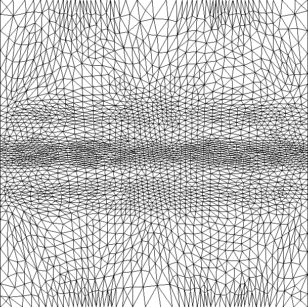
(b) adapted mesh

(c) solution for variable $b$

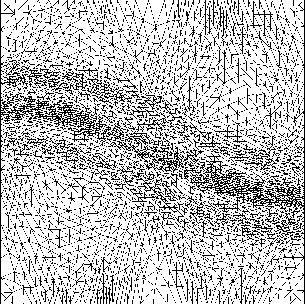
(d) adapted mesh

Figure 2: Exact solution and meshes obtained after 15 iterations for $TOL=0.125$ with $\varepsilon=1$ for constant and variable direction of $b$.

constant direction of $b$ ($\alpha=0$), large anisotropy $\varepsilon=10^{-10}$

In the next test case we consider large anisotropy $\varepsilon=10^{-10}$ and aligned $b$ direction. The simplified error indicator and the full error indicator are no longer equivalent. The results presented in Table 5 display the true error and effectivity indexes obtained by applying those two different algorithms. In this particular case we display results after 30 mesh adaptations. The number is bigger than in previous case in order to allow the algorithm to fully converge and exploit the reduced dimensionality of this particular test. Note that in both cases the true error is comparable and converges with $TOL$. The Zienkiewicz-Zhu effectivity index is close to 1 for both error indicator. The aspect ratio for the smallest $TOL$ studied is over 500. The simplified error indicator seems to perform better : the mesh size for the smallest $TOL$ tested is three times smaller than for the full error indicator. The relative $H^{1}$ error is also slightly smaller for the simplified error indicator. The adapted meshes are presented on Figure 3.

Numerical relative error obtained on the isotropic uniform mesh with $h=0.00625$ (31325 mesh points) give the relative error equal to $0.035$, which is comparable with the results obtained for $TOL=0.0625$. The adapted giving the same numerical precision are 115 (40) times smaller for the simplified (full) error indicator.

(a) solution

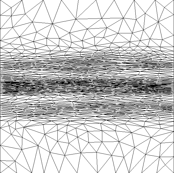
(b) full error indicator

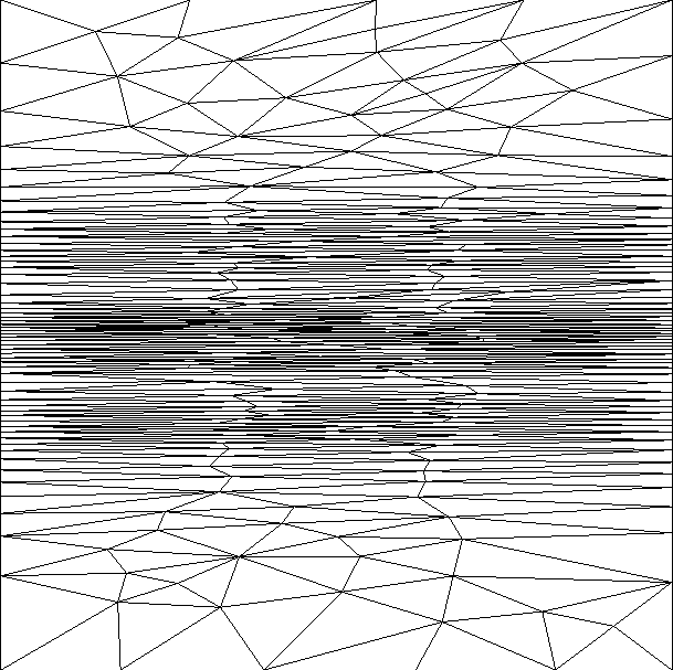
(c) simplified error indicator

Figure 3: Exact solution and meshes obtained after 30 iterations for $TOL=0.125$ with $\varepsilon=10^{-10}$ and constant direction of $b$.

$TOL$	$err$	$NV$	$(\frac{h_{2}}{h_{1}})_{max}$	$(\frac{h_{2}}{h_{1}})_{avg}$	$ei^{ZZ}$	$ei^{A}$
0.25	0.072	272	67	12	1.01	3.20
0.125	0.037	758	86	14	1.01	3.26
0.0625	0.018	2435	91	17	0.99	3.32
0.03125	0.0093	6642	296	23	0.98	3.28

full error indicator

$TOL$	$err$	$NV$	$(\frac{h_{2}}{h_{1}})_{max}$	$(\frac{h_{2}}{h_{1}})_{avg}$	$ei^{ZZ}$	$ei^{SA}$
0.25	0.060	105	130	35	1.01	3.65
0.125	0.031	271	224	48	1.00	3.49
0.0625	0.016	652	501	87	0.98	3.74
0.03125	0.0076	2018	536	106	0.99	4.07

simplified error indicator

Table 5: Relative $H^{1}$ error ($err$), number of nodes ($NV$), maximum aspect ration ($(\frac{h_{2}}{h_{1}})_{max}$), average aspect ration ($(\frac{h_{2}}{h_{1}})_{avg}$) and effectivity indices for mesh iteration $30$ for constant direction of $b$ and $\varepsilon=10^{-10}$

variable direction of $b$ ($\alpha=2$), large anisotropy $\varepsilon=10^{-10}$

In the last studied test case we have applied the mesh adaptation algorithm to the problem with large anisotropy with variable direction. Table 6 shows obtained results of numerical simulations. The simplified error indicator performs more efficiently than the full error indicator. Poor performance of the full error indicator for the smallest tolerance is caused by the perpendicular derivatives of $q^{\varepsilon}_{h}$ which cause the over refinement in the direction perpendicular to the anisotropy direction. The resulting mesh is almost eight times bigger. For smaller values of the tolerance the difference in mesh sizes is much smaller and the meshes constructed for the full error indicator give slightly better precision. In both cases the Z-Z error estimator is close to 1. The adapted meshes are presented on Figure 4.

Numerical relative error obtained on the isotropic uniform mesh with $h=0.00625$ (31325 mesh points) give the relative error equal to $0.038$, which is comparable with the results obtained for $TOL=0.0625$. The adapted giving the same numerical precision are 20 (10) times smaller for the simplified (full) error indicator.

(a) solution

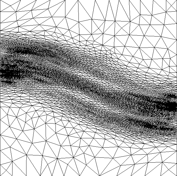
(b) full error indicator

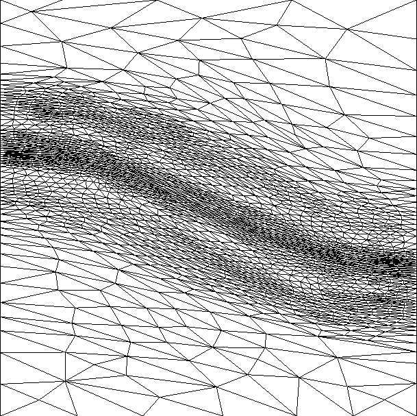
(c) simplified error indicator

Figure 4: Exact solution and meshes obtained after 30 iterations for $TOL=0.125$ with $\varepsilon=10^{-10}$ and variable direction of $b$.

$TOL$	$err$	$NV$	$(\frac{h_{2}}{h_{1}})_{max}$	$(\frac{h_{2}}{h_{1}})_{avg}$	$ei^{ZZ}$	$ei^{A}$
0.5	0.137	183	16	5.4	1.04	3.21
0.25	0.070	587	21	5.8	1.01	3.45
0.125	0.033	3195	54	8.2	0.99	3.83
0.0625	0.015	52658	165	17	0.98	4.88

full error indicator

$TOL$	$err$	$NV$	$(\frac{h_{2}}{h_{1}})_{max}$	$(\frac{h_{2}}{h_{1}})_{avg}$	$ei^{ZZ}$	$ei^{A}$
0.5	0.15	138	27	5.98	1.03	3.18
0.25	0.073	445	25	6.88	1.01	3.34
0.125	0.037	1720	33	7.07	1.00	3.29
0.0625	0.018	6884	43	7.48	0.97	3.36

simplified error indicator

Table 6: Relative $H^{1}$ error ($err$), number of nodes ($NV$), maximum aspect ration ($(\frac{h_{2}}{h_{1}})_{max}$), average aspect ration ($(\frac{h_{2}}{h_{1}})_{avg}$) and effectivity indices for mesh iteration $15$ for variable direction of $b$ and $\varepsilon=10^{-10}$

6 Conclusion

A stabilized Asymptotic Preserving method for strongly anisotropic Laplace equation has been proposed and tested numerically. The error indicators including first order derivatives has been developed for this reformulated problem. Numerical experiments show the performance of the remeshing routine. The resulting meshes are considerably smaller by the factor from 3 to 115 than the isotropic uniform grids giving the same precision. The biggest gain is obtained for strong anisotropy in the constant direction.

References

- [1] J. Adam, J. Boeuf, N. Dubuit, M. Dudeck, L. Garrigues, D. Gresillon, A. Heron, G. Hagelaar, V. Kulaev, N. Lemoine, et al. Physics, simulation and diagnostics of Hall effect thrusters. Plasma Physics and Controlled Fusion, 50:124041, 2008.
- [2] M. Ainsworth and J. T. Oden. A posteriori error estimation in finite element analysis. Comput. Methods Appl. Mech. Engrg., 142(1-2):1–88, 1997.
- [3] M. Ainsworth, J. Z. Zhu, A. W. Craig, and O. C. Zienkiewicz. Analysis of the Zienkiewicz-Zhu a posteriori error estimator in the finite element method. Internat. J. Numer. Methods Engrg., 28(9):2161–2174, 1989.
- [4] S. F. Ashby, W. J. Bosl, R. D. Falgout, S. G. Smith, A. F. Tompson, and T. J. Williams. A Numerical Simulation of Groundwater Flow and Contaminant Transport on the CRAY T3D and C90 Supercomputers. International Journal of High Performance Computing Applications, 13(1):80–93, 1999.
- [5] M. Beer, S. Cowley, and G. Hammett. Field-aligned coordinates for nonlinear simulations of tokamak turbulence. Physics of Plasmas, 2(7):2687, 1995.
- [6] C. Besse, F. Deluzet, C. Negulescu, and C. Yang. Three dimensional simulation of ionsphoric plasma disturbences. in preparation.
- [7] H. Borouchaki and P. Laug. The bl2d mesh generator: Beginner’s guide, user’s and programmer’s manua l. Technical Report RT-0194, Institut National de Recherche en Informatique et Automatique (INRIA), Rocquencourt, 78153 Le Chesnay, France, 1996.
- [8] F. Brezzi and J. Douglas, Jr. Stabilized mixed methods for the Stokes problem. Numer. Math., 53(1-2):225–235, 1988.
- [9] E. Burman and M. Picasso. Anisotropic, adaptive finite elements for the computation of a solutal dendrite. Interfaces Free Bound., 5(2):103–127, 2003.
- [10] P. Degond, F. Deluzet, A. Lozinski, J. Narski, and C. Negulescu. Duality-based asymptotic-preserving method for highly anisotropic diffusion equations. Commun. Math. Sci., 10(1):1–31, 2012.
- [11] P. Degond, F. Deluzet, L. Navoret, A.-B. Sun, and M.-H. Vignal. Asymptotic-preserving particle-in-cell method for the vlasov-poisson system near quasineutrality. J. Comput. Phys., 229(16):5630–5652, 2010.
- [12] P. Degond, F. Deluzet, and C. Negulescu. An asymptotic preserving scheme for strongly anisotropic elliptic problems. Multiscale Model. Simul., 8(2):645–666, 2009/10.
- [13] P. Degond, F. Deluzet, A. Sangam, and M.-H. Vignal. An asymptotic preserving scheme for the Euler equations in a strong magnetic field. J. Comput. Phys., 228(10):3540–3558, 2009.
- [14] P. Degond, A. Lozinski, J. Narski, and C. Negulescu. An asymptotic-preserving method for highly anisotropic elliptic equations based on a micro-macro decomposition. J. Comput. Phys., 231(7):2724–2740, 2012.
- [15] L. Formaggia and S. Perotto. New anisotropic a priori error estimates. Numer. Math., 89(4):641–667, 2001.
- [16] L. Formaggia and S. Perotto. Anisotropic error estimates for elliptic problems. Numer. Math., 94(1):67–92, 2003.
- [17] T. Y. Hou and X.-H. Wu. A multiscale finite element method for elliptic problems in composite materials and porous media. J. Comput. Phys., 134(1):169–189, 1997.
- [18] S. Jin. Efficient asymptotic-preserving (AP) schemes for some multiscale kinetic equations. SIAM J. Sci. Comput., 21(2):441–454, 1999.
- [19] M. Kelley, W. Swartz, and J. Makela. Mid-latitude ionospheric fluctuation spectra due to secondary EŨB instabilities. Journal of Atmospheric and Solar-Terrestrial Physics, 66(17):1559–1565, 2004.
- [20] M. Keskinen, S. Ossakow, and B. Fejer. Three-dimensional nonlinear evolution of equatorial ionospheric spread-F bubbles. Geophys. Res. Lett, 30(16):4–1–4–4, 2003.
- [21] T. Manku and A. Nathan. Electrical properties of silicon under nonuniform stress. Journal of Applied Physics, 74(3):1832–1837, 1993.
- [22] S. Micheletti, S. Perotto, and M. Picasso. Stabilized finite elements on anisotropic meshes: a priori error estimates for the advection-diffusion and the Stokes problems. SIAM J. Numer. Anal., 41(3):1131–1162 (electronic), 2003.
- [23] M. Picasso. An anisotropic error indicator based on Zienkiewicz-Zhu error estimator: application to elliptic and parabolic problems. SIAM J. Sci. Comput., 24(4):1328–1355 (electronic), 2003.
- [24] M. Picasso. Numerical study of the effectivity index for an anisotropic error indicator based on Zienkiewicz-Zhu error estimator. Comm. Numer. Methods Engrg., 19(1):13–23, 2003.
- [25] M. Picasso. Adaptive finite elements with large aspect ratio based on an anisotropic error estimator involving first order derivatives. Comput. Methods Appl. Mech. Engrg., 196(1-3):14–23, 2006.
- [26] R. Rodríguez. Some remarks on Zienkiewicz-Zhu estimator. Numer. Methods Partial Differential Equations, 10(5):625–635, 1994.
- [27] A. M. Tréguier. Modélisation numérique pour l’océanographie physique. Ann. Math. Blaise Pascal, 9(2):345–361, 2002.
- [28] W.-W. Wang and X.-C. Feng. Anisotropic diffusion with nonlinear structure tensor. Multiscale Model. Simul., 7(2):963–977, 2008.
- [29] J. Weickert. Anisotropic diffusion in image processing. European Consortium for Mathematics in Industry. B. G. Teubner, Stuttgart, 1998.
- [30] O. C. Zienkiewicz and J. Z. Zhu. A simple error estimator and adaptive procedure for practical engineering analysis. Internat. J. Numer. Methods Engrg., 24(2):337–357, 1987.
- [31] O. C. Zienkiewicz and J. Z. Zhu. The superconvergent patch recovery and a posteriori error estimates. I. The recovery technique. Internat. J. Numer. Methods Engrg., 33(7):1331–1364, 1992.