$\pi^{+}\pi^{-}$ and $\pi^{0}\pi^{0}$ pair production in photon-photon
and in ultraperipheral ultrarelativistic heavy ion collisions

Abstract

We discuss $\gamma\gamma\to\pi\pi$ reactions, starting from the two-pion threshold up to about $\sqrt{s_{\gamma\gamma}}$ = 6 GeV. Several reaction mechanisms are identified. We include the dipion continuum due to pion exchange (for $\pi^{+}\pi^{-}$) and $\rho^{\pm}$ exchange (for $\pi^{0}\pi^{0}$) as well as the pronounced dipion $\sigma(600)$, $f_{0}(980)$ and $f_{2}(1270)$ s-channel resonances. We discuss also a possible contribution of less pronounced scalar resonances $f_{0}(1500)$ and $f_{0}(1710)$ being glueball candidates, as well as the tensor the resonances $f^{\prime}_{2}(1525)$, $f_{2}(1565)$ and $f_{2}(1950)$. While the contribution of $f^{\prime}_{2}(1525)$ is rather small, the contribution of $f_{2}(1565)$ changes the spectrum around the resonance position. We find that the inclusion of the spin-four $f_{4}(2050)$ resonant state improves the situation at $\sqrt{s_{\gamma\gamma}}\approx$ 2 GeV. We estimate the relevant diphoton partial decay width to be $\Gamma_{f_{4}\to\gamma\gamma}\approx$ 0.7 keV. At higher energies, Brodsky-Lepage and hand-bag mechanisms are included in addition. We nicely describe the world data for $\gamma\gamma\to\pi\pi$ for the first time both for the total cross section and angular distributions for $\gamma\gamma\to\pi^{+}\pi^{-}$ and $\gamma\gamma\to\pi^{0}\pi^{0}$ reactions simultaneously at all experimentally available energies.

The cross section for the production of two-pions in ultraperipheral ultrarelativistic heavy ion collisions is calculated in the impact parameter space Equivalent Photon Approximation (EPA). We obtain the nuclear cross section of 46.7 mb for $\pi^{+}\pi^{-}$ and 8.7 mb for $\pi^{0}\pi^{0}$ at the LHC energy $\sqrt{s_{NN}}=$ 3.5 TeV and minimal cut on pion transverse momentum $p_{t}>$ 0.2 GeV. Differential distributions in impact parameter, dipion invariant mass, single pion and dipion rapidity, pion transverse momentum as well as pion pseudorapidity are shown. The $\gamma\gamma\to\pi^{+}\pi^{-}$ subprocess constitutes a background to the exclusive $AA\to A\rho^{0}(\to\pi^{+}\pi^{-})A$ process, initiated by photon-pomeron or pomeron-photon subprocesses. We find that only a part of the dipion invariant mass spectrum associated with $\gamma\gamma$-collisions can be potentially visible as the cross section for the $AA\to A\rho^{0}A$ reaction is very large.

I Introduction

Ultrarelativistic ultraperipheral production of mesons and elementary particles is a special category of nuclear reactions nucl_reac . The ultrarelativistic ions provide large fluxes of quasi-real photons which can collide leading to different final states. Both total photon-photon cross sections as well as cross section for particular simple final states are interesting. The nuclear cross section is usually calculated in the Equivalent Photon Approximation in momentum space Serbo ; KS_muon , or in impact parameter space BF90 ; KS_muon . In the latter case the flux of photons depends on the transverse distance from the heavy ion trajectory. Impact parameter space is very convenient to exclude cases when both heavy ions collide, i.e., when they do not survive the high-energy collision. In the past we have performed also full momentum space calculation for $\mu^{+}\mu^{-}$ production KS_muon . In the momentum space calculation (EPA or full calculation) the effects of nucleus-nucleus collisions and their associated break-up are neglected. This effect is rather small for light particle production such as $e^{+}e^{-}$ often studied in the literature.

Recently we have studied several processes initiated by the photon-photon collisions such as: $\rho^{0}\rho^{0}$ KS_rho , $\mu^{+}\mu^{-}$ KS_muon , $Q\bar{Q}$ KS_quarks , $D\bar{D}$ LS_DD and for high mass dipions KS_pQCD . We have shown there that the inclusion of realistic charge form factors, being Fourier transforms of realistic charge distributions, is crucial for estimating reliably the nuclear cross sections.

Here, we shall apply the previously used method for the exclusive production of $\pi^{+}\pi^{-}$ and $\pi^{0}\pi^{0}$. The present analysis is an extension of the analysis of high-mass dipion production KS_pQCD where we concentrated exclusively on perturbative QCD effects.

The elementary reactions $\gamma\gamma\to\pi^{0}\pi^{0}$ and $\gamma\gamma\to\pi^{+}\pi^{-}$ are interesting by themselves, since understanding the mechanism of the $\gamma\gamma\to\pi\pi$ reaction at low or intermediate energies ($\sqrt{s_{\gamma\gamma}}<$ 1.5 GeV) is very important for applications of chiral perturbation theory and pion-pion interaction low_energy ; Achasov ; AS2008 ; Ko ; MNW ; Pennington . At higher photon-photon energies the Brodsky-Lepage BL81 ; JA ; SS03 ; QCD_hb ; KS_pQCD and hand-bag HB mechanisms have been discussed in the literature.

In addition, we study the contribution of glueballs or glueball candidates ALEPH_glueball . Only estimates of the total cross section were presented in the literature Machado_glueball recently. In general, it is not possible to observe glueballs, even if the corresponding cross section is sizeable. One should concentrate on a concrete final state. The $\pi\pi$ channels are a good example. Estimation of the background and its interplay with resonant signal should be better understood. Here we show how the glueball candidates can be seen in reality when analyzing e.g. dipion spectra.

In the present paper we construct a hybrid, multi-component model for the $\gamma\gamma\to\pi\pi$ reactions which describes all experimentally available world data. We shall extend the range of the photon-photon energies to the region where the transition from nonperturbative QCD to pQCD may be expected. It is very important to understand the onset of the pQCD effects. For example the hand-bag mechanism HB is usually fitted to experimental data for energies bigger than 2.5 GeV.

The $\gamma\gamma\to\pi\pi$ processes are fairly complicated. Different mechanisms may contribute in general. The present analysis is partially an update of an old analysis in Ref.SS03 . In the present paper we shall try to understand both $\gamma\gamma\to\pi^{+}\pi^{-}$ as well as $\gamma\gamma\to\pi^{0}\pi^{0}$ processes simultaneously, from the kinematical threshold ($W=2m_{\pi}$) up to the maximal experimentally available energy $W_{\gamma\gamma}\approx$ 6 GeV. We will include both soft and hard continuum processes as well as s-channel resonances. Here we shall include many more resonances compared to Ref.SS03 . In addition, we shall try to describe the new very precise data of the Belle Collaboration Belle_Uehara09 , including the angular distributions of pions.

Our paper concentrates on realistic predictions of the cross sections for dipion production in ultraperipheral ultrarelativistic heavy ion collisions. We shall present first realistic predictions for $PbPb\to Pb(\pi\pi)Pb$ reaction at the LHC. Both total cross sections and differential distributions will be shown and discussed for the first time in the literature. The photon-photon induced dipion production in nuclear collision, interesting by itself, constitutes a background to another type of nucleus-nucleus reactions induced by photon-pomeron (pomeron-photon) exchanges leading to a coherent production of $\rho^{0}$ meson Grube_STAR ; BKN2002 ; FSZ2002 and its radial excitations. The interplay of the both processes was not discussed so far in the literature.

II Modelling $\gamma\gamma\to\pi\pi$ reactions

II.1 The $\gamma\gamma\to\pi^{+}\pi^{-}$ continuum

The Born amplitude for the $\gamma\gamma\to\pi^{+}\pi^{-}$ process is shown in Fig.1.

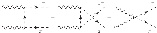
Figure 1: The Born term matrix elements for non resonant pion pair production.

The helicity dependent amplitude for point-like pions is a sum of the three terms (see e.g. Brodsky1971 ):
contact amplitude:

$$\mathcal{M}_{\lambda_{1}\lambda_{2}}^{\pi,c}\left(q_{1},q_{2},p_{\pi^{+}},p_{\pi^{-}}\right)=e^{2}\sum 2g^{\mu\nu}\varepsilon_{\mu}(\lambda_{1})\varepsilon_{\nu}(\lambda_{2})\;,$$ (1)

t-channel pion-exchange amplitude:

$$\mathcal{M}_{\lambda_{1}\lambda_{2}}^{\pi,t}\left(q_{1},q_{2},p_{\pi^{+}},p_{\pi^{-}}\right)=e^{2}\sum\left(2p_{\pi^{-}}^{\mu}-q_{1}^{\mu}\right)\varepsilon_{\mu}(q_{1},\lambda_{1})\left(2p_{\pi^{+}}^{\nu}-q_{2}^{\nu}\right)\varepsilon_{\nu}(q_{2},\lambda_{2})\frac{1}{t-m_{\pi}^{2}}\;$$ (2)

and u-channel pion-exchange amplitude:

$$\mathcal{M}_{\lambda_{1}\lambda_{2}}^{\pi,u}\left(q_{1},q_{2},p_{\pi^{+}},p_{\pi^{-}}\right)=e^{2}\sum\left(2p_{\pi^{+}}^{\mu}-q_{1}^{\mu}\right)\varepsilon_{\mu}(q_{1},\lambda_{1})\left(2p_{\pi^{-}}^{\nu}-q_{2}^{\nu}\right)\varepsilon_{\nu}(q_{2},\lambda_{2})\frac{1}{u-m_{\pi}^{2}}\;.$$ (3)

The full pion-exchange amplitude is a sum of contact + t + u amplitudes

$$\mathcal{M}_{\lambda_{1}\lambda_{2}}^{\pi}=\mathcal{M}_{\lambda_{1}\lambda_{2}}^{\pi,c}+\mathcal{M}_{\lambda_{1}\lambda_{2}}^{\pi,t}+\mathcal{M}_{\lambda_{1}\lambda_{2}}^{\pi,u}\;.$$ (4)

Such an amplitude can be formally written as:

$$\mathcal{M}_{\lambda_{1}\lambda_{2}}^{\pi}=\varepsilon_{\mu}(q_{1},\lambda_{1})\varepsilon_{\nu}(q_{2},\lambda_{2})\mathcal{M}^{\mu\nu}\;.$$ (5)

It is straightforward to show that

$$q_{1\mu}\mathcal{M}^{\pi,\mu\nu}=0,$$

$$q_{2\mu}\mathcal{M}^{\pi,\mu\nu}=0\;,$$ (6)

which is consistent with gauge invariance. The QED Born amplitude for the $\gamma\gamma\to\pi^{+}\pi^{-}$ reaction with point-like particles has been known for a long time. An interesting problem is to construct the QED amplitude for real, finite-size, pions. We use an idea proposed by Poppe Poppe , and correct the QED amplitude by an overall $t$ and $u$ dependent form factor:

$$\mathcal{M}_{\lambda_{1},\lambda_{2}}^{\pi}\left(t,u,s\right)=\Omega\left(t,u,s\right)\mathcal{M}_{\lambda_{1},\lambda_{2}}^{\pi,QED}\left(t,u,s\right)\;.$$ (7)

It is natural that finite size corrections damp the QED amplitude for both $t$ and $u$ large. At sufficiently high energies the following simplification fulfils this requirement:

$$\Omega\left(t,u,s\right)=\frac{F^{2}\left(t\right)+F^{2}\left(u\right)}{1+F^{2}\left(-s\right)}\;.$$ (8)

In practice one can take $F(x)=\exp(\frac{B_{\gamma\pi}}{4}x)$; $B_{\gamma\pi}=$ (4-6) GeV^-2. $F(x)$ denotes the standard vertex function which provides the convenient normalization $F\left(0\right)$ = 1 and additionally $F\left(t\right)\to$ 0 when $t\to-\infty$. In the limit of large $s$:

$$\Omega\left(t,u,s\right) \stackrel{{\scriptstyle t\to 0}}{{\longrightarrow}} F^{2}\left(t\right)\;,$$

$$\Omega\left(t,u,s\right) \stackrel{{\scriptstyle u\to 0}}{{\longrightarrow}} F^{2}\left(u\right)\;.$$ (9)

This $s$ limit generates standard vertex form factors and additionally at $z\equiv\cos\theta\approx 0$:

$$\frac{d\sigma^{\pi}}{dz}\left(z=0,s\right)\propto F^{4}\left(\frac{-s}{2}\right)\;.$$ (10)

II.2 $s$-channel $\gamma\gamma\to$ resonances

In Fig.2 we show a list of several possible dipion resonances that could, in principle, contribute to the $\gamma\gamma\to\pi\pi$ processes.

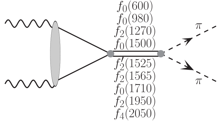
Figure 2: $\gamma\gamma\to\mbox{resonances}\to\pi^{+/0}\pi^{-/0}$.

Table 1: Parameters of resonances used in our calculations.

Resonance	$m_{R}$ (MeV)	$\Gamma_{R}$ (MeV)	$\Gamma_{\pi\pi}$ (MeV)	$\Gamma_{\gamma\gamma}$ (keV)	$\frac{\Gamma_{\gamma\gamma}\Gamma_{\pi\pi}}{\Gamma_{R}}$ (keV)
$f_{0}(600)$ PDG	600	400	400	0.5
$f_{0}(980)$ PDG	980	50	51.3 Belle_Mori	0.29
$f_{2}(1270)$ PDG	1 275	185	156.9	3.035
$f_{0}(1500)$ PDG	1 505	109	38	-	0.033 Belle_Uehara08
$f^{\prime}_{2}(1525)$ PDG	1 525	73	0.6	0.081
$f_{2}(1565)$ Schegelsky	1 570	160	25	0.7
$f_{0}(1710)$ PDG	1 720	135	-	-	0.82
$f_{2}(1950)$ PDG	1 944	472	-	-	1.62
$f_{4}(2050)$ PDG	2 018	237	40.3	0.7

In Table 1 we have collected these resonances with parameters known from Particle Data Group book PDG . In the present analysis we shall take into account the following scalar: $\sigma(600)$, $f_{0}(980)$, $f_{0}(1500)$, $f_{0}(1710)$, tensor: $f_{2}(1270)$, $f^{\prime}_{2}(1525)$, $f_{2}(1565)$, $f_{2}(1950)$ as well as spin-4: $f_{4}(2050)$ resonances. While the $\pi\pi$ decay widths are usually well known, the $\gamma\gamma$ decay widths are known only for some of them. Therefore, studying the $\gamma\gamma\to\pi\pi$ data may help in extracting the latter quantities. Below we shall present both, theoretical estimates of some of them, as well as a fit to experimental total cross sections and angular distributions.

In most cases, PDG gives values of the resonance parameters: $m_{R}$, $\Gamma_{R}$, $\Gamma_{\pi\pi}$ and $\Gamma_{\gamma\gamma}$. We use somewhat smaller values of decay widths for $f_{0}(600)$ resonance than given in the PDG book. In the PDG book PDG a broad range of parameters is given: $\Gamma_{R}$=(600-1000) MeV, $\Gamma_{\gamma\gamma}$ =(1.2-10) keV. In our case we find: $\Gamma_{R}$=400 MeV, $\Gamma_{\gamma\gamma}$ =0.5 keV as the best fit parameters. In addition, we assume that Br($f_{0}(600)\to\pi\pi$)=100%. For $f_{0}(1500)$ PDG gives $\frac{\Gamma_{\gamma\gamma}\Gamma_{\pi\pi}}{\Gamma_{R}}$=0.033 keV which was obtained by the Belle Collaboration which includes in addition in their fit the $f_{0}(1370)$ resonance Belle_Uehara08 . Using this value, we obtain: $\Gamma_{\gamma\gamma}$=0.1 keV. For $f_{4}(2050)$ the situation is even more complicated. Different values of the ratio (see last column in Table 1) has been given in the literature: Belle_Uehara09 : $\frac{\Gamma_{\gamma\gamma}\Gamma_{\pi\pi}}{\Gamma_{R}}$=0.0231 keV, Oest : $\frac{\Gamma_{\gamma\gamma}\Gamma_{\pi\pi}}{\Gamma_{R}}<$ 1.1 keV. In our fit to the Belle experimental data (to be shown in the Result section) we find: $\frac{\Gamma_{\gamma\gamma}\Gamma_{\pi\pi}}{\Gamma_{R}}$ = 0.12 keV.

The angular distribution for the s-channel resonances can be written in the standard (typical for Feynman-diagrams) form:

$$\frac{d\sigma\left(\gamma\gamma\to\pi\pi\right)}{dz}=\sum_{\lambda_{1},\lambda_{2}}\frac{\sqrt{\frac{W^{2}}{4}-m_{\pi}^{2}}}{\frac{W}{2}}\left|\mathcal{M}\left(\lambda_{1},\lambda_{2}\right)\right|^{2}\frac{4\pi}{4\times 64\pi^{2}W^{2}}\;,$$ (11)

where the helicity-dependent resonant amplitudes must be modelled, as we do not have a priori microscopic models of the coupling of two photons to high-spin resonances. Our parameterizations for the $f_{0}$, $f_{2}$ and $f_{4}$ resonances are:

$$\mathcal{M}\left(\lambda_{1},\lambda_{2}\right) = \frac{\sqrt{64\pi^{2}W^{2}\times 8\pi\left(2J+1\right)\left(\frac{m_{R}}{W}\right)^{2}\Gamma_{R}\Gamma_{R}\left(W\right)Br\left(R\to\gamma\gamma\right)Br\left(R\to\pi^{+/0}\pi^{-/0}\right)}}{W^{2}-m_{R}^{2}+im_{R}\Gamma_{R}\left(W\right)}e^{i\varphi_{R}}$$ (16)

$$\times \sqrt{2}\delta_{\lambda_{1},\lambda_{2}}\left\{\begin{array}[]{l}Y^{0}_{0};\mbox{for }f_{0}\\ Y^{2}_{2};\mbox{for }f_{2}(1270),f^{\prime}_{2}(1525),f_{2}(1950)\\ Y^{0}_{2};\mbox{for }f_{2}(1565)\\ Y^{0}_{4};\mbox{for }f_{4}(2050)\end{array}\right\}\times\exp\left(\frac{-\left(W-m_{R}\right)^{2}}{\Lambda_{R}^{2}}\right)\;.$$

The last (form)factor was introduced to correct the resonance form far from the actual resonance position where the simple resonance form is incorrect. We expect $\Lambda_{R}$ to be much larger than the resonance width $\Gamma_{R}$. In practice we will treat it as an extra free parameter to be adjusted to experimental data. This has importance only for broad resonances with $\Gamma>$ 0.1 GeV.

The energy-dependent resonance widths are parametrized as:

$$\Gamma_{R}(W)=\Gamma_{R}\frac{\sqrt{\frac{W^{2}}{4}-m_{\pi}^{2}}}{\sqrt{\frac{m_{R}^{2}}{4}-m_{\pi}^{2}}}F^{J}\left(W,R\right)\;,$$ (17)

where the function $F^{J}\left(W,R\right)$ is the spin dependent Blatt-Weisskopf form factor BW1952 :

$$F^{J=0}\left(W,R\right) = 1,$$

$$F^{J=2}\left(W,R\right) = \frac{\left(Rp_{R}\right)^{4}+3\left(Rp_{R}\right)^{2}+9}{\left(Rp\right)^{4}+3\left(Rp\right)^{2}+9},$$

$$F^{J=4}\left(W,R\right) = \frac{\left(Rp_{R}\right)^{8}+10\left(Rp_{R}\right)^{6}+135\left(Rp_{R}\right)^{4}+1575\left(Rp_{R}\right)^{2}+11025}{\left(Rp\right)^{8}+10\left(Rp\right)^{6}+135\left(Rp\right)^{4}+1575\left(Rp\right)^{2}+11025}\;.$$ (18)

Above $p_{R}=\sqrt{\frac{m_{R}^{2}}{4}-m_{\pi}^{2}}$, $p=\sqrt{\frac{W^{2}}{4}-m_{\pi}^{2}}$ and R = 1 fm.

The decay of $f_{2}(1565)$ into dipions was studied first in Ref.Crystal_Barrel by the Crystal Barrel Collaboration, while its decay into two photons was studied in Ref.Schegelsky . The $f_{4}(2050)$ resonance was not studied so far in $\gamma\gamma\to\pi\pi$ reactions.

We consider two simple models of the amplitude for the tensor meson production:

$${\cal M}_{\lambda_{1}\lambda_{2}}^{J=2} \propto Y_{2,\lambda_{1}-\lambda_{2}}(\theta,\phi)\cdot\left(\delta_{\lambda_{1}-\lambda_{2},-2}+\delta_{\lambda_{1}-\lambda_{2},2}\right)\;{\mbox{(type A)}},$$

$${\cal M}_{\lambda_{1}\lambda_{2}}^{J=2} \propto Y_{2,\lambda_{1}-\lambda_{2}}(\theta,\phi)\cdot\delta_{\lambda_{1}-\lambda_{2},0}\;{\mbox{(type B)}}.$$ (19)

We shall call them model A and B, respectively.

For $f_{2}(1270)$ production the amplitude is dominantly of the type A Poppe . We assume the same for the $f^{\prime}_{2}(1525)$ and $f_{2}(1950)$ resonances since they are the same nonet partners of $f_{2}(1270)$.

The $f_{2}(1565)$ resonance is not well understood so far. The Belle Collaboration finds in this region both components (A, B) in the partial wave analysis Belle_Uehara09 ; Belle_Uehara08 ; Belle_Mori . We shall try both models in order to describe the experimental data, taking the $\Gamma_{\pi\pi}$ decay width from Schegelsky and fitting $\Gamma_{\gamma\gamma}$.

For the spin-4 resonance again two simple possibilities come into the game:

$${\cal M}_{\lambda_{1}\lambda_{2}}^{J=4} \propto Y_{4,\lambda_{1}-\lambda_{2}}(\theta,\phi)\cdot\left(\delta_{\lambda_{1}-\lambda_{2},-2}+\delta_{\lambda_{1}-\lambda_{2},2}\right)\;{\mbox{(type A)}},$$

$${\cal M}_{\lambda_{1}\lambda_{2}}^{J=4} \propto Y_{4,\lambda_{1}-\lambda_{2}}(\theta,\phi)\cdot\delta_{\lambda_{1}-\lambda_{2},0}\;{\mbox{(type B)}}.$$ (20)

While the Belle partial wave analysis Belle_Uehara09 ; Belle_Uehara08 ; Belle_Mori suggests the dominance of the type A form, in our analysis we find that type B fits better to experimental data.

II.3 $\gamma\gamma\to\pi^{0}\pi^{0}$ in a simple coupled channel model with $\rho^{\pm}$ exchange

Since the cross section for the $\gamma\gamma\to\pi^{+}\pi^{-}$ reaction is much bigger than that for the $\gamma\gamma\to\pi^{0}\pi^{0}$ reaction, even a small coupling between these channels may modify the cross section for the $\gamma\gamma\to\pi^{0}\pi^{0}$ reaction. An example of a process which leads to channel coupling is shown in Fig.3.

Figure 3: $\gamma\gamma\to\pi^{+}\pi^{-}\to\rho\to\pi^{0}\pi^{0}$.

The contact amplitude (see diagram (a) in Fig.3) can be written as:

$$\mathcal{M}^{c}(\lambda_{1},\lambda_{2}) = \int 2e^{2}g^{\mu\nu}\epsilon_{\mu}(\lambda_{1})\epsilon_{\nu}(\lambda_{2})\frac{1}{k_{1}^{2}-m_{\pi}^{2}+i\epsilon}g_{\pi\pi\to\rho}\left(k_{1}^{\alpha}+p_{1}^{\alpha}\right)$$ (21)

$$\times \frac{\left(-g_{\alpha\beta}+\frac{{q}_{\alpha}q_{\beta}}{m_{\rho}^{2}}\right)}{\kappa^{2}-m_{\rho}^{2}+i\Gamma_{\rho}m_{\rho}}g_{\pi\pi\to\rho}\left(k_{2}^{\beta}+p_{2}^{\beta}\right)\frac{1}{k_{2}^{2}-m_{\pi}^{2}+i\epsilon}$$

$$\times F(\hat{s},\hat{t},\hat{u})F^{2}(\kappa)F^{2}(k_{1})F^{2}(k_{2})\frac{d^{4}\kappa}{\left(2\pi\right)^{4}}\;$$

and the corresponding t-channel amplitude (see diagram (b) in Fig.3) as:

$$\mathcal{M}^{t}(\lambda_{1},\lambda_{2}) = \int\frac{e^{2}}{\kappa_{2}^{2}-m_{\pi}^{2}+i\epsilon}\frac{1}{k_{1}^{2}-m_{\pi}^{2}+i\epsilon}g_{\pi\pi\to\rho}\left(k_{1}^{\alpha}+p_{1}^{\alpha}\right)$$ (22)

$$\times \frac{\left(-g_{\alpha\beta}+\frac{{q}_{\alpha}q_{\beta}}{m_{\rho}^{2}}\right)}{\kappa^{2}-m_{\rho}^{2}+i\Gamma_{\rho}m_{\rho}}g_{\pi\pi\to\rho}\left(k_{2}^{\beta}+p_{2}^{\beta}\right)\frac{1}{k_{2}^{2}-m_{\pi}^{2}+i\epsilon}$$

$$\times \epsilon_{\mu}\left(\lambda_{1}\right)\left(\kappa_{2}^{\mu}+k_{1}^{\mu}\right)\epsilon_{\nu}\left(\lambda_{2}\right)\left(\kappa_{2}^{\nu}-k_{2}^{\nu}\right)$$

$$\times F(\hat{s},\hat{t},\hat{u})F^{2}(\kappa)F^{2}(k_{1})F^{2}(k_{2})\frac{d^{4}\kappa}{\left(2\pi\right)^{4}}\;.$$

The form factors that appear in the above formulas are parametrized as:

• $F(\hat{s},\hat{t},\hat{u})=\frac{F^{2}(\hat{t})+F^{2}(\hat{u})}{1+F^{2}(\hat{s})}$,

• $F(x=\hat{s})=\exp\left(\frac{-\left(x-4m_{\pi}^{2}\right)^{2}}{\Lambda^{4}}\right)$,

• $F(x=\hat{t},\hat{u},k_{1},k_{2})=\exp\left(\frac{-\left(x^{2}-m_{\pi}^{2}\right)^{2}}{\Lambda^{4}}\right)$,

• $F(x=\kappa)=\exp\left(\frac{-\left(x^{2}-m_{\rho}^{2}\right)^{2}}{\Lambda^{4}}\right)$,

where $\Lambda$ is, in principle, a free parameter. The resulting amplitude strongly depends on the value of the parameter.

The u-channel amplitude can be obtained from the t-channel amplitude by interchanging $\pi^{+}$ and $\pi^{-}$ ($\mathcal{M}^{u}\left(\lambda_{1},\lambda_{2}\right)=\mathcal{M}^{t}\left(\lambda_{1},\lambda_{2}\right)$).
The corresponding distribution in $z=\cos\theta$, when artificially separating the process, can be obtained from the amplitudes as usually:

$$\frac{d\sigma}{dz}=\sum_{\lambda_{1},\lambda_{2}}\frac{\sqrt{\frac{W^{2}}{4}-m_{\pi}^{2}}}{\frac{W}{2}}\left|\mathcal{M}^{t}(\lambda_{1},\lambda_{2})+\mathcal{M}^{u}(\lambda_{1},\lambda_{2})+\mathcal{M}^{c}(\lambda_{1},\lambda_{2})\right|^{2}\frac{4\pi}{4\times 64\pi^{2}W^{2}}\;.$$ (23)

II.4 pQCD mechanisms

In Ref.KS_pQCD we have concentrated on perturbative mechanisms. In the present paper we shall only summarize the main formulae. Again, as shown in Fig.4, we shall consider simultaneously the $\pi^{+}\pi^{-}$ and $\pi^{0}\pi^{0}$ channels.

Figure 4: The Brodsky-Lepage or hand-bag perturbative mechanisms for large-angle $\gamma\gamma\to\pi\pi$ scattering.

II.4.1 Brodsky-Lepage mechanism

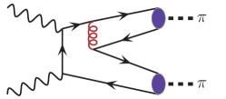
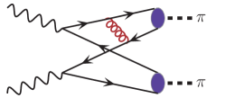
Figure 5: Feynman diagrams describing the $\gamma\gamma\to\pi\pi$ amplitude in LO pQCD.

The basic diagrams of the Brodsky and Lepage formalism are shown in Fig.5. The invariant amplitude for the initial helicities of two photons can be written as:

$$\mathcal{M}\left(\lambda_{1},\lambda_{2}\right)=\int_{0}^{1}dx\int_{0}^{1}dy\,\phi_{\pi}\left(x,\mu^{2}_{x}\right)T^{\lambda_{1}\lambda_{2}}_{H}\left(x,y,\mu^{2}\right)\phi_{\pi}\left(y,\mu^{2}_{y}\right)\times F^{pQCD}_{reg}\left(t,u\right),$$ (24)

where for $\mu_{x}$ or $\mu_{y}$: $\mu_{x_{/y}}=min\left(x_{/y},1-x_{/y}\right)\sqrt{s(1-z^{2})}$; $z=\cos\theta$ BL81 . We take the helicity dependent hard scattering amplitudes from Ref.JA . These scattering amplitudes are different for $\pi^{+}\pi^{-}$ and $\pi^{0}\pi^{0}$. The extra form factor in Eq.24 was proposed in Ref.SS03 :

$$F^{pQCD}_{reg}\left(t,u\right)=\left[1-\exp\left(\frac{t-t_{m}}{\Lambda_{reg}^{2}}\right)\right]\left[1-\exp\left(\frac{u-u_{m}}{\Lambda_{reg}^{2}}\right)\right],$$ (25)

where $t_{m}=u_{m}$ are the maximal kinematically allowed values of $t$ and $u$. This form factor excludes the region of small Mandelstam $t$ and $u$ variables which is clearly of nonperturbative nature. In the present analysis we are even more conservative and try to separate the phase space into low and high energies and postulate that the pQCD effects show up only above a certain energy. In practice we use the following function which smoothly switches off the pQCD contribution at low energies:

$$F^{pQCD}(s)=1-\exp\left(\frac{-\left(s-4m_{\pi}^{2}\right)^{4}}{\Lambda^{8}_{pQCD}}\right)\;.$$ (26)

Figure 6: Comparison of different forms of the extra form factor. We show results for a new separation of low and high energy processes given by Eq.(26) and represented by the red solid line ($\Lambda_{pQCD}=$ 2.5 GeV). In Ref.KS_pQCD we used the form given by Eq.(25) represented in the figure by the green dashed line ($\Lambda_{reg}=$ 1 GeV). The dotted line shows the BL pQCD cross section without any extra form factor.

Fig.6 illustrates the role of the extra form factors discussed above.

The distribution amplitudes are subjected to the ERBL pQCD evolution ER ; BL79 . The scale dependent quark distribution amplitude of the pion Muller ; AB can be expanded in terms of Gegenbauer polynomials:

$$\phi_{\pi}\left(x,\mu^{2}\right)=\frac{f_{\pi}}{2\sqrt{3}}6x\left(1-x\right)\sum_{n=0}^{\infty^{\prime}}C_{n}^{3/2}\left(2x-1\right)a_{n}\left(\mu^{2}\right),$$ (27)

where the expansion coefficients $a_{n}\left(\mu^{2}\right)$ depend on the form of the distribution amplitude $\phi_{\pi}\left(x,\mu_{0}^{2}\right)$. Wu and Huang WH proposed recently a new form of the distribution amplitude:

$$\phi_{\pi}\left(x,\mu_{0}^{2}\right) = \frac{\sqrt{3}A\,m_{q}\beta}{2\sqrt{2}\pi^{3/2}f_{\pi}}\sqrt{x\left(1-x\right)}\left(1+B\times C_{2}^{3/2}\left(2x-1\right)\right)$$ (28)

$$\times \left(\mbox{Erf}\left[\sqrt{\frac{m_{q}^{2}+\mu_{0}^{2}}{8\beta^{2}x\left(1-x\right)}}\right]-\mbox{Erf}\left[\sqrt{\frac{m_{q}^{2}}{8\beta^{2}x\left(1-x\right)}}\right]\right).$$

This pion distribution amplitude at the initial scale ($\mu_{0}^{2}=$ 1 GeV²) is controlled by the parameter B. This simple model better describes recent BABAR data BABAR .

In Fig.7 we compare the results of the Brodsky-Lepage (BL) approach and experimental data for different energies. As can be seen from the figures the BL pQCD approach is not enough to describe the ”high energy” data, especially for the $\gamma\gamma\to\pi^{0}\pi^{0}$ reaction.

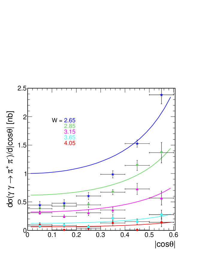
Figure 7: Comparison of BL pQCD angular distributions with Belle data Belle_Nakazawa ; Belle_Uehara09 .

II.4.2 Hand-bag mechanism

The hand-bag approach was proposed in Ref.HB . In this approach the only nonzero helicity-dependent amplitudes read

$$\mathcal{A}_{+-}=\mathcal{A}_{-+}=-4\pi\alpha_{em}\frac{s^{2}}{tu}R_{2\pi}\left(s\right)\;.$$ (29)

The form factors $R_{2\pi}(s)$ are of nonperturbative nature and are in principle unknown. In practice they were fitted to the experimental total (integrated over experimentally measured region) cross section for $\gamma\gamma\to\pi^{+}\pi^{-}$ HB , assuming that the mechanism exhausts the measured cross section at high energy. This is not a necessary condition. In our analysis we shall relax this rather restrictive assumption. In the present paper we discuss also respective angular distributions. We shall use the parametrization proposed in Ref.HB :

$$R_{2\pi}\left(s\right)=\frac{5}{9s}a_{u}\left(\frac{s_{0}}{s}\right)^{n_{u}}+\frac{5}{9s}a_{s}\left(\frac{s_{0}}{s}\right)^{n_{s}}\;.$$ (30)

The values of $a_{u}$, $n_{u}$, $a_{s}$ and $n_{s}$ are taken from Ref.HB . We have averaged the values for different energies: $a_{u}=$ 1.375 GeV², $n_{u}=0.4175$, $a_{s}=$ 0.5025 GeV² and $n_{s}=1.195$.

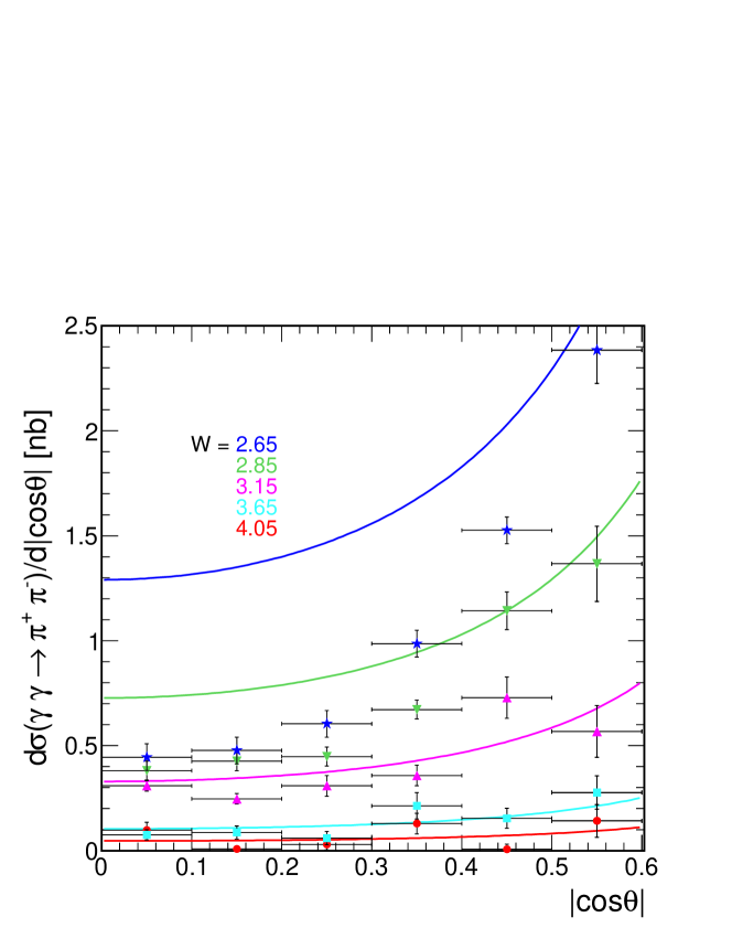
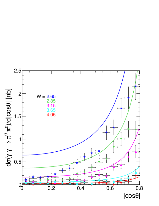
Figure 8: Comparison of hand-bag angular distributions with Belle data Belle_Nakazawa ; Belle_Uehara09 .

In Fig.8 we show angular distributions calculated in the hand-bag approach together with the Belle experimental data Belle_Nakazawa ; Belle_Uehara09 . Only at the highest energies the hand-bag parametrization looks reasonable, however, does not describe properly the ratio of the $\gamma\gamma\to\pi^{0}\pi^{0}$ and $\gamma\gamma\to\pi^{+}\pi^{-}$ cross section (see Fig.14). At somewhat lower energies the hand-bag and experimental distributions differ significantly. The onset of the hand-bag mechanism was not discussed so far in the literature. We shall return to the problem in the Result section where other mechanisms will be discussed too.

II.5 Equivalent photon approximation for $AA\to AA\pi\pi$

How to calculate the production of pairs of particles in nucleus-nucleus collisions was explained in detail in Ref.KS_muon . Here we only sketch the formalism. The total nuclear cross section can be expressed by folding the $\gamma\gamma\to\pi\pi$ subprocess cross section with equivalent photon fluxes as:

$$\sigma(AA\to AA\pi\pi;s_{AA}) = \int\hat{\sigma}(\gamma\gamma\to\pi\pi;W_{\gamma\gamma})S^{2}_{abs}({\bf b})$$ (31)

$$\times N(\omega_{1},{\bf b}_{1})N(\omega_{2},{\bf b}_{2})d^{2}{\bf b}_{1}d^{2}{\bf b}_{2}d\omega_{1}d\omega_{2}\;.$$

In principle, the absorption factor $S_{abs}({\bf b})$ can be calculated in different models. At not too high energies the Glauber approach is a reasonable approach. Here we take a somewhat simpler approach and approximate the absorption factor as:

$$S^{2}_{abs}({\bf b})=\theta({\bf b}-2R_{A})=\theta(|{\bf b}_{1}-{\bf b}_{2}|-2R_{A})\;.$$ (32)

This form excludes the situation at high energies when the colliding nuclei overlap which at high energies unavoidably leads to their breakup.

In order to simplify our calculation we shall use the following transformations:

$$\omega_{1/2}=\frac{W_{\gamma\gamma}}{2}e^{\pm Y_{\pi\pi}}\mbox{, }d\omega_{1}d\omega_{2}=\frac{W_{\gamma\gamma}}{2}dW_{\gamma\gamma}dY_{\pi\pi}\;.$$ (33)

Then formula (31) can be rewritten as:

$$\sigma(AA\to AA\pi\pi;s_{AA}) = \int\hat{\sigma}(\gamma\gamma\to\pi\pi;W_{\gamma\gamma})S^{2}_{abs}({\bf b})$$ (34)

$$\times N(\omega_{1},{\bf b}_{1})N(\omega_{2},{\bf b}_{2})\frac{W_{\gamma\gamma}}{2}d^{2}{\bf b}_{1}d^{2}{\bf b}_{2}dW_{\gamma\gamma}dY_{\pi\pi}\;.$$

While in the above approach one can easily calculate only the total nuclear cross section, distributions in rapidity of the pair of pions, and the invariant mass of the dipions (see e.g. KS_rho ; KS_muon ), experimental constraints can not be easily imposed.

If one wants to calculate in addition kinematical distributions of each of the individual particles (transverse momentum, rapidity, pseudorapidity), or impose corresponding experimental cuts on kinematical quantity of each of dipions, a more complicated calculation is required. Then instead of the one-dimensional array $\sigma(\gamma\gamma\to\pi\pi;W_{i})$, a two-dimensional array $\frac{d\sigma(\gamma\gamma\to\pi\pi)}{dz}\left(W_{i},z_{j}\right)$ has to be calculated, stored and passed to the code calculating cross sections for nuclear collisions. Then an extra integration in $z=\cos\theta$ is required in Eqs. (31) or (34), which makes the calculation much more time-consuming.

Next four-momenta of pions in the $\pi\pi$ center of mass frame are calculated:

$$E_{\pi}=\sqrt{\hat{s}}/2.\;,$$

$$p_{\pi}=\sqrt{\frac{\hat{s}}{4}-m_{\pi}^{2}}\;,$$

$$p_{t,\pi}=\sqrt{1-z^{2}}p_{\pi}\;,$$

$$p_{l}=zp_{\pi}\;.$$ (35)

The rapidity of each of the pions can be calculated easily as:

$$y_{i}=Y_{\pi\pi}+y_{i/\pi\pi}\;,$$ (36)

where $y_{i/\pi\pi}=y_{i/\pi\pi}(W,z)$ is the rapidity of one of the pions in the recoil $\pi\pi$ system of reference. The transverse momenta of pions in both frames of reference, as Lorentz invariants, are the same. Other kinematical variables are calculated by adding relativistically velocities Hagedorn_book

$$\vec{v}_{i}=\vec{V}_{\pi\pi}\oplus\vec{v}_{i/\pi\pi}\;,$$ (37)

where

$$\overrightarrow{V_{\pi\pi}}=\frac{\overrightarrow{P_{\pi\pi}}}{E_{\pi\pi}}$$ (38)

and from the energy-momentum conservation:

$$E_{\pi\pi} = \omega_{1}+\omega_{2}\;,$$

$$P_{\pi\pi}^{z} = \omega_{1}-\omega_{2}\;,$$ (39)

the energies of photons can be expressed in terms of our integration variables as:

$$\omega_{1} = \frac{W_{\gamma\gamma}}{2}\exp(Y)\;,$$

$$\omega_{2} = \frac{W_{\gamma\gamma}}{2}\exp(-Y)\;.$$ (40)

Now the pion velocities can be converted to four-momenta of pions in the overall nucleus-nucleus center of mass frame. Then angles or pseudorapidities of pions can be easily calculated and experimental cuts can be imposed in addition.

Distributions in kinematical variables are obtained by corresponding binning into histograms. A smooth distributions in transverse momenta or pseudorapidities require many points in $W$ and $z$. If only experimental cuts are imposed the number of points can be smaller. In the present approach we are interested first of all in two-pion invariant mass distribution but including cuts of real experiments.

II.6 $AA\to AA\rho$

In nucleus-nucleus collisions another mechanism exists which contributes to the $\pi^{+}\pi^{-}$ channel – coherent production of $\rho^{0}$ mesons and its subsequent decay into the $\pi^{+}\pi^{-}$ channel ($\rho^{0}\to\pi^{+}\pi^{-}$). This mechanism was studied theoretically in the classical Glauber KN99 , quantum Glauber FSZ , Glauber-Gribov FSZ02 ; RSZ2011 and Color Glass Condensate GM11 approaches. The rapidity distribution of $\rho^{0}$ can be written in an almost model-independent way as:

$$\frac{d\sigma}{dy}=\omega_{1}\frac{dN_{\gamma}(\omega_{1})}{d\omega_{1}}\sigma_{\gamma A\to VA}+\omega_{2}\frac{dN_{\gamma}(\omega_{2})}{d\omega_{2}}\sigma_{A\gamma\to AV}\;.$$ (41)

Essentially the models enter in calculating the cross section for $\gamma A\to VA$ processes. While for heavy quarkonium production the situation is more transparent CSS12 , for light meson production the situation is somewhat less certain. We shall not discuss the issue here, we rather refer the reader to the existing literature (see e.g. ultraperiheral ). In the most rudimentary approach:

$$\sigma_{\gamma A\to\rho^{0}A}=\frac{\alpha_{em}}{4f_{\rho}^{2}}\left(\sigma_{\rho A}^{tot}\right)^{2}\int_{t_{min}}^{\infty}dtF_{A}^{2}(t)\;,$$ (42)

where $\sigma_{\rho A}^{tot}\approx\pi R_{A}^{2}$ and $t_{min}=\frac{m_{\rho}^{4}}{4q_{0}^{2}}$ FSZ .

III Results

Before we go to the nuclear processes we wish to discuss individual subprocesses $\gamma\gamma\to\pi^{+}\pi^{-}$ and $\gamma\gamma\to\pi^{0}\pi^{0}$ which are interesting by themselves.

III.1 $\gamma\gamma\to\pi\pi$

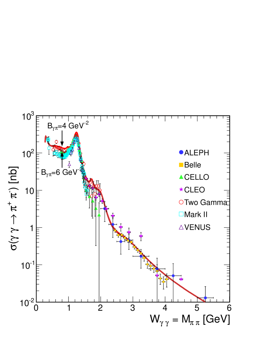
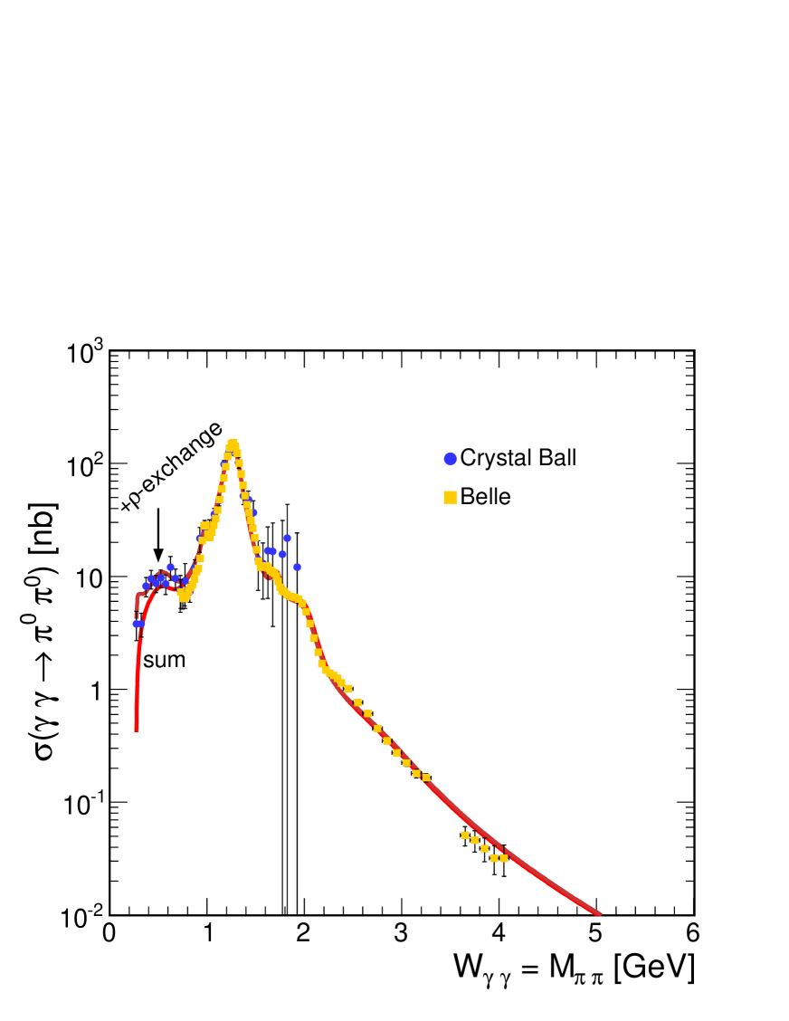
Figure 9: Results of the fit: the total cross section ($\gamma\gamma\to\pi^{+}\pi^{-}$ for $|\cos\theta|<$ 0.6, $\gamma\gamma\to\pi^{0}\pi^{0}$ for $|\cos\theta|<$ 0.8).

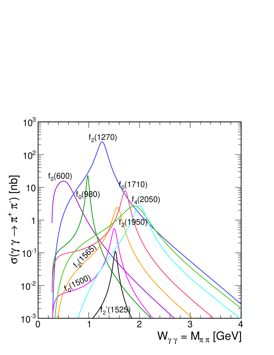
Figure 10: Contributions of different s-channel resonances to the $\gamma\gamma\to\pi^{+}\pi^{-}$ reaction.

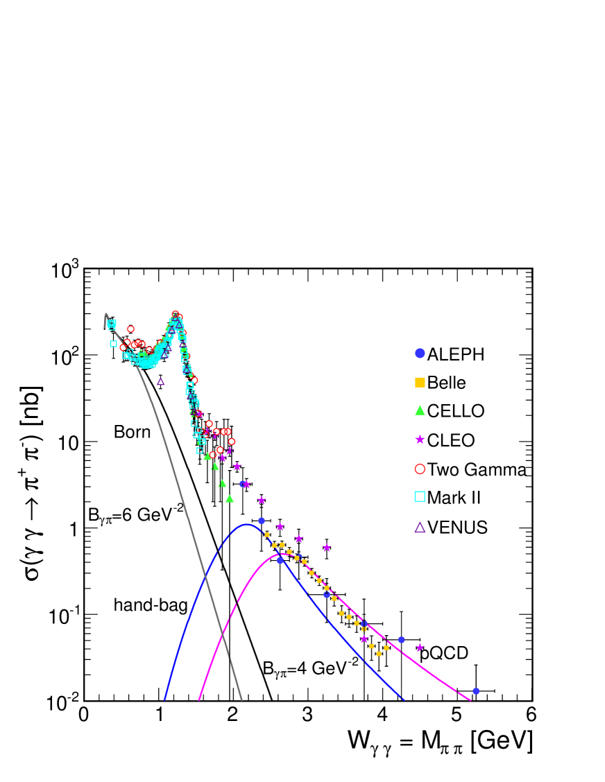
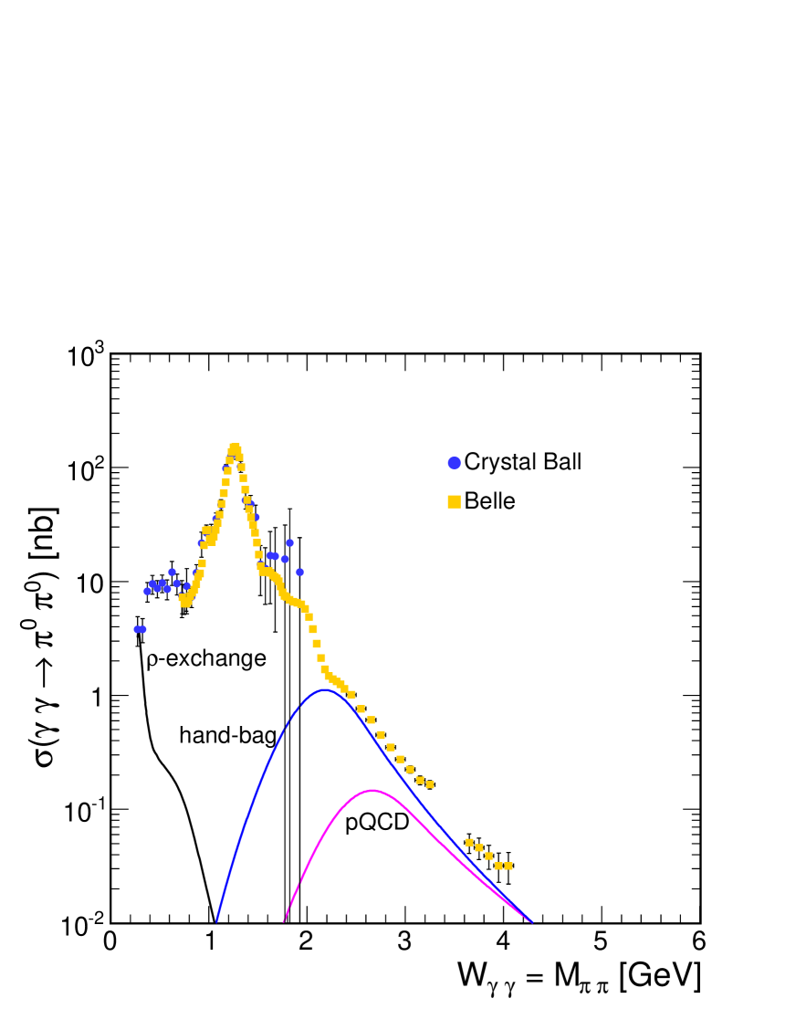
Figure 11: Contributions of different continuum processes. The meaning of the curves is explained in the figures.

We wish to show first cross section for $\gamma\gamma\to\pi^{+}\pi^{-}$ and $\gamma\gamma\to\pi^{0}\pi^{0}$ processes as a function of the subprocess energy. We shall include the pion exchange mechanism for the $\gamma\gamma\to\pi^{+}\pi^{-}$ reaction, several resonance states, pion-pion rescattering important, as will be shown below, for $\gamma\gamma\to\pi^{0}\pi^{0}$ reaction where in the leading order the pion exchange continuum vanishes. At somewhat higher energies we include also the Brodsky-Lepage pQCD and hand-bag mechanisms. In Fig.9 we show our model calculations against world data for $\gamma\gamma\to\pi\pi$ Aleph ; Belle_Mori ; Belle_Nakazawa ; Cello ; Cleo ; Gamma ; Mark_II ; Venus ; Belle_Uehara09 ; Crystal_Ball . We get a good agreement with all available data points for the first time in such a large range of energies. This makes our hybrid model for $\gamma\gamma\to\pi\pi$ well suited for the predictions of the cross sections for nucleus-nucleus collisions.

Our model amplitude is a sum of many ingredients as discussed in the previous section. In Fig.10 and Fig.11 we show some somewhat artificially separated ingredients to the final spectrum. We show s-channel resonance (Fig.10) and continuum (Fig.11) contributions separately. At low energies, the $\sigma(600)$ s-channel resonance as well as pion rescattering due to $\rho$-meson exchange play crucial role. At somewhat higher energies the spectra are dominated by the contribution of the tensor $f_{2}(1270)$ meson. At still higher energies the situation is less clear. The smallness of the cross section at $W\sim$ 1.5 GeV can be understood as an interference of right wing of the tensor $f_{2}(1270)$ resonance and other resonances ($f^{\prime}_{2}(1525)$, $f_{0}(1500)$, $f_{2}(1565)$). At around $W\sim$ 2 GeV, we observe a new irregular behaviour. This can be understood as the presence of s-channel spin-4 contribution. In order to describe the angular distribution we use a simple model assuming that the spin-4 amplitude is proportional to $\mathcal{M}_{\lambda_{1}\lambda_{2}}\sim Y_{4,\lambda_{1}-\lambda_{2}}\delta_{\lambda_{1}-\lambda_{2},}$ (type B). This is similar to what was found from a phenomenological analysis in Ref.Belle_Uehara09 . A much better description of the data is obtained when the $f_{4}(2050)$ resonance is included. The corresponding radiative decay width is treated as a free parameter. We get $\Gamma_{f_{4}\to\gamma\gamma}$ = 0.7 keV $\pm$ 0.1 keV. This is rather a rough estimate than a rigorous statistical analysis. The problem is in the background which is in this range of invariant masses rather difficult to control. Our analysis is a first trial to extract the radiative decay width of the $f_{4}(2050)$ resonance. The found value is much smaller than that for the $f_{2}(1270)$ (3.035 keV) and comparable to that for $f_{0}(980)$ (0.29 keV) (see Table 1). We shall not discuss consequences of better understanding of the structure of $f_{4}(2050)$ resonance. This certainly goes beyond the scope of the present paper.

Clearly, the tensor $f_{2}(1270)$ is the dominant resonance. Other resonances give much smaller but sizeable absolute cross section. However, their separation is not an easy task especially from the analysis of total cross section. As was discussed recently Machado_glueball , the cross section for the production of glueballs (G) in the nucleus-nucleus $AA\to AGA$ reaction could be large. However, selecting a final state is in this context a very important issue. The $\pi\pi$ final state is an obvious candidate. Our analysis shows that searching for glueballs in the $\pi\pi$ channels may be extremely difficult, if not impossible. This makes the heavy ion processes not the best tool to study glueballs or other exotic mesons. We think that a precise fit of the present Belle angular distribution is probably better than any fit to the future nuclear data.

In Fig.11, we show the contributions of the Brodsky-Lepage and hand-bag mechanisms. Please note that our normalization of the hand-bag mechanism was adjusted to describe high-energy experimental data together with the Brodsky-Lepage mechanism. In Ref.HB only the hand-bag mechanism, ignoring the Brodsky-Lepage mechanism, was fitted to the high-energy data. For the $\pi^{+}\pi^{-}$ channel we show in addition the continuum distribution corresponding to pion exchange for two different values of slope parameter and for the $\pi^{0}\pi^{0}$ channel rescattering contribution due to $\rho^{\pm}$ t-channel exchanges. The corresponding contribution falls quickly with increasing energy and plays an important role only up to $W=$ 1 GeV. In Fig.9 (right panel) we show the sum of resonances, BL pQCD and hand-bag mechanisms - lower line. The upper curve includes in addition the $\rho^{\pm}$ exchange contribution. Adding the $\rho$ exchange contribution allows us to better describe experimental data for small invariant masses.

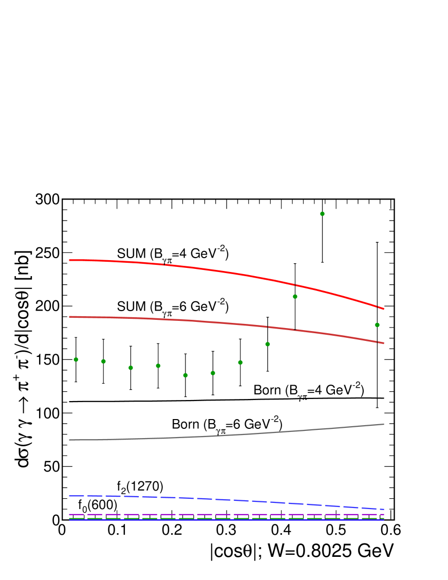
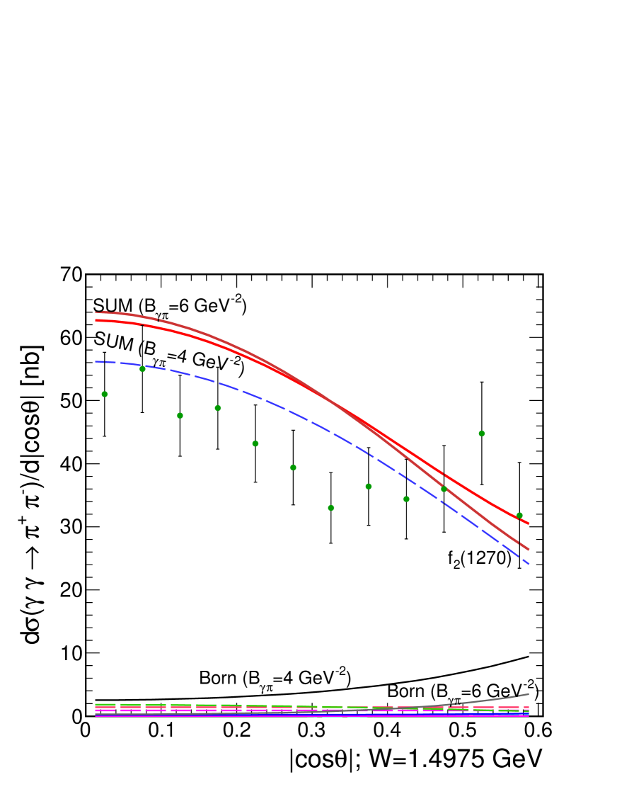
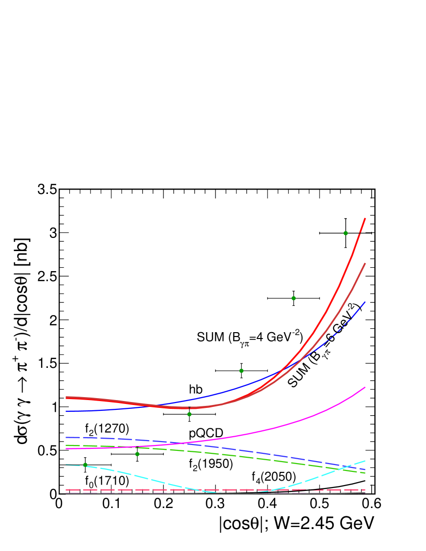
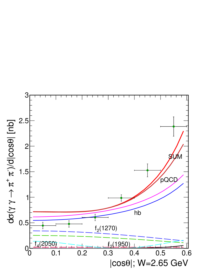
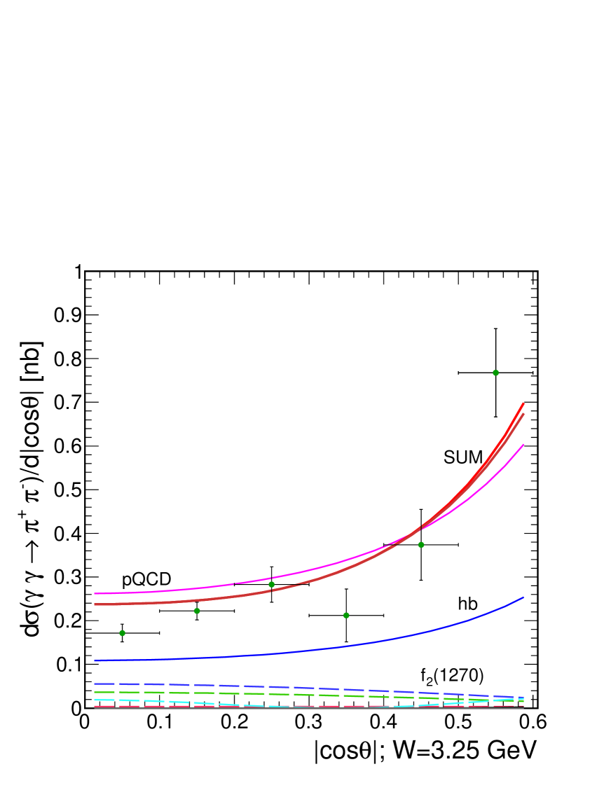
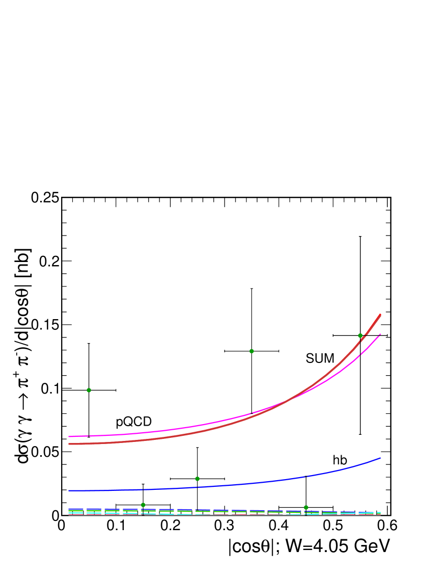
Figure 12: Examples of angular distributions for the $\gamma\gamma\to\pi^{+}\pi^{-}$ reaction.

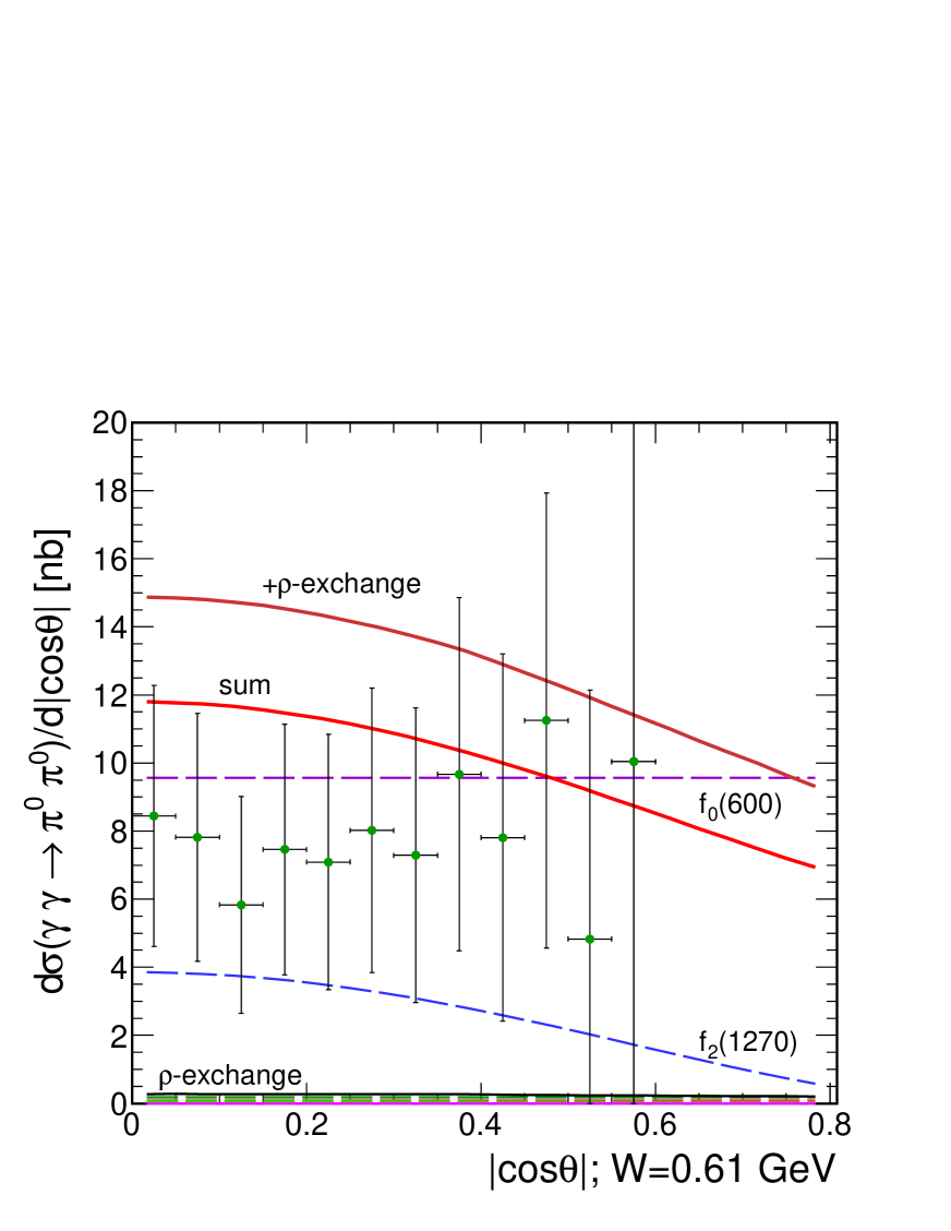
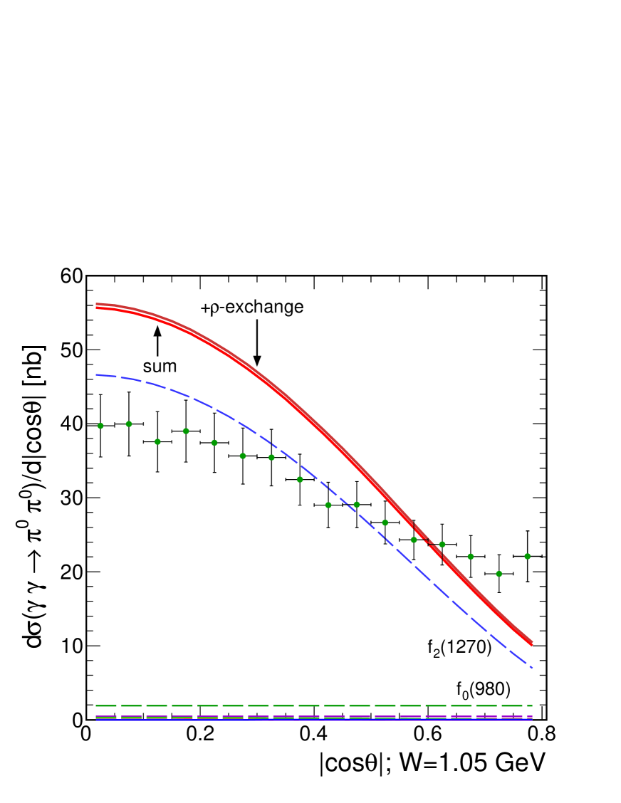
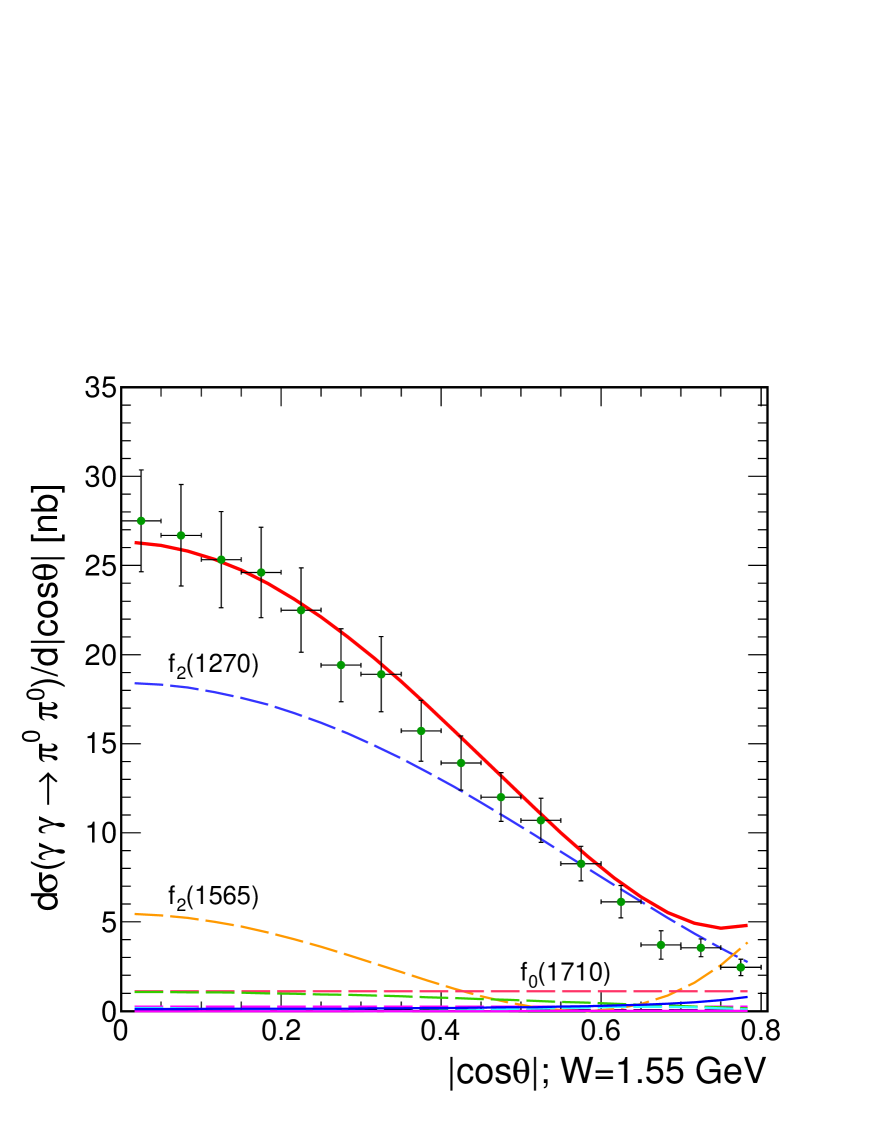
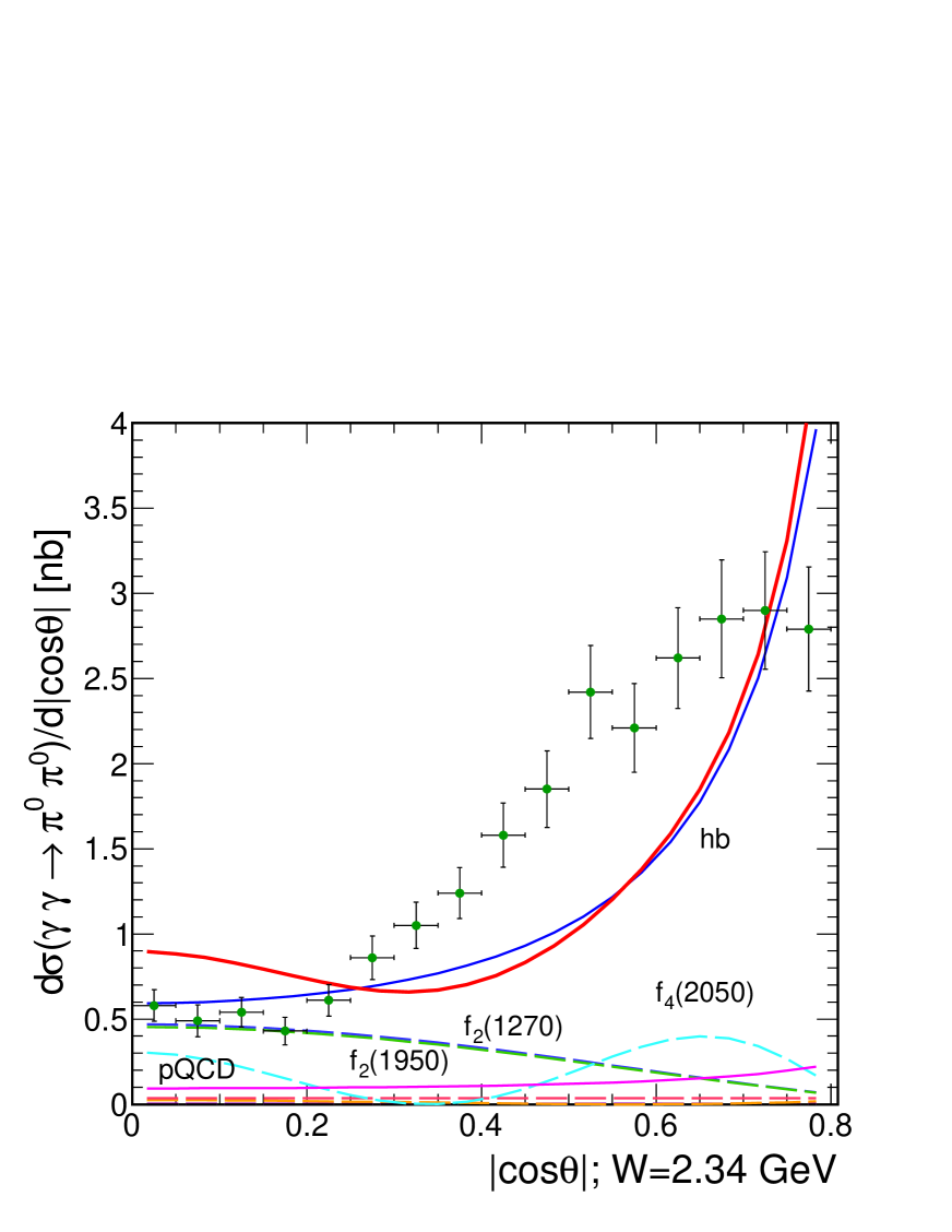
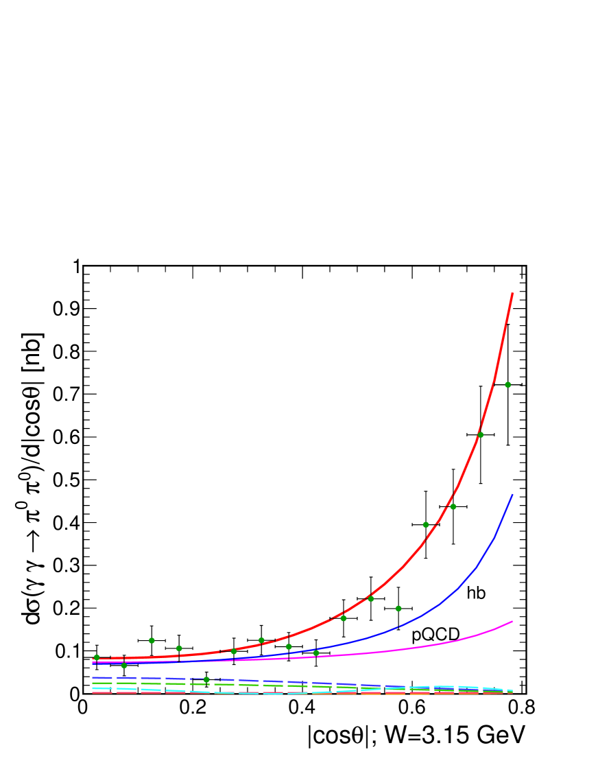
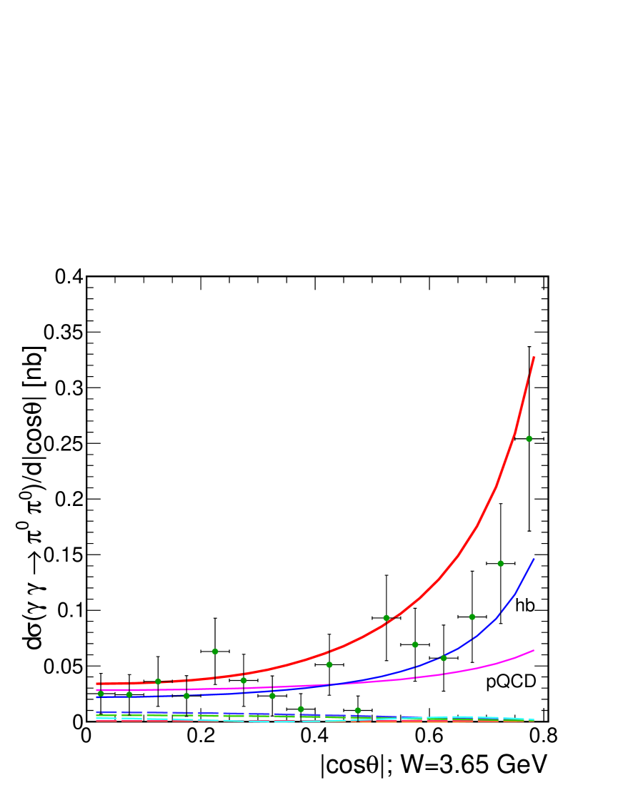
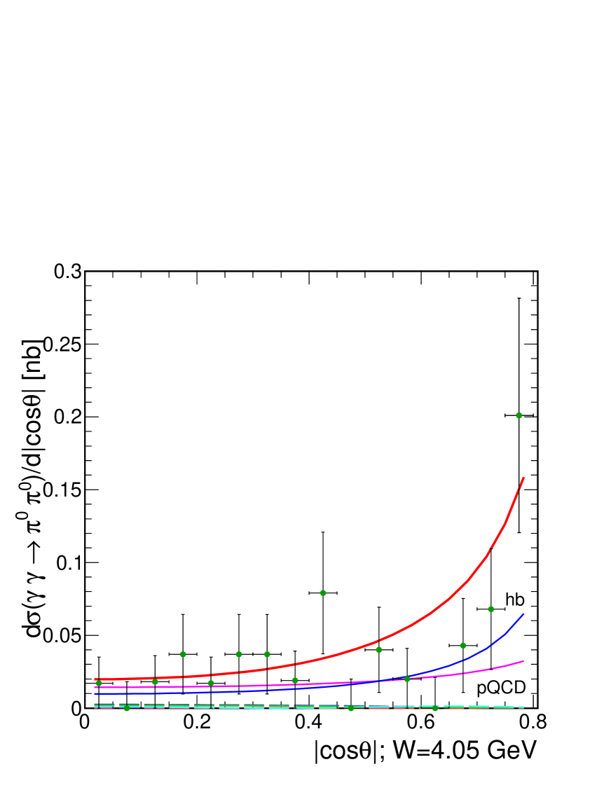
Figure 13: Examples of angular distributions for the $\gamma\gamma\to\pi^{0}\pi^{0}$ reaction.

Figure 14: The ratio of the $\gamma\gamma\to\pi^{0}\pi^{0}$ and $\gamma\gamma\to\pi^{+}\pi^{-}$ cross sections as a function of $W_{\gamma\gamma}=\sqrt{s_{\gamma\gamma}}$.

In Fig.12 and 13 we compare our predictions to the angular experimental data measured by the Belle Collaboration. Experimental data points are taken from Refs. Belle_Mori ; Belle_Nakazawa for $\gamma\gamma\to\pi^{+}\pi^{-}$ and from Ref.Belle_Uehara09 for $\gamma\gamma\to\pi^{0}\pi^{0}$ reactions. In Fig. 12 (the first four panels) we show the sum of contributions of many mechanisms for two different values of the slope parameter in the hadronic form factors (see below Eq. (8)). We show how the final result depends on the value of this parameter. In Ref.SS03 the results for $B<$ 4 GeV^-2 were shown, but here we obtain a better description of the data when we use the exponential form factor with $B_{\gamma\pi}$=6 GeV^-2. The description for $W=$1.4975 GeV shows that one should include also $D$ wave, but we have no theoretical guidance how to do it. For larger $W$, the contribution from pQCD mechanisms starts to dominate. In Fig.13 we show the angular distribution for $\gamma\gamma\to\pi^{0}\pi^{0}$ process for nine different energies ranging from 0.61 GeV to 4.05 GeV. Here we use the same parameters of resonances (masses, widths, phases) as for the $\gamma\gamma\to\pi^{+}\pi^{-}$ reaction. Here we have a small problem with good description for two energies (1.05 and 2.34 GeV). In addition, we show the cross section corresponding to the sum of processes (amplitudes) with and without contribution of the $\rho^{\pm}$-meson exchange. We can observe that the inclusion of this contribution is important only for $W<$ 0.6 GeV (see. Fig.9, right panel). In conclusion, we have obtained a reasonable description of the angular experimental data, which results in excellent description of the total cross section (see Fig.9).

In Fig.14 we present the ratio of the neutral and charged pion pair cross sections. The upper line represents the hand-bag model result, which is independent of $\theta$ and is equal to $\frac{1}{2}$. Our result, which includes the BL pQCD and hand-bag contribution simultaneously, describes the experimental data measured by the Belle Collaboration Belle_Nakazawa ; Belle_Uehara09 . We have a problem with correct description of the data at $W=$ (2.4-2.7) GeV. We think that this is due to not exact description of angular experimental data for $\gamma\gamma\to\pi^{0}\pi^{0}$ reaction in this range of energy. However, our result shows that for the correct description of high energy cross section it is necessary to take into account also the BL pQCD contribution.

In Fig.15 we summarize our elementary cross sections as a function of $\sqrt{s}_{\gamma\gamma}$ and $\cos\theta$. Here transverse momentum cuts were imposed as explained in the figure caption. The lower cut roughly corresponds to the lower cut of the ALICE experiment. It is not clear for us if such a cut is sufficient to regularize the calculations of the BL pQCD and hand-bag mechanisms. Therefore we present also a result with slightly bigger cut. Another option would be to cut in $\cos\theta$ as is usually done at $e^{+}e^{-}$ colliders. The irregularities observed at z $\approx\pm$ 1 are caused by small number of bins in the figure. Such two-dimensional distributions as shown in Fig.15 are then used in nuclear calculations discussed in the next subsection.

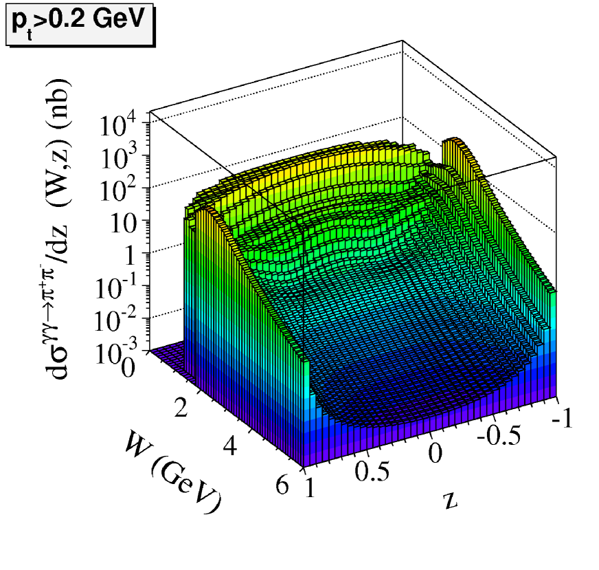
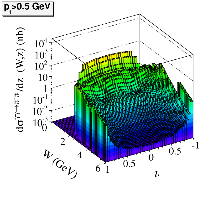
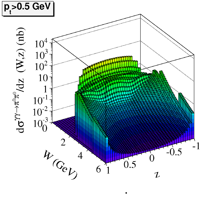
Figure 15: $\frac{d\sigma}{dz}(W,z)$ for $\gamma\gamma\to\pi^{+}\pi^{-}$ (left) and $\gamma\gamma\to\pi^{0}\pi^{0}$ (right) for two different cuts on pion transverse momenta: $p_{t,\pi}>$ 0.2 GeV (top) and $p_{t,\pi}>$ 0.5 GeV (bottom).

III.2 $PbPb\to PbPb\pi\pi$

In order to check our nuclear calculation, in Fig.16 we show interesting distribution in impact parameter between the two lead nuclei. The distribution is different from zero starting from the distance of $b=2R_{A}\approx$ 14 fm and extends till ”infinity”. This means that a big part of the cross section comes from the situations when the two ${}^{208}Pb$ nuclei fly by very far one from each other. This figure clearly demonstrates the ultraperipheral character of the discussed process of exclusive dipion production via photon-photon fusion.

Figure 16: The impact parameter distribution for the $PbPb\to PbPb\pi^{+}\pi^{-}$ and $PbPb\to PbPb\pi^{0}\pi^{0}$ reactions at $\sqrt{s_{NN}}=$ 3.5 TeV.

Table 2: Cross sections for different lower cuts on pion transverse momenta at $\sqrt{s_{NN}}$ = 3.5 TeV.

$p_{t,min}$ [GeV]	$\pi^{+}\pi^{-}$ [mb]	$\pi^{0}\pi^{0}$ [mb]
0.2	46.7	8.7
0.5	12.1	5.1
1.0	0.08	0.05

The total cross sections for $\sqrt{s_{NN}}$ = 3.5 TeV are collected for both $\pi^{+}\pi^{-}$ and $\pi^{0}\pi^{0}$ channels for different lower cuts on pion transverse momentum in Table 2.

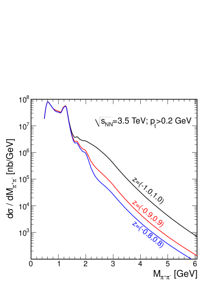
Figure 17: Total cross section for $\gamma\gamma\to\pi^{+}\pi^{-}$ (left panel) and $\gamma\gamma\to\pi^{0}\pi^{0}$ (right panel) as a function of the system energy at the LHC energy $\sqrt{s_{NN}}=$ 3.5 TeV and $p_{t,\pi}>$ 0.2 GeV. We show in addition results with extra cuts on $z$.

The distribution in invariant dipion mass shown in Fig.17 is the most interesting one. We show somewhat theoretical distribution for the full phase space (upper solid line). We show distributions for the $PbPb\to PbPb\pi^{+}\pi^{-}$ (left panel) and for the $PbPb\to PbPb\pi^{0}\pi^{0}$ (right panel) reactions for the full phase space (upper lines), for $|\cos\theta|<$ 0.9 (middle lines) and for the angular range corresponding to the experimental limitations usually used for the $\pi\pi$ production in $e^{+}e^{-}$ collisions ($|\cos\theta|<$ 0.8). At lower energies ($W<$ 1.5 GeV) the result does not depend on the angular cuts. The big differences start in the region where the elementary cross section is described by the BL pQCD and hand-bag mechanisms.

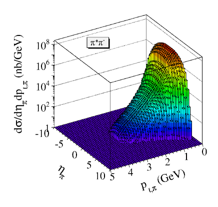
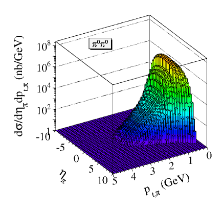
Figure 18: $\frac{d\sigma}{d\eta_{\pi}dp_{t,\pi}}$ for the $\mbox{${}^{208}Pb$}+\mbox{${}^{208}Pb$}\to\mbox{${}^{208}Pb$}\mbox{${}^{208}Pb$}\pi^{+}\pi^{-}$ reaction (left panel) and the $\mbox{${}^{208}Pb$}+\mbox{${}^{208}Pb$}\to\mbox{${}^{208}Pb$}\mbox{${}^{208}Pb$}\pi^{0}\pi^{0}$ reaction (right panel) at the LHC energy $\sqrt{s_{NN}}=$ 3.5 TeV and $p_{t,\pi}>$ 0.2 GeV.

Fig.18 shows two-dimensional distributions in pseudorapidity of charged pion (left panel) or pseudorapidity of neutral pion (right panel) and transverse momentum of one of the pions. With higher $p_{t,\pi}$ values, the pseudorapidity distribution becomes somewhat narrower.

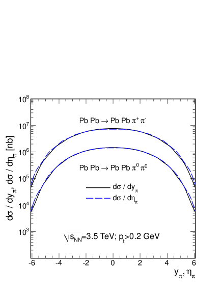
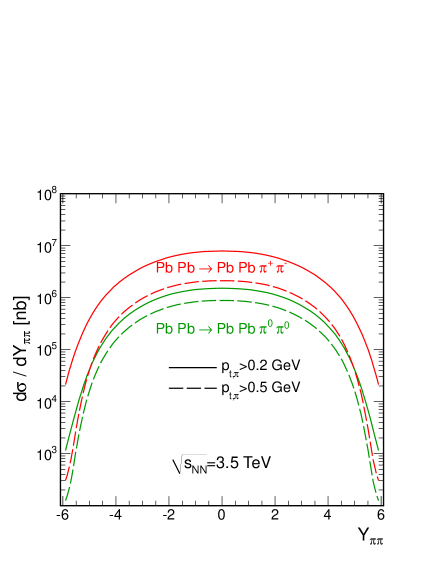
Figure 19: $\frac{d\sigma}{dy_{\pi}}$ and $\frac{d\sigma}{d\eta_{\pi}}$ (left panel) and $\frac{d\sigma}{dY_{\pi\pi}}$ (right panel) for the LHC energy $\sqrt{s_{NN}}=$ 3.5 TeV.

Let us start now presentation of theoretical differential distributions which can be in principle measured. In the left panel of Fig.19 we show distributions in rapidity of individual pions from the pair (solid line) as well as distribution in pseudorapidity of the same pion (dashed line). Right panel illustrates nuclear cross section as the function of the pion pair rapidities. Here we have imposed extra cuts on pion transverse momenta: $p_{t,\pi}>$ 0.2 GeV (solid lines) and $p_{t,\pi}>$ 0.5 GeV (dashed lines). In addition, we compare the nuclear cross section for $\pi^{+}\pi^{-}$ (upper curves) and for $\pi^{0}\pi^{0}$ (lower curves) production. These distributions (in $y_{\pi}$, $\eta_{\pi}$ and $Y_{\pi\pi}$) look fairly similar.

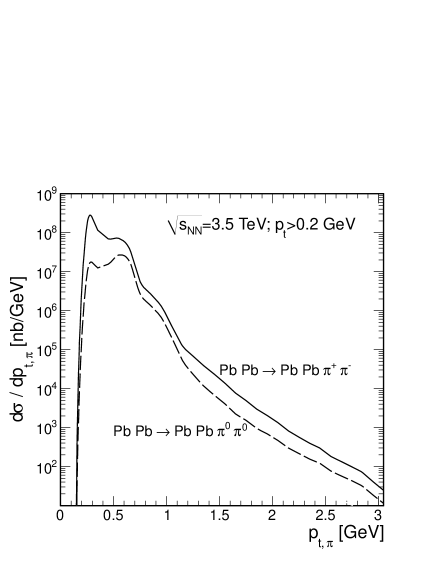
Figure 20: $\frac{d\sigma}{dp_{t}}$ of one of pions for the LHC energy $\sqrt{s_{NN}}=$ 3.5 TeV and $p_{t,\pi}>$ 0.2 GeV.

The distribution in transverse momentum of one of the pions is shown in Fig. 20 for the full phase space for $PbPb\to PbPb\pi^{+}\pi^{-}$ (solid line) and for $PbPb\to PbPb\pi^{0}\pi^{0}$ (dashed line), respectively. The distribution shown in Fig.20 is for the full range of (pseudo)rapidities. The ALICE detector can cover only a part of the whole rapidity range.

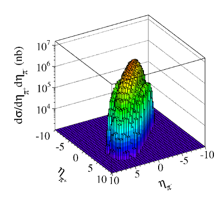
Figure 21: $\frac{d\sigma}{d\eta_{\pi^{+}}d\eta_{\pi^{-}}}$ for the $\mbox{${}^{208}Pb$}+\mbox{${}^{208}Pb$}\to\mbox{${}^{208}Pb$}\mbox{${}^{208}Pb$}\pi^{+}\pi^{-}$ reaction at the LHC energy $\sqrt{s_{NN}}=$ 3.5 TeV and $p_{t,\pi}>$ 0.2 GeV.

In Fig.21 we show a two-dimensional distribution of pseudorapidities of pions. The cross section is concentrated along the diagonal $\eta_{1}=\eta_{2}$. The range covered by the ALICE detector (a square (-0.9,0.9)$\times$(-0.9,0.9) centered around $\eta_{1}$ = $\eta_{2}$ = 0) is rather small. The pseudorapidity distribution of one of the pions is shown in Fig.19 (left panel) by the dashed line.

III.3 $\rho^{0}(770)$ and $\rho^{0}(1450)$ photoproduction in PbPb collisions

The $\pi^{+}\pi^{-}$ pairs produced in ultraperipheral photon-photon (sub)collisions constitutes a background for, e.g., exclusive production of the $\rho^{0}$ meson. This reaction was studied experimentally at RHIC rho0_RHIC . Theoretical calculations for LHC energies predict very large cross section of the order of a few barns (see e.g. KN99 ; FSZ ; GM11 ; RSZ2011 ), i.e., more than two orders of magnitude larger than the contribution of the mechanism discussed here (see also Table 3). The $\rho^{0}$ spectrum is, however, concentrated in pion-pion invariant mass around the $\rho$-resonance position. It is an open question how far from the resonance position one can trust a rather naive Breit-Wigner form. In photoproduction of $\rho^{0}$ meson on protons one often fits the following form:

$$\frac{d\sigma(PbPb\to PbPb\rho^{0})}{dM_{\pi\pi}}=\left|A_{\rho^{0}}\frac{\sqrt{M_{\pi\pi}m_{\rho^{0}}\Gamma(M_{\pi\pi})}}{M_{\pi\pi}^{2}-m_{\rho^{0}}^{2}+im_{\rho^{0}}\Gamma(M_{\pi\pi})}+A_{\pi\pi}\right|^{2}\;,$$ (43)

where $A_{\rho^{0}}$ is the amplitude for the Breit–Wigner function, $A_{\pi\pi}$ is the amplitude for the direct $\pi^{+}\pi^{-}$ production and $\Gamma(M_{\pi\pi})$ is the momentum-dependent width of the $\rho^{0}$ resonance. In our presentation below the values of parameters are taken from Ref.rho_STAR and the integrated total cross section was assumed to be 5 barn (see Table 3).

Table 3: Cross sections for coherent $\rho$ and $\rho^{\prime}$ production for LHC.

Reference/model	$\sqrt{s_{NN}}$ [TeV]	$\sigma_{tot}^{\rho^{0}(770)}$ [b]	$\sigma_{tot}^{\rho^{0}(1450)}$ [b]
KN KN99	5.6	5.2
FSZ FSZ	5.5	9.538	2.216
RSZ RSZ2011	5.5	9.706
IKS IKS /KST-R	5.5	4.9
/KST		4.36
/GBW		3.99
/VDM		10.03
GM GM	5.5	10.069

In Fig.22 we show the contribution of the $\rho^{0}(770)$ meson integrated over the whole phase space, without any extra cuts. While the predictions for the $\rho^{0}$ production are rather uncertain (within factor two or three), our predictions for the $\gamma\gamma$ process should be fairly precise (a few percent precision). A comparison with real data should be therefore interesting. At larger dipion invariant masses, other radial excitation may appear in addition. The $\rho^{0}(1450)$ state is a first candidate of this type. Since the continuum single-photon photoproduction $\pi^{+}\pi^{-}$ background in this region was not studied, we have no information about its interference with the $\rho^{0}(1450)$ resonance. Therefore in the following we shall show only the resonance contribution and leave the question of the background for future analyses, including perhaps the ALICE experimental data. Here we parametrize the $\rho^{0}(1450)$ contribution as:

$$\frac{d\sigma(PbPb\to PbPb\rho^{0}(1450))}{dM_{\pi\pi}}=\left|A_{\rho^{0}(1450)}\frac{\sqrt{M_{\pi\pi}m_{\rho^{0}(1450)}\Gamma(M_{\pi\pi})}}{M_{\pi\pi}^{2}-m_{\rho^{0}(1450)}^{2}+im_{\rho^{0}(1450)}\Gamma(M_{\pi\pi})}\right|^{2}\;.$$ (44)

The cross section for the photoproduction of $\rho^{0}(1450)$ was calculated only in Ref.FSZ . This calculation finds that the cross section for the $\rho^{0}(1450)$ resonance is about a factor 5 smaller than for $\rho^{0}(770)$. Here we are discussing the signal in the $\pi^{+}\pi^{-}$ channel, therefore a corresponding branching fraction has to be included in addition. Unfortunately this branching fraction is not well known. The Crystal Ball Collaboration has measured only the ratio of the cross section for two and four pion channels Crys_Barrel . They have found $Br(2\pi)/Br(4\pi)$ = 0.37 $\pm$ 0.1. In this situation we can only calculate an upper limit for the two-pion branching fraction:

$$Br\left(\rho^{0}(1450)\to\pi^{+}\pi^{-}\right)=\frac{P_{2\pi}}{P_{2\pi}+P_{4\pi}+P_{other}}<\frac{P_{2\pi}}{P_{2\pi}+P_{4\pi}}=\frac{P_{2\pi}/P_{4\pi}}{P_{2\pi}/P_{4\pi}+1}\approx 0.27\;.$$ (45)

Figure 22: Invariant mass distribution of $\pi^{+}\pi^{-}$ from the decay of $\rho^{0}(770)$ and $\rho^{0}(1450)$ photo-production (resonance contributions represented by the dashed and dotted lines) and our $\gamma\gamma$ fusion (solid line) in ultraperipheral Pb-Pb collisions at $\sqrt{s_{NN}}=$ 3.5 TeV.

In Fig.22 the resonance contribution for the $\rho^{0}(1450)$ is 5/0.27 times smaller than for $\rho^{0}(770)$ as suggested by the calculation FSZ and the above upper limit for the branching fraction into pions. It is therefore clear that this will be an upper estimate for the $\rho^{0}(1450)$ contribution. The relative contribution of $\rho^{0}(1450)$ is still somewhat larger than observed for instance in the electroproduction of these states at HERA ZEUS . In Ref.NNZ94 an anomalous (strongly nucleus mass and photon virtuality dependent) production of $\rho^{0}(1450)$ has been predicted for incoherent production in the $\gamma^{*}A\to\rho^{0}(1450)X$ reaction. We wish to emphasize in addition that our estimate does not take into account experimental cuts of any concrete experiment.

The photoproduction contribution cross sections are above our photon-photon fusion one. It is not clear in the moment how the kinematical cuts may change the proportions of the two mechanisms. This will be studied elsewhere.

In contrast, the $PbPb\to PbPb\pi^{0}\pi^{0}$ reaction is free of the photoproduction mechanisms. However, it is not clear for us if, in this case, a measurement is possible.

IV Conclusions

In the present paper we have discussed first $\gamma\gamma\to\pi^{0}\pi^{0}$ and $\gamma\gamma\to\pi^{+}\pi^{-}$ reactions and we have shown that different mechanisms contribute to such processes below $\sqrt{s_{\gamma\gamma}}<$ 6 GeV.

These are: pion exchange for the $\pi^{+}\pi^{-}$ channel, several resonances such as $f_{0}(600)$, $f_{0}(980)$, $f_{2}(1270)$, $f_{0}(1500)$, $f^{\prime}_{2}(1525)$, $f_{2}(1565)$, $f_{0}(1710)$, $f_{2}(1950)$ and $f_{4}(2050)$ and pQCD mechanisms proposed first by Brodsky and Lepage as well as hand-bag mechanism proposed by Diehl, Kroll and Vogt. We have included also pion-pion rescattering which leads to a coupling between the $\pi^{+}\pi^{-}$ and $\pi^{0}\pi^{0}$ channels. We have shown that the inclusion of such processes can help in understanding energy dependence of the $\gamma\gamma\to\pi\pi$ processes as well as angular distributions only at very low energies. We have not tried to get a perfect fit to the data as several details of the model amplitudes are not known. We have slightly adjusted some parameters to get a reasonable description of the data.

We have found that the decay width $\sigma(600)\to\gamma\gamma$ is much smaller than that found in other partial wave analyses. The data (total cross section as well as angular distributions) close to the position of $f_{2}(1270)$ peak can be described assuming the dominance of the amplitude

${\cal M}_{\lambda_{1}\lambda_{2}}^{f_{2}(1270)}\propto Y_{2,\lambda_{1}-\lambda_{2}}(\theta,\phi)\cdot\left(\delta_{\lambda_{1}-\lambda_{2},-2}+\delta_{\lambda_{1}-\lambda_{2},2}\right)$ .

We have included also the tensor $f_{2}(1565)$ resonance, considering two models of the corresponding $\gamma\gamma\to\pi\pi$ amplitude. A better description of the data has been obtained using

${\cal M}_{\lambda_{1}\lambda_{2}}^{f_{2}(1565)}\propto Y_{2,\lambda_{1}-\lambda_{2}}(\theta,\phi)\cdot\delta_{\lambda_{1}-\lambda_{2},0}$ ,

i.e., space, different than for $f_{2}(1270)$. This may mean that the structure of this resonance is completely different than that for $f_{2}(1270)$, $f^{\prime}_{2}(1525)$ or $f_{2}(1950)$ ($q\bar{q}$ states).

Inclusion of the $f_{4}(2050)$ spin-4 resonance improves the spectrum and angular distributions around the resonance position. By fitting to the Belle Collaboration data we have found $\Gamma_{f_{4}(2050)\to\gamma\gamma}$ = 0.7 $\pm$ 0.1 keV.

At still higher energies the situation is even less clear. While in the $\pi^{+}\pi^{-}$ channel the Brodsky-Lepage mechanism with distribution amplitude discussed recently in the context of the BABAR data describes the data, in the ”smaller” $\pi^{0}\pi^{0}$ channel more processes may contributed in addition to the BL pQCD mechanism. Another possibility is the hand-bag mechanism proposed some time ago by Diehl, Kroll and Vogt. The hand-bag mechanism may be important only at energies $W>$ 3 GeV.

At high energies the angular distributions show an enhancement at large $|\cos\theta|$ for the $\gamma\gamma\to\pi^{0}\pi^{0}$. Such an enhancement is predicted both, by the Brodsky-Lepage and by the hand-bag approaches. A proper mixture of both processes provides a better description of the experimental data than each of them separately, as done usually in the literature.

Having fixed the details of the amplitude we have calculated total cross sections and angular distribution as a function of $\gamma\gamma$ energy for both $\gamma\gamma\to\pi^{+}\pi^{-}$ and $\gamma\gamma\to\pi^{0}\pi^{0}$ processes. These two subprocess energy-dependent cross sections have been used next in Equivalent Photon Approximation in the impact parameter space to calculate for the first time corresponding production rate in ultraperipheral ultrarelativistic heavy ion reactions. In this calculation we have taken into account realistic charge distributions in colliding nuclei.

We have calculated both total cross sections at LHC energy, as well as distributions in rapidity and transverse momentum of pions and dipion invariant mass. The calculation of distributions of individual pions is slightly more complicated in the b-space EPA. The distributions in dipion invariant mass have been compared with the contribution of exclusive $\rho^{0}\to\pi^{+}\pi^{-}$ production in photon-pomeron (pomeron-photon) mechanism taken from the literature. Close to the $\rho^{0}$ resonance the $\gamma\gamma\to\pi^{+}\pi^{-}$ mechanism yields only a small contribution. The $\gamma\gamma$ contribution could be, perhaps, measured outside of the $\rho^{0}$ resonance window. A detailed comparison with the absolutely normalized ALICE experimental data should allow a quantitative test of our predictions. Imposing several experimental cuts may enhance the $\gamma\gamma\to\pi\pi$ contribution.

In the present paper we have analysed exclusive production of two pions. In principle exclusive production of four pions could be also interesting. First experimental study has been presented in rho0_RHIC . Interesting theoretical study has been performed in PSSW2008 .

Appendix A A comment on partial wave decomposition

In our model, the amplitude for the $\gamma\gamma\to\pi\pi$ process is a coherent sum of different contributions (amplitudes) for different mechanisms:

$${\cal M}_{\lambda_{1},\lambda_{2}}(W)=\sum_{k}{\cal M}^{(k)}_{\lambda_{1},\lambda_{2}}(W)\;,$$ (46)

where $\lambda_{1}$, $\lambda_{2}$ are initial photon helicities. There are only four combinations of helicities defining the, in general, complex amplitude: (-1,1),(1,-1),(1,1),(-1,-1).

As a consequence the differential distributions for the $\gamma\gamma\to\pi\pi$ reaction can be written in terms of spherical harmonics numbered with pion-pion angular momentum projection ($M=\lambda_{1}-\lambda_{2}$)

$$\frac{d\sigma}{d\Omega} = |C_{0,0}(W)Y_{0,0}(z,\phi)+C_{2,0}(W)Y_{2,0}(z,\phi)+C_{4,0}(W)Y_{4,0}(z,\phi)+(...)|^{2}$$ (47)

$$+ |C_{2,2}(W)Y_{2,2}(z,\phi)+C_{4,2}(W)Y_{4,2}(z,\phi)+(...)|^{2}$$

$$+ |C_{2,-2}(W)Y_{2,-2}(z,\phi)+C_{4,-2}(W)Y_{4,-2}(z,\phi)+(...)|^{2}\;.$$

The expansion coefficients $C_{L,M}$ are strongly energy dependent. In general, resonance contributions (L = 0, 2, 4) interfere with slowly-energy-dependent backgrounds (L = 0, 2, 4,…) of different origin discussed in previous sections.

Recently the Belle Collaboration Belle_Uehara09 ; Belle_Uehara08 has performed a simplified fit to the experimental angular distributions of the type:

$$\frac{d\sigma}{d\Omega} = |C_{0,0}(W)Y_{0,0}(z)|^{2}+|C_{2,0}(W)Y_{2,0}(z)|^{2}+|C_{4,0}Y_{4,0}(z)|^{2}$$ (48)

$$+ |C_{2,2}(W)Y_{2,2}(z)|^{2}+|C_{4,2}(W)Y_{4,2}(z)|^{2}\;.$$

Our model shows that such a simplified partial wave expansion has not always model justification and may therefore lead sometimes to unphysical solutions. However, the correct partial wave decomposition (see (Eq.47)) of experimental angular distributions is in practice too difficult, if not impossible.

Acknoweledgments

We are indebted to Nikolai Achasov and Wolfgang Schäfer for interesting exchange of informations and Christoph Mayer for a discussion of ALICE experiment and exchange of a few experimental details as well as careful reading of our manuscript. This work was partially supported by the Polish grant N N202 078735, N N202 236640 and DEC-2011/01/B/ST2/04535. A big part of the calculations within this analysis was carried out with the help of cloud computer system (Cracow Cloud One) of Institute of Nuclear Physics (PAN).

References

• (1) V.M. Budnev, I.F. Ginzburg, G.V. Meledin and V.G. Serbo, Phys. Rep. 15 (1975) 4; C.A.Β Bertulani and G. Baur, Phys. Rep. 163 (1988) 29; G. Baur, K. Hencken, D. Trautmann, S.Β Sadovsky, and Y. Kharlov, Phys. Rep. 364 (2002) 359; A.J. Baltz, G. Baur, D.Β d’Enterria et al., Phys. Rep. 458 (2008) 1.
• (2) R. Engel, A. Schiller and V.G. Serbo, Z. Phys. C71 (1996) 651; U.D. Jentschura and V.G.Β Serbo, Eur. Phys. J. C64 (2009) 309.
• (3) M. KΕ‚usek-Gawenda and A. Szczurek, Phys. Rev. C82 (2010) 014904.
• (4) G. Baur and L. G. Ferreira Filho, Nucl. Phys. A518 (1990) 786.
• (5) M. KΕ‚usek, A. Szczurek, and W. SchΓ€fer, Phys. Lett. B674 (2009) 92.
• (6) M. KΕ‚usek-Gawenda, A. Szczurek, M. V. T. Machado an d V. G. Serbo, Phys. Rev. C83 (2011) 024903.
• (7) M. Łuszczak and A. Szczurek, Phys. Lett. B700 (2011) 116.
• (8) M. KΕ‚usek-Gawenda and A. Szczurek, Phys. Lett. B700 (2011) 322.
• (9) J. Bijnens and F. Cornet, Nucl. Phys. B296 (1988) 557; J. F. Donoghue, B. R. Holstein and Y. C. Lin, Phys. Rev. D37 (1988) 2423; J. F. Donoghue and B. R. Holstein, Phys. Rev. D48 (1993) 137; S. Bellucci, J. Gasser and M. E. Sainio, Nucl. Phys. B423 (1994) 80; J. A.Β Oller and E. Oset, Nucl. Phys. A629 (1998) 739; L. V. Fil’kov and V. L. Kashevarov, Phys. Rev. C72 (2005) 035211; J. Gasser, M. A. Ivanov, M. E. Sainio, Nucl.Phys. B745 (2006) 84; J.Β A.Β Oller and L. Roca, Eur. Phys. J. A37 (2008) 15; L. V. Fil’kov and V. L. Kashevarov, Phys. Rev. C81 (2010) 029801; I. V. Danilkin, M. F. M. Lutz, S. Leupold and C. Terschlusen, arXiv: 1211.1503 [hep-ph].
• (10) N.N. Achasov and G.N.Β Shestakov, JETP Lett. 88 (2008) 295; N.N. Achasov and G.N.Β Shestakov, Uspekhi Fizicheskih Nauk 181 (2011) 827 (arXiv: 0905.2017 [hep-ph]).
• (11) N. N. Achasov and G. N. Shestakov, Phys. Rev. D77 (2008) 074020.
• (12) P. Ko, Phys. Rev. D41 (1990) 1531.
• (13) G. Mennessier, S. Narison and X.-G. Wang, Nucl. Phys. Proc. Suppl. 207: (2010) 177.
• (14) M. R. Penninhton, T. Mori, S. Uehara and Y. Watanabe, Eur. Phys. J. C56 (2008) 1; M.Β Boglione and M. R. Pennington, Eur. Phys. J. C9 (1999) 11.
• (15) V. L. Chernyak, Phys. Lett. B640 (2006) 246.
• (16) A. Szczurek and J. Speth, Nucl. Phys. A728 (2003) 182.
• (17) S. J. Brodsky and G. P. Lepage, Phys. Rev. D24 (1981) 1808.
• (18) C. R. Ji and F. Amiri, Phys. Rev. D42 (1990) 3764.
• (19) M. Diehl, P. Kroll and C. Vogt, Phys. Lett. B532 (2002) 99; M. Diehl and P. Kroll, Phys. Lett. B683 (2010) 165.
• (20) Aleph Collaboration (R. Barate et al.), Phys. Lett. B472 (2000) 189.
• (21) M. V. T. Machado and M. L. L. da Silva, Phys. Rev. C83 (2011) 014907.
• (22) Belle Collaboration (S. Uehara et al.), Phys. Rev. D79 (2009) 052009.
• (23) B. Grube, Nucl. Phys. Proc. Suppl. 179 (2008) 117.
• (24) A. J. Baltz, S. R. Klein and J. Nystrand, Phys. Rev. Lett. 89 (2002) 012301.
• (25) L. Frankfurt, M. Strikman and M. Zhalov, Phys. Rev. C67 (2003) 034901.
• (26) S. Brodsky, T. Kinoshita and H. Terazawa, Phys. Rev. D4 (1971) 1532.
• (27) M. Poppe, Int. J. Mod. Phys. A1 (1986) 545.
• (28) K. Nakamura et al. (Particle Data Group), J. Phys. G37 (2010) 075021.
• (29) Belle Collaboration (S. Uehara et al.), Phys. Rev. D78 (2008) 052004.
• (30) JADE Collaboration (T. Oest et al.), Z. Phys. C47 (1990) 343.
• (31) J. M. Blatt and V. Weisskopf, Theoretical Nuclear Physics, John Wiley, New York, 1952.
• (32) Crystal Barrel Collaboration (C.A. Baker et al.), Phys. Lett. B467 (1999) 147.
• (33) V.A. Schegelsky, A.V. Sarantsev, V.A. Nikonov and A.V. Anisovich, Eur. Phys. J. A27 (2006) 207.
• (34) Belle Collaboration (T. Mori et al.), J. Phys. Soc. Jap. 76 (2007) 074102.
• (35) A.V. Efremov and A.V. Radyushkin, Phys. Lett. B94 (1980) 245.
• (36) S.J. Brodsky and G.P. Lepage, Phys. Lett. B87 (1979) 359.
• (37) D. MΓΌller, Phys. Rev. D51 (1995) 3855.
• (38) E.R. Arriola and W. Broniowski, Phys. Rev. D66 (2002) 094016.
• (39) X.G. Wu and T. Huang, Phys. Rev. D82 (2010) 034024.
• (40) BABAR Collaboration, B. Aubert, et al., Phys.Rev. D80 (2009) 052002.
• (41) Belle Collaboration (H. Nakazawa et al.), Phys. Lett. B615 (2005) 39.
• (42) R. Hagedorn, Relativistic Kinematics, High Energy Physics: W.A. Benjamin, Inc. Reading Massachusetts 1963.
• (43) S. Klein and J. Nystrand, Phys. Rev. C60 (1999) 014903.
• (44) L. Frankfurt, M. Strikman and M. Zhalov, Phys. Lett. B537 (2002) 51.
• (45) L. Frankfurt, M. Strikman and M. Zhalov, Phys. Lett. B537 (2002) 51; Phys. Rev. C67 (2003) 034901.
• (46) V. Rebyakova, M. Strikman and M. Zhalov, Phys. Lett. B710 (2012) 647.
• (47) V.P. Goncalves and M.V.T. Machado, Phys. Rev. C84 (2011) 011902.
• (48) A. Cisek, W. SchΓ€fer and A. Szczurek, Phys. Rev. C86 (2012) 014905.
• (49) C.A. Bertulani, S.R. Klein and J. Nystrand, Ann. Rev. Nucl. Part. Sci. 55 (2005) 271.
• (50) Crystal Ball Collaboration (H. Marsiske et al.), Phys. Rev. D41 (1990) 3324.
• (51) ALEPH Collaboration (A. Heister et al.), Phys. Lett. B569 (2003) 140.
• (52) CELLO Collaboration (H.J. Behrend et al.), Z. Phys. C56 (1992) 381.
• (53) CLEO Collaboration (J. Dominick et al.), Phys. Rev. D50 (1994) 3027.
• (54) Two Gamma Collaboration (H. Aihara et al.), Phys. Rev. Lett. 57 (1986) 404.
• (55) Mark II Collaboration (J. Boyer et al.), Phys. Rev. D42 (1990) 1350.
• (56) VENUS Collaboration (F. Yabuki et al.), J. Phys. Soc. Jap. 64 (1995) 435.
• (57) B. Grube, Nucl. Phys. B (Proc. Suppl.) 179 (2008) 117; STAR Collaboration (B.I. Abelev et al.), Phys. Rev. C81 (2010) 044901.
• (58) STAR Collaboration (B.I. Abelev et al.), Phys. Rev. C77 (2008) 034910; STAR Collaboration (G. Agakishiev et al.), Phys. Rev. C85 (2012) 014910.
• (59) CB-ELSA Collaboration (A. Abele et al.), Eur. Phys. J. C21 (2001) 261
• (60) ZEUS Collaboration (H. Abramowicz et al.), Eur. Phys. J. C72 (2012) 1869.
• (61) J. Nemchik, N.N. Nikolaev and B.G. Zakharov, Phys. Lett. B339 (1994) 194.
• (62) Y. Ivanov, B. Kopeliovich and I. Schmidt, arXiv: 0706.1532 [hep-ph] (CERN Workshop Heavy Ion Collisions at the LHC).
• (63) V.P. Goncalves and M.V.T. Machado, J. Phys. G32 (2006) 295.
• (64) B. Pire, F. Schwennsen, L. Szymanowski and S. Wallon, Phys. Rev. D78 (2008) 094009.