Generation of magnetic fields in Einstein-Aether gravity

Abstract

Recently the lower bounds of the intergalactic magnetic fields $10^{-16}\sim 10^{-20}$ Gauss are set by gamma-ray observations while it is unlikely to generate such large scale magnetic fields through astrophysical processes. It is known that large scale magnetic fields could be generated if there exist cosmological vector mode perturbations in the primordial plasma. The vector mode, however, has only a decaying solution in General Relativity if the plasma consists of perfect fluids. In order to investigate a possible mechanism of magnetogenesis in the primordial plasma, here we consider cosmological perturbations in the Einstein-Aether gravity model, in which the aether field can act as a new source of vector metric perturbations. The vector metric perturbations induce the velocity difference between baryons and photons which then generate magnetic fields. This velocity difference arises from effects at the second order in the tight-coupling approximation. We estimate the angular power spectra of temperature and B-mode polarization of the Cosmic Microwave Background (CMB) Anisotropies in this model and put a rough constraint on the aether field parameters from latest observations. We then estimate the power spectrum of associated magnetic fields around the recombination epoch within this limit. It is found that the spectrum has a characteristic peak at $k=0.1h{\rm Mpc^{-1}}$, and at that scale the amplitude can be as large as $B\sim 10^{-22}$ Gauss where the upper bound comes from CMB temperature anisotropies. The magnetic fields with this amplitude can be seeds of large scale magnetic fields observed today if the sufficient dynamo mechanism takes place. Analytic interpretation for the power spectra is also given.

I Introduction

Astronomical observations have shown that magnetic fields exist ubiquitous in various astrophysical objects, ranging from planets to clusters of galaxies or even larger systems Giovannini (2004); Widrow (2002); Ryu et al. (2012). On large scales such as in galaxies and clusters of galaxies, measurements of the Faraday rotation indicate that the strength of magnetic fields is about $\sim 10^{-6}$ Gauss. Recently the lower bounds of the intergalactic magnetic field are found as $10^{-16}\sim 10^{-20}$ Gauss Neronov and Vovk (2010); Pandey and Sethi (2013), depending on the data used and assumptions they have made.

The origin of such large scale magnetic fields remains as an enigma and much effort has been made to explain the origin in a wide variety of ways. It is believed that the magnetic fields in galaxies can be amplified and maintained by the dynamo mechanism, which is a hydro-magnetic process with magnetic reconnections (e.g. refs. Widrow (2002); Widrow et al. (2012)). However, we still need a seed field for the dynamo process to act on. To explain the observed magnetic fields in galaxies in the present universe, the seed field should be as large as $10^{-20}\sim 10^{-30}$ Gauss at kpc comoving scale Davis et al. (1999). It is an interesting scenario that such small seed fields may end up with the intergalactic magnetic fields of $\gtrsim 10^{-20}$ Gauss due to adiabatic compression.

The seed magnetic fields are possible to originate from quantum fluctuations of the electro-magnetic fields stretched by inflation in the early universe. If the conformal invariance is broken by some mechanisms during the inflation era Martin and Yokoyama (2008); Subramanian (2010); Demozzi et al. (2009); Kanno et al. (2009), magnetic fields with a large coherence length can be naturally generated beyond the horizon scale. In this case, however, there are associated nagging problems, namely, the back reaction and the strong coupling problems. The former is that inflation fails to proceed if the generated electromagnetic fields dominate the energy density in the universe during inflation. The latter problem is related with the naturalness of the model building. Due to these problems, there is no satisfactory model so far to explain observed magnetic fields Fujita and Mukohyama (2012). Nevertheless, the effects of primordial magnetic fields on the present observations have been well investigated Fujita and Mukohyama (2012); Paoletti and Finelli (2012); Yamazaki et al. (2012); Fedeli and Moscardini (2012). Another possible mechanism to generate seed magnetic fields is the phase transition in the early universe (e.g. ref. Widrow et al. (2012)). Phase transition releases the free energy as a latent heat with forming bubbles, and the bubble collisions can generate electric current and hence magnetic fields. However, the magnetic fields generated at the phase transition generally have small coherence length which corresponds to the Hubble radius at the transition. In this case, therefore, inverse cascading processes of magnetic fields are necessary to explain the ones at large scales.

On the other hand, some astrophysical processes may become natural candidates of the origin of the seed magnetic fields. For example, the Biermann battery Biermann and Schlüter (1951), which is effective in non-adiabatic situations such as shocks, can generate magnetic fields in starts Kemp (1982), supernova shocks Hanayama et al. (2005); Miranda et al. (1998), large scale structure formation Kulsrud et al. (1997), and cosmological reionizatoin Gnedin et al. (2000). However, since the mechanism works effectively only in places where the matter or astronomical objects are present, it may be difficult to explain the existence of the intergalactic magnetic fields if they are in void regions Takahashi et al. (in preparation.).

In this paper, we consider yet another mechanism to generate the seed magnetic fields, i.e., the vorticity in the primordial plasma before the recombination epoch Harrison (1970). Because photons push electrons more frequently than ions through Thomson scatterings, the vorticity in the photon fluid can induce circular current and thus generate magnetic fields. The problem here is that in a Friedmann universe with perfect fluids, the solution of the vorticity has only a decaying mode. In order to have nonzero vorticity, some mechanisms are proposed, which include the free-streaming neutrinos Lewis (2004); Ichiki et al. (2012), the cosmological defects Hollenstein et al. (2008), and the nonlinear couplings of the first order density perturbations Ichiki et al. (2012); Takahashi et al. (2005); Fenu et al. (2011).

Following this idea, here we show that a possible modification of gravity, namely the Einstein-Aether gravity Jacobson and Mattingly (2001), can also generate nonzero vorticity and thus magnetic fields. The Einstein-Aether gravity is known as a healthy extension of Hořava-Lifshits gravity at low energies Jacobson (2010); Blas et al. (2010), which originally proposed by Hořava Horava (2009a, b) as a candidate of the theory of quantum gravity. The Einstein-Aether gravity contains a new regular vector degree of freedom which is called “the aether field”. Effects of the aether field have been discussed intensively, for example, in connection with the inflation era and late-time accelerating expansion of the universe Zlosnik et al. (2008); Zuntz et al. (2010); Meng and Du (2012); Barrow (2012), Cosmic Microwave Background radiation (CMB) temperature anisotropies Lim (2005); Zuntz et al. (2008, 2010) and compact objects Eling et al. (2007); Garfinkle et al. (2007); Eling and Jacobson (2006). The purpose of this paper is to examine the role of the vorticity excited by the aether field in the generation of magnetic fields before the recombination epoch.

The plan of this paper is as follows. In section II, we review the Einstein-Aether gravity and describe a formalism of the vector-mode perturbations. In section III, we focus on the evolution equation of magnetic fields in the primordial plasma. In section IV, we explore the evolution of the aether field and perturbations. Our main results will be described in this section. Section V is devoted to our summary. In Appendix A, we summarize the observational and theoretical constraints on the aether parameters. In Appendix B, we formulate cosmological perturbations in the Einstein-Aether gravity and define the scalar-vector-tensor decomposition.

Throughout this paper, we use the units in which $c=\hbar=1$ and the metric signature as $(-,+,+,+)$. We obey the rule that the subscripts and superscripts of the Greek characters and alphabets run from 0 to 3 and from 1 to 3, respectively.

II Einstein-Aether gravity

In this section, we summarize the Einstein-Aether gravity. The action for the Einstein-Aether gravity is given by Jacobson and Mattingly (2001)

$$S=\frac{1}{16\pi G}\int{d^{4}x\sqrt{-g}\left[R+\mathcal{L}_{A}\right]}+\int{d^{4}x\sqrt{-g}\mathcal{L}_{m}}\ ,$$ (1)

where $\mathcal{L}_{A}$ is written in the form:

$$\mathcal{L}_{A}=K+\lambda(A^{\alpha}A_{\alpha}+1)\ ,$$ (2)

$$K\equiv K^{\alpha\beta}_{\ \ \mu\nu}\left(\nabla_{\alpha}A^{\mu}\right)\left(\nabla_{\beta}A^{\nu}\right)\ ,$$ (3)

$$K^{\alpha\beta}_{\ \ \mu\nu}\equiv c_{1}g^{\alpha\beta}g_{\mu\nu}+c_{2}\delta^{\alpha}_{\ \mu}\delta^{\beta}_{\ \nu}+c_{3}\delta^{\alpha}_{\ \nu}\delta^{\beta}_{\ \mu}-c_{4}A^{\alpha}A^{\beta}g_{\mu\nu}\ .$$ (4)

Here, $\mathcal{L}_{m}$ is the Lagrangian of the ordinary matter, $R$ is the Ricci scalar, and $\mathcal{L}_{A}$ is the Lagrangian of the aether field $A_{\mu}$. We assume that the aether field does not couple to the matter. The constant $G$ is different from Newton’s gravitational constant which is locally measured. That is to say, $G$ is a “bare” parameter. We will see that $G$ is renormalized. The coefficients $c_{1},\ c_{2},\ c_{3}$ and $c_{4}$ are the set of parameters of the Einstein-Aether gravity. These parameters are constrained by observations and theoretical hypotheses as summarized in Appendix A. This theory contains a massive ghost Armendariz-Picon and Diez-Tejedor (2009), and one usually imposes a fixed-norm constraint on the vector to remove such a ghost. This is equivalent to forcing a Lorentz-breaking on the vacuum expectation value. The parameter $\lambda$ is a Lagrange multiplier to fix the norm.

To derive a set of equations of motions, we take variations with respect to variables. Variation with respect to the Lagrange multiplier $\lambda$ imposes the condition that

$$A^{\mu}A_{\mu}=-1\ .$$ (5)

This equation is the constraint equation of the aether field $A^{\mu}$. Owing to the fixed norm, we will eliminate the possibility that the degree of residual freedom acts as a ghost Armendariz-Picon et al. (2010).

Variation with respect to the aether field $A^{\mu}$ gives the equation of motion and the continuous equation for the aether field as

$$\nabla_{\alpha}J^{\alpha}_{\ \ \mu}+c_{4}A^{\alpha}\left(\nabla_{\alpha}A^{\gamma}\right)\left(\nabla_{\mu}A_{\gamma}\right)=\lambda A_{\mu}\ ,$$ (6)

where we define $J^{\alpha}_{\ \ \mu}$ as

$$\begin{split}J^{\alpha}_{\ \ \mu}&\equiv K^{\alpha\beta}_{\ \ \mu\nu}\nabla_{\beta}A^{\nu}\\ &=c_{1}\nabla^{\alpha}A_{\mu}+c_{2}\delta^{\alpha}_{\ \mu}\nabla_{\beta}A^{\beta}+c_{3}\nabla_{\mu}A^{\alpha}-c_{4}A^{\alpha}A^{\beta}\nabla_{\beta}A_{\mu}\ .\end{split}$$ (7)

Variation with respect to the metric $g^{\mu\nu}$ gives the Einstein equation with the aether field,

$$R_{\mu\nu}-\frac{1}{2}Rg_{\mu\nu}=T^{(A)}_{\mu\nu}+8\pi GT^{(M)}_{\mu\nu}\ ,$$ (8)

where we also define energy momentum tensors $T^{(A)}_{\mu\nu}$ and $T^{(M)}_{\mu\nu}$ as

$$\begin{split}&T^{(A)}_{\mu\nu}\equiv-\frac{1}{\sqrt{-g}}\frac{\delta(\sqrt{-g}\mathcal{L}_{A})}{\delta g^{\mu\nu}}\ ,\\ &T^{(M)}_{\mu\nu}\equiv-\frac{2}{\sqrt{-g}}\frac{\delta(\sqrt{-g}\mathcal{L}_{M})}{\delta g^{\mu\nu}}\ .\end{split}$$ (9)

Note that the factors of the energy momentum tensors for the aether field and the matter are different. The concrete expression of $T^{(A)}_{\mu\nu}$ can be written as

$$T^{(A)}_{\mu\nu}=\nabla_{\sigma}\left(\mathcal{I}^{\sigma}_{\ \mu\nu}\right)+\mathcal{Y}^{(c_{1})}_{\mu\nu}-\mathcal{Z}^{(c_{4})}_{\mu\nu}+\lambda A_{\mu}A_{\nu}+\frac{1}{2}g_{\mu\nu}\mathcal{L}_{A}\ .$$ (10)

Here we define the tensors $\mathcal{I}^{\sigma}_{\ \mu\nu}$, $\mathcal{Y}^{(c_{1})}_{\mu\nu}$ and $\mathcal{Z}^{(c_{4})}_{\mu\nu}$ as

$$\begin{split}\mathcal{Z}^{(c_{4})}_{\mu\nu}&\equiv c_{4}A^{\alpha}A^{\beta}\left(\nabla_{\alpha}A_{\mu}\right)\left(\nabla_{\beta}A_{\nu}\right)\ ,\\ \mathcal{Y}^{(c_{1})}_{\mu\nu}&\equiv c_{1}\left(\nabla^{\sigma}A_{\mu}\nabla_{\sigma}A_{\nu}-\nabla_{\mu}A^{\sigma}\nabla_{\nu}A_{\sigma}\right)\ ,\\ \mathcal{I}^{\sigma}_{\ \mu\nu}&\equiv A_{(\mu}J^{\ \ \sigma}_{\nu)}-A_{(\mu}J^{\sigma}_{\ \ \nu)}-A^{\sigma}J_{(\mu\nu)}\ ,\end{split}$$ (11)

where the parentheses, _(μν), mean symmetrization. For convenience we use the abbreviations, which are written in the forms:

$$\begin{split}\alpha&=c_{1}+3c_{2}+c_{3}\ ,\\ c_{123}&=c_{1}+c_{2}+c_{3}\ ,\\ c_{13}&=c_{1}+c_{3}\ ,\\ c_{14}&=c_{1}+c_{4}\ .\end{split}$$ (12)

Because theoretical parameters have four independent components, we will treat $\alpha,c_{14},c_{13}$ and $c_{1}$ as the independent model parameters.

II.1 Background cosmology

In this subsection, we explore background cosmology where the space-time is given by a spatially flat Friedmann-Robertson-Walker metric. The line element is given by

$$ds^{2}=a^{2}(\eta)[-d\eta^{2}+d{\bf x}^{2}]\ .$$ (13)

From Eq. (5), the background components of the vector $A^{\mu}$ are given by

$$A^{\mu}=\left(a^{-1},0,0,0\right)\ .$$ (14)

Substituting Eq. (14) into Eq. (6), the $\mu=0$ component of Eq. (6) can be written as

$$\lambda=\frac{3}{a^{2}}\left(c_{123}\mathcal{H}^{2}-c_{2}\mathcal{\dot{H}}\right)\ ,$$ (15)

where $\mathcal{H}=\dot{a}/a$, and a dot represents a derivative with respect to the conformal time $\eta$. Similarly we substitute Eqs. (13) and (14) into Eq. (8), and we derive the Friedmann equations with the aether field as

$$\begin{split}\mathcal{H}^{2}&=\frac{8\pi G_{\rm cos}}{3}a^{2}\rho\ ,\\ \mathcal{\dot{H}}&=-\frac{4\pi G_{\rm cos}}{3}a^{2}(\rho+3p)\ .\end{split}$$ (16)

Here we define $G_{\rm cos}=\frac{G}{1-\alpha/2}$, and $\rho$ and $p$ are the energy density and pressure of the ordinary matter, respectively. The effect of the aether field can only be seen in the renormalization of Newton’s gravitational constant in the background cosmology.

In the Newtonian limit which should be applied to laboratory measurements, the Einstein equation can be rewritten in the form of the Poisson equation Carroll and Lim (2004) as

$$\nabla^{2}\Phi=4\pi G_{\rm N}\rho_{m}\ ,$$ (17)

where $G_{\rm N}=\frac{G}{1+c_{14}/2}$. Because $G_{\rm cos}$ and $G_{\rm N}$ can be different, the ratio of $G_{\rm cos}$ and $G_{\rm N}$ is constrained by observations such as the light element abundance from the Big-Bang Nucleosynthesis (BBN) Carroll and Lim (2004) (see Appendix A). From that we have a constraint on the aether parameters as $c_{14}+\alpha\lesssim 0.2$. We assume that $c_{14}=-\alpha$ in this paper for simplicity, which leads to $G_{\rm cos}=G_{\rm N}$.

II.2 Vector-mode perturbations

In this subsection, we consider cosmological perturbations in the Einstein-Aether gravity (see also Appendix B). Since we are interested in generation of magnetic fields via the vector-mode perturbations, we focus on the vector-mode in this paper, and we omit indices ^(±1) or ^(v) that represent the vector-mode in Appendix B. The scalar-vector-tensor decomposition is also defined in Appendix B. We will work in the synchronous gauge in which the metric is given by

$$ds^{2}=a^{2}\left[-d\eta^{2}+\left(\delta_{ij}+h_{ij}\right)dx^{i}dx^{j}\right]\ ,$$ (18)

where $h_{ij}$ is the metric perturbation. Under this metric, the aether field can be expressed in the form as

$$\begin{split}A^{\mu}&=\left(\frac{1}{a},\frac{V^{i}}{a}\right)\ ,\\ A_{\mu}&=\left(-a,aV_{i}\right)\ ,\end{split}$$ (19)

where we have imposed $A^{\mu}A_{\mu}=-1$. Raising or lowering indices of $V_{i}$ is done by $\delta_{ij}$. Substituting the above equations into Eqs. (8) and (6), we derive the evolution equations of the perturbed quantities. The equation of motion for the aether field is given by

$$c_{14}\left(\ddot{V}+2\mathcal{H}\dot{V}\right)-(\alpha-c_{14})\mathcal{\dot{H}}V+(\alpha+c_{14})\mathcal{H}^{2}V+c_{1}k^{2}V+\frac{1}{2}c_{13}k^{2}\sigma=0\ .$$ (20)

The Einstein equations for the vector mode are given by

$$\dot{\sigma}+2\mathcal{H}\sigma=-\frac{c_{13}}{1+c_{13}}\left(\dot{V}+2\mathcal{H}V\right)-\frac{16\pi Ga^{2}p\pi}{(1+c_{13})k}\ ,$$ (21)

$$k^{2}\sigma=\frac{1}{1+c_{13}}\left[16\pi Ga^{2}q-c_{13}k^{2}V\right]\ ,$$ (22)

where $\sigma\equiv\dot{h}^{(\pm 1)}/k$ denotes the shear and $h^{(\pm 1)}$ are the metric perturbations of the vector mode defined in Appendix B, and $p\pi$ and $q$ denote the anisotropic stress and the heat flux of the ordinary matter, respectively.

To see the behavior of the aether field, we solve Eq. (20) without the ordinary matter contribution on $\sigma$ first. The ordinary matter is subdominant in the evolution of the vector perturbations in the Einstein-Aether gravity, although we will include the matter contributions correctly in our numerical calculations. This is because the ordinary matter does not couple to the aether field while the aether field and the metric couple directly. Thus the aether field can amplify predominantly the metric perturbation as its source, namely, Eq. (22) can be rewritten as

$$\sigma\simeq-\frac{c_{13}}{1+c_{13}}V\ .$$ (23)

This assumption is justified by the initial conditions and the numerical results. Using Eqs. (20) and (23), we can obtain the evolution equation of the aether field in the closed form as

$$\ddot{V}+2\mathcal{H}\dot{V}+\left[\left(1+\frac{\alpha}{c_{14}}\right)\mathcal{H}^{2}+\left(1-\frac{\alpha}{c_{14}}\right)\dot{H}\right]V+c^{2}_{v}k^{2}V=0\ ,$$ (24)

where $c_{v}$ is the (effective) sound speed of aether field perturbation and defined by

$$c^{2}_{v}\equiv\frac{1}{c_{14}}\left(c_{1}-\frac{1}{2}\frac{c_{13}^{2}}{1+c_{13}}\right)\ .$$ (25)

As a consequence of the existence of the sound speed, the aether field will have a characteristic scale i.e., the “sound horizon” , which is defined as $k_{\rm SH}\equiv aH/c_{v}$. Depending on whether the mode is inside or outside the sound horizon, the behavior of the aether field will change.

When we assume a long-wavelength limit $c_{v}k\eta\ll 1$ in the radiation dominated era (RD) and the matter dominated era (MD), the solutions are given by

$$V(k,\eta)\propto\begin{cases}(k\eta)^{\nu_{\rm rad}}&{\rm RD}\\ (k\eta)^{\nu_{\rm mat}}&{\rm MD}\ ,\\ \end{cases}$$ (26)

where $\nu_{\rm rad}$ and $\nu_{\rm mat}$ are defined by

$$\begin{split}\nu_{\rm rad}&\equiv\frac{-1+\sqrt{1-8\alpha/c_{14}}}{2}\ ,\\ \nu_{\rm mat}&\equiv\frac{-3+\sqrt{1-24\alpha/c_{14}}}{2}\ .\end{split}$$ (27)

These results show that the aether field has the power-law dependence on $k\eta$ outside the sound horizon. Because we are interested in a non-decaying regular mode in the radiation dominated era, we assume that $\alpha/c_{14}\leq 0$. Taking into account the parameter constraint from Eq. (67), the power-law indices, $\nu_{\rm rad}$ and $\nu_{\rm mat}$, must be satisfied with the conditions $0\leq\nu_{\rm rad}\leq 1$ and $-1\leq\nu_{\rm mat}\leq 1$.

Next, we assume the short-wavelength limit $c_{v}k\eta\gg 1$. In this limit, the solutions are given by

$$V(k,\eta)\propto\begin{cases}e^{ic_{v}k\eta}/(k\eta)&{\rm RD}\\ e^{ic_{v}k\eta}/(k\eta)^{2}&{\rm MD}\ .\\ \end{cases}$$ (28)

Both in the radiation and matter dominated eras, the aether field decays as $\propto a^{-1}$ with oscillations.

III magnetic fields generation

In this section, let us consider the generation of magnetic fields. We follow Ref. Ichiki et al. (2012) to formulate the generation process. When there exists the difference of velocities between baryons and photons, magnetic fields can be generated Ichiki et al. (2012); Takahashi et al. (2005); Ichiki et al. (2006); Maeda et al. (2009); Fenu et al. (2011). This is caused by the difference of the Thomson cross sections between electrons and protons. In other words photons push electrons more frequently than protons. As a consequence, the charge separation appears. Photon’s bulk pressure creates the charge separation which induces electric fields, and then magnetic fields will be generated as well. The evolution equation of magnetic fields is derived by the combination of the Maxwell equations and Euler equations for electrons and protons with Thomson scattering Ichiki et al. (2012). It is written in the form:

$$\frac{d\left(a^{2}B^{i}\right)}{dt}=\frac{4\sigma_{T}\rho_{\gamma}a}{3e}\epsilon^{ijk}\partial_{k}\left(v_{\gamma j}-v_{bj}\right)\ ,$$ (29)

where $\sigma_{T}$ is the Thomson cross section and $\epsilon^{ijk}$ is the Levi-Civita symbol and $\rho_{\gamma}$ is the energy density of photons and $v_{\gamma}$ or $v_{b}$ are the velocity of photons or baryons. When we consider scalar perturbations for the velocity fields, the right-hand side of the above equation should vanish. In this paper, we solve the above equation with an initial condition $B=0$ at $z=10^{9}$, which roughly corresponds to the time of neutrino decoupling. By integrating the above equation, the square of the magnetic fields is given by

$$a^{4}B^{i}({\bf k},t)B^{*}_{i}({\bf k^{\prime}},t)=\left(\frac{4\sigma_{T}}{3e}\right)^{2}\left(\delta^{j\ell}\delta^{km}-\delta^{jm}\delta^{k\ell}\right)k_{k}k^{\prime}_{m}\int^{t}_{0}\int^{t}_{0}{a(t^{\prime})\rho_{\gamma}(t^{\prime})\delta v_{j}({\bf k},t^{\prime})a(t^{\prime\prime})\rho_{\gamma}(t^{\prime\prime})\delta v^{*}_{\ell}({\bf k^{\prime}},t^{\prime\prime})dt^{\prime}dt^{\prime\prime}}\ ,$$ (30)

where $\delta v_{j}({\bf k},t^{\prime})\equiv v_{\gamma j}({\bf k},t^{\prime})-v_{bj}({\bf k},t^{\prime})$. Because the evolution equations for baryons, photons and the vector-metric perturbations are independent of $\hat{k}$, we can decompose the vector-mode of the velocity difference between baryons and photons as

$$\delta v({\bf k},t)=V_{\rm ini}({\bf k})\delta v(k,t)~{},$$ (31)

where $V_{\rm ini}({\bf k})$ is the stochastic initial amplitude of the aether field and $\delta v(k,t)$ is the transfer function of the velocity difference between baryons and photons, which is the solution with $V_{\rm ini}=1$. In our calculations, we will relate the initial amplitude $V_{\rm ini}$ to the initial amplitude of the aether field.

By taking an ensemble average and defining the power spectrum, we obtain

$$\Braket{\delta v_{j}({\bf k},t^{\prime})\delta v^{*}_{\ell}({\bf k^{\prime}},t^{\prime\prime})}=(2\pi)^{3}\frac{2\pi^{2}}{k^{3}}\mathcal{P}_{V}(k)P_{j\ell}(\hat{k})\delta v(k,t^{\prime})\delta v(k,t^{\prime\prime})\delta^{3}({\bf k}-{\bf k^{\prime}})\ ,$$ (32)

$$P_{j\ell}(\hat{k})\equiv\delta_{j\ell}-\hat{k}_{j}\hat{k}_{\ell}\ ,$$ (33)

where $\mathcal{P}_{V}(k)$ is the spectrum of the aether field perturbation, which is defined by

$$\Braket{V_{\rm ini}({\bf k})V^{*}_{\rm ini}({\bf k^{\prime}})}\equiv(2\pi)^{3}\frac{2\pi^{2}}{k^{3}}{\mathcal{P}}_{V}(k)\delta({\bf k}-{\bf k^{\prime}})~{}.$$ (34)

Because the parity is not violating in the Einstein-Aether gravity, two helicity states $\lambda=\pm 1$ should not mix. Thus we already omit the superscript ^(λ) here. The power spectrum of magnetic fields is defined as

$$\Braket{B^{i}({\bf k},t)B^{*}_{i}({\bf k^{\prime}},t)}\equiv(2\pi)^{3}S_{B}(k,t)\delta^{3}({\bf k}-{\bf k^{\prime}})\ .$$ (35)

Then we can express $S_{B}(k,t)$ by the initial power spectrum for the aether field $\mathcal{P}_{V}(k)$ as

$$a^{4}(t)\frac{k^{3}}{2\pi^{2}}S_{B}(k,t)=\left(\frac{4\sigma_{T}}{3e}\right)^{2}2\mathcal{P}_{V}(k)k^{2}\left[\int^{t}_{0}{dt^{\prime}a(t^{\prime})\rho_{\gamma}(t^{\prime})\delta v(k,t^{\prime})}\right]^{2}\ .$$ (36)

The initial power spectrum may depend on the inflation model considered. Generally, the initial power spectrum is assumed to be given by a power law as

$$\mathcal{P}_{V}(k)=\mathcal{A}_{V}\left(\frac{k}{k_{0}}\right)^{n_{v}}\ ,$$ (37)

where $k_{0}=0.002{\rm Mpc^{-1}}$ . If we fix the inflation model and the subsequent reheating model, the initial amplitude $\mathcal{A}_{V}$ and spectral index $n_{v}$ can be expressed as a function of the aether parameters and inflation model parameters (see Appendix B).

The amplitude of velocity difference between baryons and photons to generate magnetic fields is dependent on the amplitude of the metric perturbation of the vector-mode. The aether field induces the metric perturbation of the vector-mode dominantly, and therefore the evolution of the aether field is closely related to that of the magnetic fields and their power spectrum.

To understand the behavior of the vector-mode velocities in the presence of aether field, we solve the Euler equation of the baryons for vector-mode. The vector-mode evolution equation for baryons is given by Lewis (2004),

$$\dot{v}_{b}+\mathcal{H}v_{b}=-\frac{4\rho_{\gamma}}{3\rho_{b}}an_{e}\sigma_{T}(v_{b}-v_{\gamma})\ ,$$ (38)

where $n_{e}$ is the electron number density. For photons, we perform a multipole expansion of the Boltzmann equation of photons for the vector-mode as Lewis (2004)

$$\begin{split}&\dot{v}_{\gamma}+\frac{1}{8}k\pi_{\gamma}=-an_{e}\sigma_{T}(v_{\gamma}-v_{b})\ ,\\ &\dot{\pi}_{\gamma}+\frac{8}{5}kI_{3}-\frac{8}{5}kv_{\gamma}=-an_{e}\sigma_{T}\left(\frac{9}{10}\pi_{\gamma}-\frac{9}{5}E_{2}\right)-\frac{8}{5}k\sigma\ ,\\ &\dot{I}_{\ell}+k\frac{\ell}{2\ell+1}\left(\frac{\ell+2}{\ell+1}I_{\ell+1}-I_{\ell-1}\right)=-an_{e}\sigma_{T}I_{\ell}\ ,\end{split}$$ (39)

where $I_{\ell}$ is the $\ell$th order moment of the photon distribution function and $E_{\ell}$ is the $\ell$th order moment of E-mode polarization. The aether field does not affect the Boltzmann equation for photons and the Euler equation for baryons. However the aether field may change the initial conditions for the matter part because the Einstein equation contains the aether field.

Before moving to our numerical calculations, we summarize the initial conditions and the set of equations under the tight-coupling approximation. The initial conditions with the aether field have been derived by assuming that the universe is deep in the radiation dominated era and expanding the equations in powers of $k\eta$ up to the lowest order Nakashima and Kobayashi (2011). Because we are interested in the effects of the aether field, we ignore the regular vector-mode in the presence of the neutrino anisotropic stress which is investigated in Ichiki et al. (2012). Then the aether field in powers of $k\eta$ up to the lowest order is given by

$$V=V_{\rm ini}\eta^{\nu_{\rm rad}}\left[1-\left(1-\frac{\nu_{\rm rad}}{2}\right)\frac{\omega\eta}{4}\right]\ ,$$ (40)

where $\omega=\Omega_{m}\mathcal{H}_{0}/\sqrt{\Omega_{R}}$ and $\Omega_{i}$ are ordinary cosmological density parameters. The initial conditions for the other variables are given by

$$\begin{split}v_{\gamma}&=0\ ,\\ v_{\nu}&=0\ ,\\ \sigma&=-\frac{\nu^{*}_{\rm rad}}{\nu^{*}_{\rm rad}+4R^{*}_{\nu}}\frac{c_{13}}{1+c_{13}}V_{\rm ini}\eta^{\nu_{\rm rad}}\ ,\\ \frac{\pi_{\nu}}{\rho_{\nu}}&=-\frac{8}{15(1+\nu_{\rm rad})}\frac{\nu^{*}_{\rm rad}}{\nu^{*}_{\rm rad}+4R^{*}_{\nu}}\frac{c_{13}}{1+c_{13}}V_{\rm ini}k\eta^{1+\nu_{\rm rad}}\ ,\end{split}$$ (41)

where $R^{*}_{\nu}=(1-\alpha/2)/(1+c_{13})R_{\nu}$, $R_{\nu}=\Omega_{\nu}/\Omega_{r}$, $\nu^{*}_{\rm rad}=5(1+\nu_{\rm rad})(2+\nu_{\rm rad})/2$. We apply these initial conditions to our numerical calculations. In our numerical calculation, we set $V_{\rm ini}=1$ and multiply the power spectrum $P_{V}(k)$ when we derive the variance of the perturbation variables as in Eq. (34).

Deep in the radiation dominated era, photons and baryons frequently interact with each other. These fluids are tightly coupled because the opacity $\dot{\tau}=an_{e}\sigma_{T}$ is large. Hence the tight-coupling parameter $\epsilon$ allows us to expand the equations. The tight-coupling parameter can be expressed as

$$\epsilon=\frac{k}{\dot{\tau}}\sim 10^{-2}\left(\frac{k}{1{\rm Mpc^{-1}}}\right)\left(\frac{1+z}{10^{4}}\right)^{-2}\left(\frac{\Omega_{b}h^{2}}{0.02}\right)^{-1}\ ,$$ (42)

where $\Omega_{b}$ is the baryon density normalized by the critical density and $h\equiv H_{0}/100\;(\rm{km\;s^{-1}\;Mpc^{-1}})$ is the normalized Hubble parameter with $H_{0}$ being the Hubble constant. We expand the equations using the tight-coupling parameter up to second order Ichiki et al. (2012). From here, we quickly review the derivation of expanded equations using the tight-coupling parameter up to the second order. At the zeroth order, Eqs. (38) and (39) give

$$\begin{split}v^{(0)}_{\gamma}-v^{(0)}_{b}&=0~{},\\ \pi^{(0)}_{\gamma}=2E^{(0)}_{2}&=0~{},\\ \dot{v}^{(0)}_{\gamma}+\frac{R\mathcal{H}}{1+R}v^{(0)}_{\gamma}&=0~{},\end{split}$$ (43)

where $R=\frac{3\rho_{b}}{4\rho_{\gamma}}$ and the superscript means the order of the tight-coupling parameter. At the first order, Eq. (38) and the first line of Eq. (39) give

$$v^{(1)}_{\gamma}-v^{(1)}_{b}=\frac{k}{\dot{\tau}}\left[\frac{1}{k}\frac{R\mathcal{H}}{1+R}v^{(0)}_{\gamma}\right]~{}.$$ (44)

From the second line of Eq. (39), we derive the anisotropic stress of the photons up to the first order as

$$\pi^{(1)}_{\gamma}=\frac{k}{\dot{\tau}}\left[\frac{32}{15}\left(v^{(0)}_{\gamma}+\sigma^{(0)}\right)\right]~{}.$$ (45)

Note that the anisotropic stress of the photons is sourced by the shear and generated far into the radiation dominated era. Finally, to derive the tight-coupling solution of the velocity difference at the second order, we use Eq. (38), the first line of Eq. (39) and also Eqs. (44) and (45) and obtain

$$v^{(2)}_{\gamma}-v^{(2)}_{b}=\frac{k}{\dot{\tau}}\left[\frac{R\mathcal{H}}{(1+R)k}v^{(1)}_{\gamma}\right]-\frac{4}{15}\left(\frac{k}{\dot{\tau}}\right)^{2}\left[\frac{R}{1+R}(v^{(0)}_{\gamma}+\sigma^{(0)})\right]~{},$$ (46)

where we have neglected the cosmological redshift terms. Therefore, up to the second order in the tight-coupling approximation, the velocity difference between baryons and photons is given as

$$\delta v=\frac{k}{\dot{\tau}}\frac{R\mathcal{H}}{(1+R)k}v_{\gamma}-\frac{4}{15}\left(\frac{k}{\dot{\tau}}\right)^{2}\frac{R}{1+R}(v_{\gamma}+\sigma)~{}.$$ (47)

At the first order in the tight-coupling approximation, the shear does not contribute to the velocity difference between baryons and photons $\delta v$ as shown in Eq. (44). However if the equations are expanded up to the second order, $\delta v$ is sourced from the shear because $\pi^{(1)}_{\gamma}$ is also sourced from the shear as Eq. (45).

In Eq. (47), although the first term does not depend on the wavenumber, the second term depends on $k^{2}$. Because the initial conditions of our numerical calculations imply that $\sigma\gg v_{\gamma}$, we can see that the second term dominates over the first term. In contrast, if we consider the vector-mode without the aether field, $v_{\gamma}$ and $\sigma$ are in the same order. In this case, the first term in Eq. (47) must dominate in the early universe Ichiki et al. (2012). This fact appears in the difference of $k$ dependence of $\delta v$ as shown later. Namely, in the case without the aether field, we have asymptotic scaling as $\delta v\propto k^{0}$. In contrast, in the case with the aether field, the scaling relation becomes $\delta v\propto k^{2}$.

IV Numerical results

IV.1 Time evolution

In this section, we show the result of our numerical calculations. To solve the set of equations, namely, the evolution equation of the aether field (Eq. (6)), the Einstein equation with the aether field (Eq. (8)) and the Boltzmann equation for the photon distribution function (Eq. (39)), we modified the CAMB code Lewis et al. (2000).

In order to see the evolution of perturbed quantities, we show two results of each parameter set, and the magnitude of these parameter sets is extremely different from each other. First, we fix the aether parameters as

$$\begin{split}c_{14}&=-1.0\times 10^{-4}\ ,\\ c_{13}&=-2.0\times 10^{-4}\ ,\\ \alpha=-c_{14}&=1.0\times 10^{-4}\ ,\\ c_{1}&=-3.0\times 10^{-4}\ ,\\ c^{2}_{v}&=3.0\ .\end{split}$$ (48)

These values are consistent with all the constraints coming from the observations and the theoretical hypotheses as shown in Appendix A. Time evolutions of perturbed variables are depicted in Fig. 1.

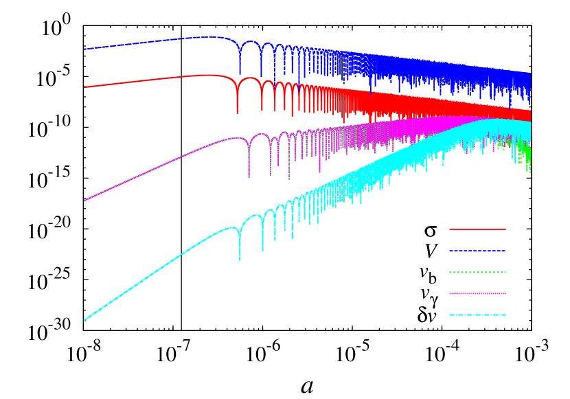
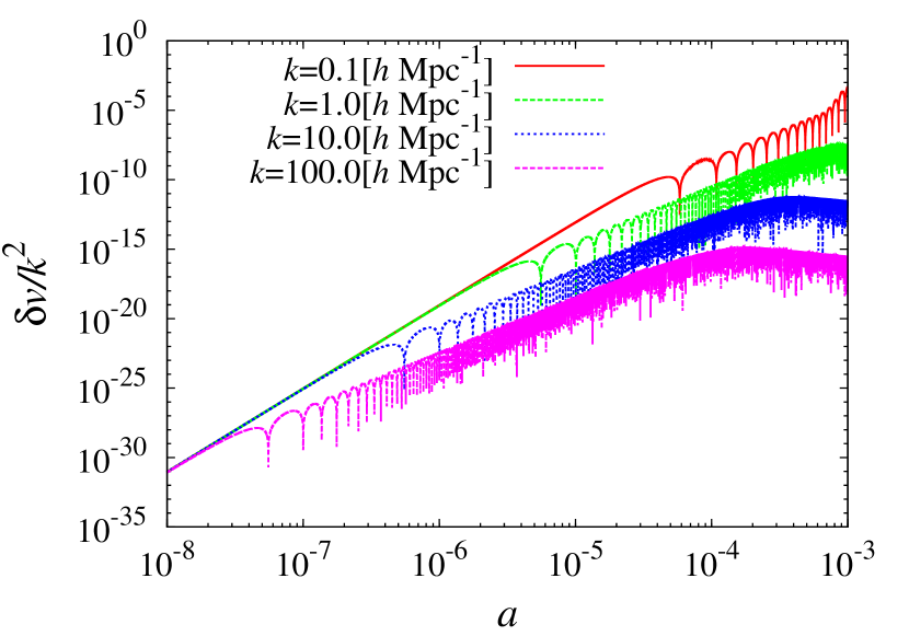
Figure 1: Time evolutions of perturbed variables in the Einstein-Aether gravity for the aether parameters fixed as Eq. (48) at $k=10\>h{\rm Mpc^{-1}}$. Shown in the left panel are the shear $\sigma$, the aether field $V$, the velocity of baryons $v_{b}$, the velocity of photons $v_{\gamma}$ and the velocity difference between baryons and photons $\delta v$. Black solid vertical line does not express a horizon entry time but “a sound horizon entry time”. The metric perturbation of the vector-mode $\sigma$ and the aether field start to decay not after the horizon crossing but after the sound horizon crossing. Subsequently, they start to oscillate and damp. In the right panel time evolutions of the velocity difference between baryons and photons $\delta v$ are shown for some wavenumbers as indicated. We normalized by the factor of $k^{2}$ to remove the scale dependence in early time (see the last paragraph of the previous section).

As mentioned earlier, the perturbation of the aether field $V$ and the metric perturbation $\sigma$ dominate over the other perturbation variables in the early universe. When the modes of $\delta v$ and $\sigma$ enter the sound horizon, they start to oscillate and decay in proportion to the inverse of the scale factor. On the contrary the baryon and the photon velocities increase until breaking the tight-coupling.

When the Fourier modes reach the Silk damping scale, perturbations in the photon fluid start to vanish exponentially along with the baryon velocity and the potential $\sigma$ in the absence of the aether field Ichiki et al. (2012). In contrast, in the presence of the aether field, such exponential damping does not appear as shown in Fig. 1. This is because the aether field can keep the vector potential $\sigma$ large enough, and push the photon fluid in equilibrium with $\sigma$ through the photon anisotropic stress even in the photon diffusion regime. The baryon velocity decays faster than the photon velocity in a particular case shown in Fig. 1 (green dashed line). This can be understood by noting the fact that baryons are non-relativistic having no anisotropic stress, and therefore their velocity is completely determined by the Compton drag force from the photon fluid independently of the metric perturbation $\sigma$ (see Eq. (38)). Because the photon velocity is sustained by the aether field and kept large enough even after the tight-coupling is broken down, the equation for the baryon velocity Eq. (38) is reduced to

$$\dot{v}_{b}\approx\frac{4\rho_{\gamma}}{3\rho_{b}}an_{e}\sigma_{T}v_{\gamma}\ .$$ (49)

Because the right hand side of the above equation starts to damp exponentially with rapid oscillations right before the recombination epoch, the baryon velocity also damps exponentially with oscillations. As a result, the difference of the velocities between baryons and photons has the same amplitude as the photon velocity at late time.

In Fig. 1, before crossing the sound horizon, the evolution of $\delta v$ may be explained by use of the tight-coupling approximations, i.e., Eqs. (22), (42) and (47). Since $\sigma$ and the aether field dominate the perturbation variables, we can ignore the photon velocity in Eq. (47). Then we have an approximate expression as

$$\delta v=-\frac{4}{15}\left(\frac{k}{\dot{\tau}}\right)^{2}\frac{R}{1+R}\sigma\ .$$ (50)

Substituting the time dependence of $\dot{\tau}$, $R$ and $\sigma$ during the radiation dominated era, the above equation is reduced to the simple form as $\delta v\propto k^{2}a^{5}\sigma\propto k^{2}a^{5+\nu_{\rm rad}}$. After crossing the sound horizon, $\delta v$ continues to grow until the tight-coupling is broken. Subsequently, the velocity difference between baryons and photons $\delta v$ decays together with $\sigma$ as discussed above.

To see the dependence of the aether parameters, we consider another parameter set:

$$\begin{split}c_{14}&=-0.9\times 10^{-10}\ ,\\ c_{13}&=-1.8\times 10^{-10}\ ,\\ \alpha=-c_{14}&=0.9\times 10^{-10}\ ,\\ c_{1}&=-0.9\times 10^{-10}\ ,\\ c^{2}_{v}&=1.0\ .\end{split}$$ (51)

The result is depicted in Fig. 1 and Fig. 2.

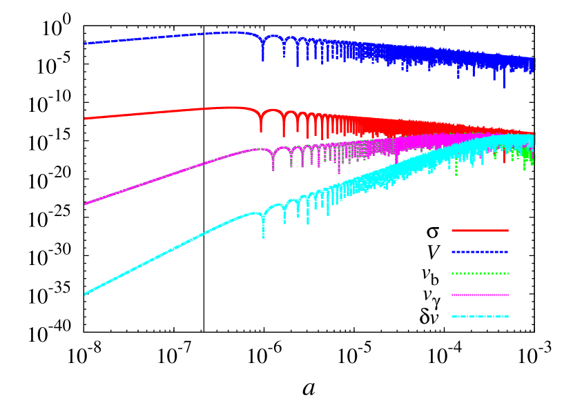
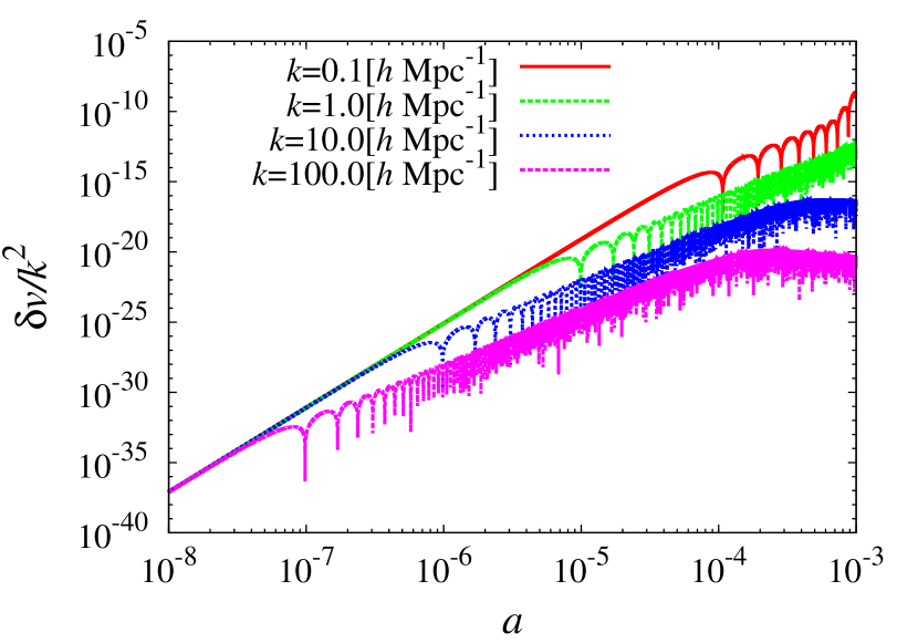
Figure 2: Same as Fig. 1 but for the different aether parameters fixed as Eq. (51).

The relation between $V$ and $\sigma$ obtained from Eq. (23) is indeed satisfied. We find that $\delta v$ in Fig. 2 is smaller than one in Fig. 1. If $c_{13}\ll 1$, we can rewrite the equation (23) as $\sigma\simeq-c_{13}V$. Because of this relation, $\sigma$ is suppressed by the factor of $c_{13}$ compared with $V$. Furthermore, we can see $\delta v\sim v_{\gamma}\sim\sigma$ at late time. Therefore, magnetic fields are also suppressed at late time by the factor of $c_{13}$ if $c_{13}\ll 1$.

IV.2 Power spectra of temperature and B-mode polarization

In this subsection, we calculate the power spectra of CMB temperature and B-mode polarization. We assume that the initial power spectrum of the aether field is given by a power law as Eq. (37). Although the initial amplitude $\mathcal{A}_{V}$ and spectral index $n_{v}$ may depend on the early universe model, following the discussion in Ref. Nakashima and Kobayashi (2011), we assume that

$$n_{v}=3-\sqrt{1-\frac{\alpha}{c_{14}}\frac{4\varepsilon}{(1-\varepsilon)^{2}}}\ ,$$ (52)

where $\varepsilon=1-\mathcal{H}^{\prime}/\mathcal{H}^{2}$ is the slow-roll parameter. In addition, we assume that the spectral index does not change in the scales of interest. The combination of the aether parameters $\alpha/c_{14}$ is constrained as $-1\leq\alpha/c_{14}\leq 0$ for perturbation of the aether field to have a growing mode solution in the radiation dominated era and the isocurvature mode does not grow, see Eq. (67). The spectral index is also constrained as $2-2\varepsilon/(1-\varepsilon)^{2}\lesssim n_{v}\leq 2$ for $\varepsilon\ll 1$, and thus we fix the spectral index as $n_{v}=2$ in our numerical calculations for simplicity. Since the aether amplitude may further change during the reheating stage, we treat the initial amplitude as a free parameter Nakashima and Kobayashi (2011).

Before moving to the calculation of the magnetic field spectrum, we can give a rough constraint on the initial amplitude and the aether parameters from the CMB temperature anisotropies. The CMB temperature (TT) and B-mode polarization (BB) power spectra for the fiducial parameter set are depicted in Fig. 3. From the figure we find that the TT power spectrum from the aether field looks similar to that from the primary tensor perturbations, with a slightly different horizon scale, i.e., the first peak location, as discussed in section IV. A. Therefore the constraint on the aether field from the TT power spectrum comes from the low multipole components, which is similar to the case of the primary tensor modes. As for the parameter dependence of the TT and BB power spectra, we find that the amplitudes of the spectra depend on the combination of the initial amplitude ${\cal A}_{V}$, the aether parameters $c_{13}$ and $c_{v}$ as ${\cal A}_{V}c_{13}^{2}c^{-4}_{v}$. One can understand this dependence as follows. First of all, the amplitude of the metric perturbation $\sigma$ is proportional to $c_{13}$ as shown in Eq. (23), and thus $C_{\ell}\propto\sigma^{2}\propto c_{13}^{2}$. Next, from Eqs. (26) and (28), the aether perturbation $V$ evolves as $V\propto\eta$ outside the sound horizon during the radiation dominated era while $V$ decays as $V\propto\eta^{-1}$ with oscillations inside the sound horizon. The resultant amplitude inside the sound horizon can be expressed as $V=V_{\rm ini}\left({\eta_{\ast}}/{\eta_{\rm ini}}\right)\left({\eta}/{\eta_{\ast}}\right)^{-1}$ where the subscript “ini” means the initial value and $\eta_{\ast}$ represents the epoch of sound horizon crossing, which is given by $\eta_{\ast}=c_{v}^{-1}$. Therefore $V\propto\eta_{\ast}^{2}=c_{v}^{-2}$ and the amplitude of the spectra will be changed in proportion to $c^{-4}_{v}$. Note that the peak positions of the spectra also depend on $c_{v}$. We show this dependence explicitly in Fig. 4.

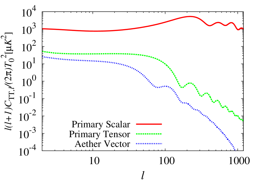
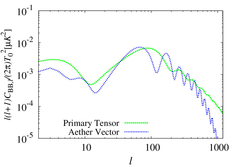
Figure 3: The CMB temperature and B-mode polarization anisotropy power spectra. “Primary Scalar” and “Primary Tensor” indicate the primary spectra from the scalar and tensor perturbations in the standard cosmology. “Aether Vector” indicates the spectra from the vector mode perturbation in the Einstein-Aether gravity. The aether parameters are set as $c_{14}=-1.0\times 10^{-4}$, $c_{13}=-2.0\times 10^{-4}$, $\alpha=1.0\times 10^{-4}$, $c_{1}=-3.0\times 10^{-2}$ and $c^{2}_{v}=3.0$. The initial amplitude and the spectral index are fixed as $\mathcal{A}_{V}c^{2}_{13}c^{-4}_{v}=2.0\times 10^{-17}$, and $n_{v}=2.0$ respectively. We assume that the tensor-to-scalar ratio is $r=0.1$.

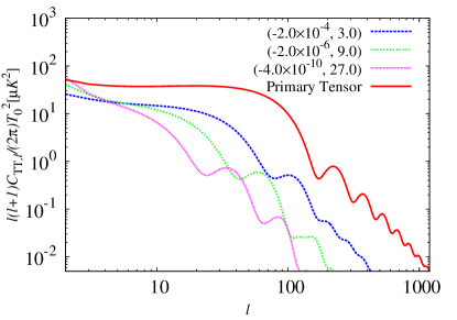
Figure 4: The CMB temperature anisotropy (TT) power spectra with different aether parameters; $c_{13}$ and $c_{v}$. Here we impose the condition, $\mathcal{A}_{V}c^{2}_{13}c^{-4}_{v}=2.0\times 10^{-17}$, on the aether parameters and the initial amplitude. “Primary Tensor” indicate the primary spectrum from the tensor perturbation in the standard cosmology. The spectra from the aether perturbation are depicted by solid lines, $(c_{13},\ c^{2}_{v})=$ $(-2.0\times 10^{-4},\ 3.0)$, $(-2.0\times 10^{-6},\ 9.0)$ and $(-4.0\times 10^{-10},\ 27.0)$, respectively. This figure suggests that if $\mathcal{A}_{V}c^{2}_{13}c^{-4}_{v}$ is fixed, the amplitudes of TT power spectra are almost the same at low multipoles. On the contrary, the peak locations are shifted. The TT power spectrum from tensor modes with $r=0.1$ is also plotted as a reference (broken line).

From the above discussion and Fig. 3, we find a new constraint on the aether parameters and the initial amplitude. Because the dependence of $C^{\rm aether}_{\ell}$ on the aether parameters is proportional to $\mathcal{A}_{V}c^{2}_{13}c^{-4}_{v}$, we find a relation from Fig. 3 as

$$C^{\rm aether}_{\ell\ TT}\approx C^{{\rm GW}(r=0.1)}_{\ell\ TT}\left(\frac{\mathcal{A}_{V}c^{2}_{13}c^{-4}_{v}}{2.0\times 10^{-17}}\right)\ ~{},$$ (53)

where $C^{{\rm GW}(r=0.1)}_{\ell\ TT}$ is the TT power spectrum by primordial gravitational waves with the scalar-tensor ratio $r=0.1$. By imposing $C^{\rm aether}_{\ell}\lesssim C^{{\rm GW}(r=0.1)}_{\ell\ TT}$, which is the current upper bound obtained by the WMAP team Bennett et al. (2012); Hinshaw et al. (2012), we can place a constraint on the aether parameters and the initial amplitude as

$$\mathcal{A}_{V}c^{2}_{13}c^{-4}_{v}\lesssim 2.0\times 10^{-17}\ .$$ (54)

When we assume the single field slow-roll inflation, the initial amplitude $\mathcal{A}_{V}$ is given in the aether parameters (See Appendix B). If we adopt Eq. (101), the above inequality can be rewritten as $c^{2}_{13}(-c_{14})^{-1}c^{-5}_{v}\lesssim 10^{43}$.

It should be noted that the B-mode power spectrum shows distinctive feature of oscillations at $\ell\gtrsim 80$, and thus future precise measurements of B-mode polarizations can be used to discriminate the contributions from the aether field and the primary tensor perturbations (Ref. Nakashima and Kobayashi (2011)). Note also that the aether field, with this upper bound on ${\cal A}_{V}c_{13}^{2}c^{-4}_{v}$, gives negligible contributions to the TE (E-mode and temperature cross correlation) and EE (E-mode auto correlation) power spectra compared to those from the standard (observed) density perturbations, and we have omitted them here.

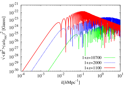
Figure 5: The spectrum of magnetic fields with $c_{14}=-1.0\times 10^{-4}$, $c_{13}=-2.0\times 10^{-4}$, $\alpha=1.0\times 10^{-4}$, $c_{1}=-3.0\times 10^{-4}$ and $c^{2}_{v}=3.0$ at $1+z=1100$, $1+z=2000$ and $1+z=10700$. The initial amplitude and the aether parameters are fixed as $\mathcal{A}_{V}c^{2}_{13}c^{-4}_{v}=2.0\times 10^{-17}$.

IV.3 Power spectrum of magnetic fields

The final results of generated magnetic fields spectra are depicted in Fig. 5. This figure shows that there are three characteristic scales. Let us focus on the scales, $10^{-4}\lesssim k/h{\rm Mpc^{-1}}\lesssim 10^{-2}$, which are outside the sound horizon at $1+z=2000$, right before the recombination epoch. In these scales, the magnetic field spectrum is proportional to $k^{4}$. Next, let us focus on the scales which are inside the sound horizon and in the tight-coupling regime ($\delta v\ll v_{\gamma}$) , $10^{-2}\lesssim k/h{\rm Mpc^{-1}}\lesssim 10^{0}$. In these scales the aether field begins to oscillate after the sound horizon entry. The velocity difference $\delta v$, the source of magnetic fields, also begins to oscillate because $\delta v$ is dragged by the aether field through $\sigma$ (see Eq. (50). The velocity difference grows with oscillations until the tight-coupling breaks down. In these scale, the spectrum of magnetic fields is proportional to $k^{1}$ with oscillations.

Finally we focus on the scales, $k/h{\rm Mpc^{-1}}\gtrsim 10^{0}$, in which the tight-coupling approximation is no longer valid. In these scales $\delta v\sim v_{\gamma}\sim\sigma$, and $\delta v$ begins to decay as $\propto a^{-1}$ together with $\sigma$. Consequently, the spectrum of magnetic fields decays with oscillations at $k/h{\rm Mpc^{-1}}\gtrsim 10^{0}$. As a result the spectrum of magnetic fields becomes proportional to $k^{-1}$ with oscillations.

At $1+z=1100$, the amplitude of magnetic fields has an extra enhancement due to the recombination process. When the Fourier mode is inside the sound horizon and in the tight-coupling regime, baryons oscillate with photons. The Fourier modes in this scale can have an extra growth because the tight-coupling becomes weaker as the recombination process takes place. On the other hand, there is little enhancement for the Fourier modes at scales where the tight-coupling has already been broken down at recombination. As a result, around the recombination epoch, the position of the peak of the spectrum moves slightly toward the smaller wavenumber.

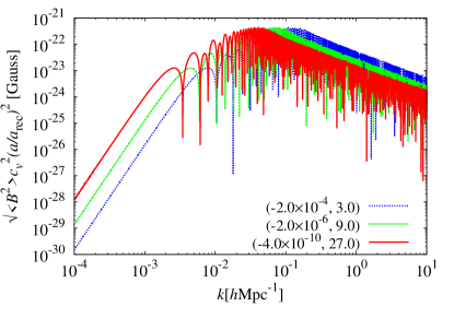
Figure 6: The spectrum of magnetic fields with difference of the aether parameters and the initial amplitude at $1+z=1100$. To normalize the amplitude of the spectra, we multiply by $c^{2}_{v}$. We impose only the condition, this condition is same as Fig. 4, $\mathcal{A}_{V}c^{2}_{13}c^{-4}_{v}=2.0\times 10^{-17}$, on the aether parameters and the initial amplitude. The spectra of the magnetic fields are depicted by solid lines, $(c_{13},\ c^{2}_{v})=$ $(-2.0\times 10^{-4},\ 3.0)$, $(-2.0\times 10^{-6},\ 9.0)$ and $(-4.0\times 10^{-10},\ 27.0)$, respectively.

Let us now estimate the largest amplitude of the magnetic fields allowed from the current observations. We find that the amplitude of the generated magnetic fields also depends on the combination of ${\cal A}_{V}c_{13}^{2}c^{-8}_{v}$. This aether parameter dependence can be understood in the same way as CMB power spectra as follows. Here we assume the universe is dominated by radiations. Magnetic fields are given as the time integral of the velocity difference $\delta v$ (Eq.(36)) as

$$\begin{split}\sqrt{a^{4}(t)\frac{k^{3}}{2\pi^{2}}S_{B}(k,t)}&=\left(\frac{4\sigma_{T}}{3e}\right)\sqrt{2\mathcal{P}_{V}(k)}k\int^{t}_{0}{dt^{\prime}a(t^{\prime})\rho_{\gamma}(t^{\prime})\delta v(k,t^{\prime})}\\ &\propto\int^{\eta}_{0}{d\eta^{\prime}\eta^{\prime 2}\rho_{\gamma}(\eta^{\prime})\delta v(k,\eta^{\prime})}\\ &\propto\int^{\eta}_{0}{d\eta^{\prime}\eta^{\prime-2}\delta v(k,\eta^{\prime})}\ .\end{split}$$ (55)

Time dependence of $\delta v$ has two characteristic epochs; the sound horizon crossing and the tight-coupling breakdown. Before the sound horizon crossing, $\delta v$ evolves as $\delta v\propto\eta^{6}$ as shown in Figs. 1 and 2, (also see Eq.  (50)). Once the Fourier mode enters the sound horizon, $\delta v$ evolves as $\delta v\propto\eta^{4}$ with oscillations. When the tight-coupling breaks down, moreover, $\delta v$ evolves as $\delta v\propto\eta^{-1}$ with oscillations. Therefore, by substituting the above time dependence into Eq. (55), we obtain the time dependence of magnetic fields as $B\propto\eta^{5}$, $\eta^{2}/c_{v}$, and $\eta^{-3}/c_{v}$, before and after sound horizon crossing, and after tight-coupling breakdown, respectively. Note that the above dependence of $\eta^{2}/c_{v}$ and $\eta^{-3}/c_{v}$ are obtained from the fact that $\int d\eta\eta^{n}e^{ikc_{v}\eta}\sim\eta^{n}/(ikc_{v})e^{ikc_{v}\eta}\sim\eta^{n}/c_{v}$. Accordingly, the dependence of magnetic fields on the aether parameters can be understood in the same way as CMB power spectra. $B\propto B_{\rm ini}(\eta_{\ast}/\eta_{\rm ini})^{5}\left((\eta_{\rm tc}/\eta_{*})^{2}/c_{v}\right)\left((\eta/\eta_{\rm tc})^{-3}/c_{v}\right)\propto c_{v}^{-5}c_{v}^{-1}c_{v}^{2}\propto c_{v}^{-4}$ where $\eta_{\ast}\propto c_{v}^{-1}$ and $\eta_{\rm tc}\propto c_{v}^{-1}$ are the epochs of sound horizon crossing and tight-coupling breakdown, respectively. Since the amplitude of $\delta v$ is proportional to $c_{13}$, the overall dependence is given by $B^{2}\propto{\cal A}_{V}c_{13}^{2}c^{-8}_{v}$, with ${\cal A}_{V}$ being the initial power spectrum amplitude. This dependence is explicitly depicted in Fig. 6. If $\mathcal{A}_{V}c^{2}_{13}c^{-8}_{v}$ is fixed, the amplitudes of generated magnetic fields are almost the same. Note that, however, peak positions of the magnetic field spectrum depend on $c_{v}$ as the CMB temperature anisotropy power spectrum.

Let us estimate the maximum amount of magnetic fields allowed from the limits of the CMB power spectra Eq. (54) and the constraint on the sound speed $c_{v}$ (Appendix A.5). We find that the spectrum of magnetic fields with aether field parameter dependence is given by

$$\sqrt{\Braket{B^{2}}}\sim\left\{\begin{array}[]{ll}\displaystyle 10^{-19}\left(\frac{\mathcal{A}_{V}c_{13}^{2}c^{-4}_{v}}{2.0\times 10^{-17}}\right)^{1/2}\left(\frac{c_{v}^{2}}{3}\right)^{-1}\left(\frac{k}{0.01\;h{\rm Mpc^{-1}}}\right)^{4}\;\left[{\rm Gauss}\right]&(k/h{\rm Mpc^{-1}}\lesssim 10^{-2}/c_{v})\\ \displaystyle 10^{-23}\left(\frac{\mathcal{A}_{V}c_{13}^{2}c^{-4}_{v}}{2.0\times 10^{-17}}\right)^{1/2}\left(\frac{c_{v}^{2}}{3}\right)^{-1}\left(\frac{k}{0.01\;h{\rm Mpc^{-1}}}\right)^{1}\;\left[{\rm Gauss}\right]&(10^{-2}/c_{v}\lesssim k/h{\rm Mpc^{-1}}\lesssim 1/c_{v})\\ \displaystyle 10^{-21}\left(\frac{\mathcal{A}_{V}c_{13}^{2}c^{-4}_{v}}{2.0\times 10^{-17}}\right)^{1/2}\left(\frac{c_{v}^{2}}{3}\right)^{-1}\left(\frac{k}{0.01\;h{\rm Mpc^{-1}}}\right)^{-1}\;\left[{\rm Gauss}\right]&(1/c_{v}\lesssim k/h{\rm Mpc^{-1}})\ .\\ \end{array}\right.$$ (59)

If we set ${\cal A}_{V}c_{13}^{2}c^{-4}_{v}=2.0\times 10^{-17}$ (Eq. (54)) and $c_{v}=1.0$, which satisfies the constraints in Appendix A, magnetic fields have the largest amplitude as $10^{-22}$ Gauss at $0.1\;h{\rm Mpc^{-1}}$.

V Summary

In this paper, we explored a mechanism of the generation of magnetic fields in the Einstein-Aether gravity. This theory contains a dynamical vector field, i.e., the aether field, and the aether field excites the metric perturbation of cosmological vector modes. Because the metric perturbation generates the velocity difference between baryons and photons, magnetic fields are naturally generated through Thomson scattering. This effect can arise only from the second order in the tight-coupling approximation. We derived solutions analytically up to the second order in the tight-coupling approximation to understand the results of the numerical calculations.

We investigated evolution of vector perturbations in detail in the Einstein Aether gravity. We found that the evolution of the vector metric perturbation $\sigma$ is quite different from the one with vector perturbations in General Relativity Ichiki et al. (2012). In particular, in the case with the aether field the Silk damping does not arise even after the tight coupling is broken down because $\sigma$ is large enough to support the velocity perturbation of photons. We checked that the Silk damping arises again if we turn off $\sigma$ by hand. We found that the amplitudes of CMB temperature and B-mode polarization power spectra depend on the initial amplitude and the aether parameters as $C_{\ell}\propto\mathcal{A}_{V}c^{2}_{13}c^{-4}_{v}$. By comparing the TT CMB power spectrum induced from the aether field with latest observations, we obtained a new constraint on the aether parameters as $\mathcal{A}_{V}c^{2}_{13}c^{-4}_{v}\lesssim 2.0\times 10^{-17}$.

In addition, we found the dependence of generated magnetic fields on the initial amplitude and the aether parameters as $\sqrt{\Braket{B^{2}}}\propto\mathcal{A}_{V}c^{2}_{13}c^{-8}_{v}$, which is slightly different from $C_{\ell}$’s. We then estimated the amplitude of magnetic fields with the aether parameters within the limits of current observations. We found that the maximum amount of magnetic fields can be as large as $\sqrt{\Braket{B^{2}}}\sim 10^{-22}$ Gauss at $k=0.1\;h{\rm Mpc^{-1}}$.

The shape of the magnetic field spectrum is also different from the one with vector perturbations in General Relativity Ichiki et al. (2012). First, the exponential cut-off in the magnetic field spectrum found in Ichiki et al. (2012) does not arise. The reason is exactly the same as in the case for the velocity perturbation of photons mentioned above since the source term, i.e., velocities, can survive the Silk damping effect. Second, since the vector-mode metric perturbation $\sigma$ decays inside the sound horizon, the velocity difference $\delta v$ also decays together with $\sigma$, once the tight-coupling between photons and baryons breaks down. Thus the spectrum of magnetic fields has a characteristic peak near the Silk damping scale at the recombination epoch. Moreover, around the recombination epoch, magnetic fields at larger scales than the peak scale experience a little enhancement due to the breakdown of the tight coupling, although the overall spectrum shape does not change very much.

It would be interesting to consider the generation of magnetic fields in other modified gravity theories or other inflation models which can amplify the initial power spectrum. For instance, the Einstein-Aether theory can be extended to have a more general kinetic term, so called $F(K)$ gravity Zuntz et al. (2010). It may also be interesting to constrain the aether parameters from other cosmological observations, for instance, the correlations or weak lensing effects of large scale structure. We leave these subjects for future works.

Appendix A Parameter constraints

In this appendix, we summarize the current observational and theoretical constraints on the aether parameters.

A.1 Effective gravitational constant

To have positive effective gravitational constants, $G_{\rm cos}$ and $G_{\rm N}$,

$$\alpha < 2$$ (60)

$$c_{14} > -2\ .$$ (61)

A.2 BBN constraint

The primordial helium abundance created by the Big-Bang Nucleosynthesis (BBN) is affected through the expansion rate of the universe via the Friedmann equation. Since the Friedmann equation (Eq. (16)) contains the aether parameters, the measurements of the primordial helium abundance can constrain the aether parameters as  Carroll and Lim (2004)

$$c_{14}+\alpha\lesssim 0.2\ .$$ (62)

This inequality can be easily satisfied if we set $c_{14}=-\alpha$. We assume this relation in our numerical calculations.

A.3 PPN limits

Parametrized post-Newtonian (PPN) parameters in the Einstein-Aether gravity have been derived and constrained in refs. Foster and Jacobson (2006); Eling and Jacobson (2004); Will (2006). PPN parameters in the Einstein-Aether gravity are reduced to two parameters $\alpha_{1}$ and $\alpha_{2}$ which are related to the aether parameters $c_{1},c_{2},c_{3}$ and $c_{4}$. The constraints from solar-system tests are written in the form as

$$\begin{split}\alpha_{1}&\equiv\frac{-8(c^{2}_{3}+c_{1}c_{4})}{2c_{1}-c^{2}_{1}+c^{2}_{3}}\lesssim 1.7\times 10^{-4}\ ,\\ \alpha_{2}&\equiv\frac{\alpha_{1}}{2}-\frac{(2c_{13}-c_{14})(\alpha+c_{14})}{c_{123}(2-c_{14})}\lesssim 1.2\times 10^{-7}\ .\end{split}$$ (63)

A.4 Stability of Scalar-Vector-Tensor perturbations

The linear perturbations in the Einstein-Aether gravity have been analyzed Armendariz-Picon et al. (2010). Scalar-, vector- and tensor-perturbations must be stable in the context of quantum and classical treatments. The classical stability imposes the condition that the square of the sound speed must be positive. The quantum stability imposes the condition that the ghost should not appear. In other words, the coefficient of a kinetic term of each mode must be positive. These conditions imply that

$$\begin{split}&1+c_{13}>0\ ,\\ &c_{14}\leq 0,\ c_{1}\leq\frac{c^{2}_{13}}{2(1+c_{13})}\ ,\\ &-2\leq c_{14}<0,\ c_{123}<0\ .\end{split}$$ (64)

A.5 Cherenkov radiation and Superluminal motion

If the sound speed of metric perturbations is smaller than the speed of light, the transverse-traceless graviton has sub-luminal dispersion Elliott et al. (2005). Accordingly, relativistic particles will lose its energy by emitting gravitons through a similar process of Cherenkov radiation. Therefore we can constrain the aether parameters from the fact that high energy cosmic rays have been observed on the Earth. However, we can avoid these constraints if we assume that all modes propagate super-luminally. The conditions of superluminal propagation are given in ref. Armendariz-Picon et al. (2010) as

$$\begin{split}(2+c_{14})c_{123}&\leq(2-\alpha)(1+c_{13})c_{14}\ ,\\ 2c_{4}&\geq\frac{-c^{2}_{13}}{1+c_{13}}\ ,\\ c_{13}&\leq 0\ .\end{split}$$ (65)

The connection of a superluminal propagation and a violation of causality is not trivial and has been still a matter of debate. In this paper, we assume that all modes propagate superluminally for simplicity.

A.6 Anisotropic stress

Anisotropic stress of long-wavelength adiabatic modes in scalar perturbations should not be too large Armendariz-Picon et al. (2010). From this we have a constraint as

$$|c_{13}|\lesssim 1\ .$$ (66)

A.7 Isocurvature mode

To prohibit isocurvature modes from being dominant at superhorizon scales, we find a constraint Armendariz-Picon et al. (2010):

$$\frac{\alpha}{c_{14}}\geq-1~{},$$ (67)

which is satisfied if we assume $c_{14}=-\alpha$.

A.8 Radiation damping

It is well known that the rate of orbital decay of the Hulse-Taylor binary B1913+16 matches the one induced by the emission of gravitational waves in General Relativity Stairs (2003); Will (2001). In the Einstein-Aether gravity, the deviation of the rate from General Relativity is controlled by the parameter ${\cal A}$

$$\mathcal{A}=\left(1+\frac{c_{14}}{2}\right)\left[\frac{1}{c_{t}}-\frac{2c_{14}c^{2}_{13}}{(2c_{1}+c^{2}_{1}-c^{2}_{3})^{2}}\frac{1}{c_{v}}-\frac{c_{14}}{6(2+c_{14})}\left(3+\frac{2\alpha_{2}-\alpha_{1}}{2(2c_{13}-c_{14})}\right)^{2}\frac{1}{c_{s}}\right]\ ,$$ (68)

where $\alpha_{1}$ and $\alpha_{2}$ are the PPN parameters, and $c_{s,v,t}$ are the sound speed of scalar-, vector- and tensor-perturbations Foster (2006). To match the observed rate, the parameter $\mathcal{A}$ is constrained as

$$|\mathcal{A}-1|\lesssim O(10^{-3})\ .$$ (69)

Appendix B Cosmological perturbations in Einstein-Aether gravity

Recently, perturbed Einstein-Aether gravity is discussed and formulated by Refs. Nakashima and Kobayashi (2011); Armendariz-Picon et al. (2010); Zuntz et al. (2010); Lim (2005); Zuntz et al. (2008). Here we summarize the cosmological perturbation theory in the Einstein-Aether gravity.

B.1 Perturbed equations

Here, we summarize the perturbed action and equations up to first order in real and Fourier spaces. In the synchronous gauge, the metric is given by

$$ds^{2}=a^{2}\left[-d\eta^{2}+\left(\delta_{ij}+h_{ij}\right)dx^{i}dx^{j}\right]\ .$$ (70)

The aether field is written as

$$\begin{split}A^{\mu}&=\left(\frac{1}{a},\frac{V^{i}}{a}\right)\ ,\\ A_{\mu}&=\left(-a,aV_{i}\right)\ .\end{split}$$ (71)

First, the equation of motion for the aether field, i.e., Eq. (6) leads to following equations. The $\mu=0$ component reads

$$-a^{2}\delta\lambda=(c_{2}+c_{3})\dot{V}^{k}_{\ ,k}-(2c_{1}+c_{2}+c_{3})\mathcal{H}V^{k}_{\ ,k}+c_{2}\frac{1}{2}\ddot{h}^{k}_{\ k}-(2c_{1}+c_{2}+2c_{3})\frac{1}{2}\mathcal{H}\dot{h}^{k}_{\ k}~{},$$ (72)

where $\delta\lambda$ is the variation of the Lagrange multiplier. We use Eq. (72) to remove $\delta\lambda$ from perturbed equations. The $\mu=i$ components are

$$\begin{split}c_{14}\left(\ddot{V}_{i}+2\mathcal{H}\dot{V}_{i}\right)&-(\alpha-c_{14})\mathcal{\dot{H}}V_{i}+(\alpha+c_{14})\mathcal{H}^{2}V_{i}\\ &-\left[c_{1}V_{i\ \ ,k}^{\ ,k}+(c_{2}+c_{3})V^{k}_{\ ,ik}+c_{2}\frac{1}{2}\dot{h}^{k}_{\ k,i}+(c_{1}+c_{3})\frac{1}{2}\dot{h}^{k}_{\ i,k}\right]=0\ .\end{split}$$ (73)

Second, we rewrite the Einstein equation (8) as

$$\begin{split}R_{\mu\nu}-\frac{1}{2}Rg_{\mu\nu}&=8\pi G\left(\frac{1}{8\pi G}T^{(A)}_{\mu\nu}+T^{(M)}_{\mu\nu}\right)\\ &\equiv 8\pi GT_{\mu\nu}\ .\end{split}$$ (74)

Then the perturbed Einstein equations lead to Shiraishi (2012):

$$\begin{split}&\ddot{h}^{i}_{\ i}+\mathcal{H}\dot{h}^{i}_{\ i}=8\pi Ga^{2}\left(\delta T^{0}_{\ 0}-\delta T^{i}_{\ i}\right)\ ,\\ &\ddot{h}^{i}_{\ j}+2\mathcal{H}\dot{h}^{i}_{\ j}+\mathcal{H}\dot{h}^{k}_{\ k}\delta^{i}_{\ j}-\left(\partial^{i}\partial_{j}h^{k}_{\ k}+\partial^{k}\partial_{k}h^{i}_{\ j}-\partial^{k}\partial_{j}h^{i}_{\ k}-\partial_{k}\partial^{i}h^{k}_{\ j}\right)=16\pi Ga^{2}\left(\delta T^{i}_{\ j}-\frac{1}{2}\delta^{i}_{\ j}\delta T^{\mu}_{\ \mu}\right)\ ,\\ &2\mathcal{H}\dot{h}^{i}_{\ i}+\partial^{j}\partial_{i}h^{i}_{\ j}-\partial^{k}\partial_{k}h^{i}_{\ i}=-16\pi Ga^{2}\delta T^{0}_{\ 0}\ ,\\ &\partial^{j}\dot{h}^{i}_{\ j}-\partial^{i}\dot{h}^{j}_{\ j}=16\pi Ga^{2}\delta T^{i}_{\ 0}\ .\end{split}$$ (75)

The perturbed energy momentum tensor for the aether field can be written in the form:

$$\begin{split}a^{2}\delta T^{(A)}{}^{0}_{\ 0}=&\left[c_{14}\dot{V}^{k}_{\ ,k}-(\alpha-c_{14})\mathcal{H}V^{k}_{\ ,k}-\alpha\frac{1}{2}\mathcal{H}\dot{h}^{k}_{\ k}\right]\ ,\\ a^{2}\delta T^{(A)}{}^{i}_{\ 0}=&-\left[c_{14}\ddot{V}^{i}+2c_{14}\mathcal{H}\dot{V}^{i}-(\alpha-c_{14})\mathcal{\dot{H}}V^{i}\right.\\ &\left.+(\alpha+c_{14})\mathcal{H}^{2}V^{i}+\frac{1}{2}(c_{1}-c_{3})\left(V^{k,i}_{\ \ \ ,k}-V_{\ \ \ ,k}^{i,k}\right)\right]\ ,\\ a^{2}\delta T^{(A)}{}^{i}_{\ j}=&-\left[c_{2}\left(\dot{V}^{k}_{\ ,k}+\frac{1}{2}\ddot{h}^{k}_{\ k}\right)+2c_{2}\left(\mathcal{H}V^{k}_{\ ,k}+\frac{1}{2}\mathcal{H}\dot{h}^{k}_{\ k}\right)\right]\delta^{i}_{\ j}\\ &-\left[\frac{1}{2}c_{13}\left(\dot{V}^{i}_{\ ,j}+\dot{V}^{\ ,i}_{j}+\ddot{h}^{i}_{\ j}\right)+c_{13}\mathcal{H}\left(V^{i}_{\ ,j}+V^{\ ,i}_{j}+\dot{h}^{i}_{\ j}\right)\right]\ .\end{split}$$ (76)

We obey the convention of the Fourier transformation as

$$f({\bf x},\eta)=\int{\frac{d^{3}{\bf k}}{(2\pi)^{3}}f({\bf k},\eta){\rm e}^{i{\bf k\cdot x}}}\ .$$ (77)

Furthermore we decompose these Fourier modes into scalar-, vector- and tensor-modes Shiraishi (2012). The definitions of the scalar, vector and tensor decompositions are

$$\begin{split}&\omega^{i}({\bf k},\eta)=\omega^{(0)}\mathcal{O}^{(0)i}+\sum_{\lambda=\pm 1}\omega^{(\lambda)}\mathcal{O}^{(\lambda)i}\ ,\\ &\chi_{ij}({\bf k},\eta)=-\frac{1}{3}\chi_{\rm iso}\delta_{ij}+\chi^{(0)}\mathcal{O}^{(0)}_{ij}+\sum_{\lambda=\pm 1}\chi^{(\lambda)}\mathcal{O}^{(\lambda)}_{ij}+\sum_{\lambda=\pm 2}\chi^{(\lambda)}\mathcal{O}^{(\lambda)}_{ij}\ .\end{split}$$ (78)

where $\mathcal{O}{{}^{(\lambda)}_{i}}$ and $\mathcal{O}^{(\lambda)}_{ij}$ are the projection operators for scalar ($\lambda=0$), vector ($\lambda=\pm 1$) and tensor ($\lambda=\pm 2$) modes. In the same way, the energy momentum tensor should be decomposed as

$$\begin{split}&\delta T^{i}_{\ 0}({\bf k},\eta)=\delta T^{(0)}_{v}\mathcal{O}^{(0)i}+\sum_{\lambda=\pm 1}\delta T^{(\lambda)}_{v}\mathcal{O}^{(\lambda)i}\ ,\\ &\delta T^{i}_{\ j}({\bf k},\eta)=-\frac{1}{3}\delta T^{\rm iso}_{t}\delta^{i}_{\ j}+\delta T^{(0)}_{t}\mathcal{O}^{(0)}{}^{i}_{\ j}+\sum_{\lambda=\pm 1}\delta T^{(\lambda)}_{t}\mathcal{O}^{(\lambda)}{}^{i}_{\ j}+\sum_{\lambda=\pm 2}\delta T^{(\lambda)}_{t}\mathcal{O}^{(\lambda)}{}^{i}_{\ j}\ .\end{split}$$ (79)

The perturbed energy momentum tensor for ordinary matter is expressed as

$$\begin{split}\delta T^{0}_{\ 0}&=-\rho\delta\ ,\\ \delta T^{\rm iso}_{t}&=-3p\Pi_{T}\ ,\\ \delta T^{(0)}_{v}&=-\left(\rho+p\right)v^{(s)}=-q^{(s)}\ ,\\ \delta T^{(0)}_{t}&=p\pi^{(s)}\ ,\\ \delta T^{(\pm 1)}_{v}&=-\left(\rho+p\right)v^{(v)}=-q^{(v)}\ ,\\ \delta T^{(\pm 1)}_{t}&=p\pi^{(v)}\ ,\\ \delta T^{(\pm 2)}_{t}&=p\pi^{(t)}\ .\end{split}$$ (80)

Then the Scalar-vector-tensor decomposition gives the following equations.

Scalar-mode

Equations of motion for the aether field are

$$\begin{split}&a^{2}\delta\lambda=(c_{2}+c_{3})k\dot{V}^{(0)}-(2c_{1}+c_{2}+c_{3})\mathcal{H}kV^{(0)}+\frac{1}{2}c_{2}\ddot{h}_{\rm iso}-\frac{1}{2}(2c_{1}+c_{2}+2c_{3})\mathcal{H}\dot{h}_{\rm iso}\ ,\\ &c_{14}\left(\ddot{V}^{(0)}+2\mathcal{H}\dot{V}^{(0)}\right)-(\alpha-c_{14})\mathcal{\dot{H}}V^{(0)}+(\alpha+c_{14})\mathcal{H}^{2}V^{(0)}+c_{123}k^{2}V^{(0)}+\frac{1}{3}c_{13}k\dot{h}^{(0)}+\frac{1}{6}\alpha k\dot{h}_{\rm iso}=0\ .\end{split}$$ (81)

The scalar components of the energy momentum tensor for the aether field are

$$\begin{split}a^{2}\delta T^{\rm iso}_{t}=&-\alpha\left[k\dot{V}^{(0)}+2\mathcal{H}kV^{(0)}+\frac{1}{2}\ddot{h}_{\rm iso}+\mathcal{H}\dot{h}_{\rm iso}\right]\ ,\\ a^{2}\delta T^{0}_{\ 0}=&-c_{14}k\dot{V}^{(0)}+(\alpha-c_{14})\mathcal{H}kV^{(0)}+\frac{1}{2}\alpha\mathcal{H}\dot{h}_{\rm iso}\ ,\\ a^{2}\delta T^{(0)}_{v}=&-c_{14}\left(\ddot{V}^{(0)}+2\mathcal{H}\dot{V}^{(0)}\right)+(\alpha-c_{14})\mathcal{\dot{H}}V^{(0)}-(\alpha+c_{14})\mathcal{H}^{2}V^{(0)}\ ,\\ a^{2}\delta T^{(0)}_{t}=&-\frac{1}{2}c_{13}\left(\ddot{h}^{(0)}+2\mathcal{H}\dot{h}^{(0)}\right)-c_{13}k\left(\dot{V}^{(0)}+2\mathcal{H}V^{(0)}\right)\ .\end{split}$$ (82)

The Einstein equations are

$$\begin{split}&\left(1-\frac{\alpha}{2}\right)\left(\ddot{h}_{\rm iso}+\mathcal{H}\dot{h}_{\rm iso}\right)=(\alpha+c_{14})\left(k\dot{V}^{(0)}+\mathcal{H}kV^{(0)}\right)+8\pi Ga^{2}\left(\rho\delta+3p\Pi_{T}\right)\ ,\\ &\left(1-\frac{\alpha}{2}\right)\mathcal{H}\dot{h}_{\rm iso}+\frac{k^{2}}{3}\left(h_{\rm iso}-h^{(0)}\right)=-c_{14}k\dot{V}^{(0)}+(\alpha-c_{14})\mathcal{H}kV^{(0)}-8\pi Ga^{2}\rho\delta\ ,\\ &k\left(\dot{h}_{\rm iso}-\dot{h}^{(0)}\right)=-3\left[c_{14}\left(\ddot{V}^{(0)}+2\mathcal{H}\dot{V}^{(0)}\right)-(\alpha-c_{14})\mathcal{\dot{H}}V^{(0)}+(\alpha+c_{14})\mathcal{H}^{2}V^{(0)}\right]-24\pi Ga^{2}q^{(s)}\ ,\\ &(1+c_{13})\left(\ddot{h}^{(0)}+2\mathcal{H}\dot{h}^{(0)}\right)+\frac{k^{2}}{3}\left(h_{\rm iso}-h^{(0)}\right)=-2c_{13}k\left(\dot{V}^{(0)}+2\mathcal{H}V^{(0)}\right)+16\pi Ga^{2}p\pi^{(s)}\ .\end{split}$$ (83)

Vector-mode

Equation of motion for the aether field is

$$c_{14}\left(\ddot{V}^{(\pm 1)}+2\mathcal{H}\dot{V}^{(\pm 1)}\right)-(\alpha-c_{14})\mathcal{\dot{H}}V^{(\pm 1)}+(\alpha+c_{14})\mathcal{H}^{2}V^{(\pm 1)}+c_{1}k^{2}V^{(\pm 1)}+\frac{1}{2}c_{13}k\dot{h}^{(\pm 1)}=0\ .$$ (84)

The vector components of the energy momentum tensor for the aether field are

$$\begin{split}a^{2}\delta T^{(\pm 1)}_{v}=&-c_{14}\left(\ddot{V}^{(\pm 1)}+2\mathcal{H}\dot{V}^{(\pm 1)}\right)+(\alpha-c_{14})\mathcal{\dot{H}}V^{(\pm 1)}-(\alpha+c_{14})\mathcal{H}^{2}V^{(\pm 1)}-\frac{1}{2}(c_{1}-c_{3})k^{2}V^{(\pm 1)}\\ =&\frac{1}{2}c_{13}k^{2}V^{(\pm 1)}+\frac{1}{2}c_{13}k\dot{h}^{(\pm 1)}\ ,\end{split}$$ (85)

and

$$a^{2}\delta T^{(\pm 1)}_{t}=-\frac{1}{2}c_{13}\left[k\dot{V}^{(\pm 1)}+2k\mathcal{H}V^{(\pm 1)}+\ddot{h}^{(\pm 1)}+2\mathcal{H}\dot{h}^{(\pm 1)}\right]\ ,$$ (86)

where we used Eq. (84) to derive the second line from the first line in Eq. (85). The Einstein equations are

$$\begin{split}\dot{\sigma}+2\mathcal{H}\sigma&=-\frac{c_{13}}{1+c_{13}}\left(\dot{V}+2\mathcal{H}V\right)-\frac{16\pi Ga^{2}p\pi^{(v)}}{(1+c_{13})k}\ ,\\ k^{2}\sigma&=\frac{1}{1+c_{13}}\left[16\pi Ga^{2}q-c_{13}k^{2}V\right]\ ,\end{split}$$ (87)

where we defined new variable $\sigma\equiv\dot{h}^{(\pm 1)}/k$.

Tensor-mode

The tensor component of the the energy momentum tensor for the aether field is

$$a^{2}\delta T^{(\pm 2)}_{t}=-\frac{1}{2}c_{13}\left(\ddot{h}^{(\pm 2)}+2\mathcal{H}\dot{h}^{(\pm 2)}\right)\ .$$ (88)

The Einstein equation is

$$\ddot{h}^{(\pm 2)}+2\mathcal{H}\dot{h}^{(\pm 2)}+\frac{k^{2}}{1+c_{13}}h^{(\pm 2)}=\frac{1}{1+c_{13}}16\pi Ga^{2}p\pi^{(t)}\ .$$ (89)

B.2 Perturbed action and initial power spectrum

In this subsection, we calculate perturbed action up to second order to obtain the initial power spectrum of the aether field at the end of inflation. For simplicity, the action is decomposed into each component as

$$S=S_{G}+S_{I}+S_{A}\ ,$$ (90)

where

$$\begin{split}&S_{G}=\frac{1}{16\pi G}\int{d^{4}x\sqrt{-g}R}\ ,\\ &S_{I}=\int{d^{4}x\sqrt{-g}\mathcal{L}_{I}}\ ,\\ &S_{A}=\frac{1}{16\pi G}\int{d^{4}x\sqrt{-g}\mathcal{L}_{A}}\ .\end{split}$$ (91)

Here $\mathcal{L}_{I}$ is the Lagrangian density for the inflaton field. Then the perturbed action up to second order is given by

$$\begin{split}S^{(2)}_{G}=\frac{1}{16\pi G}\int{d^{4}x}\frac{a^{2}}{4}&\left[\dot{h}^{k\ell}\dot{h}_{k\ell}-\dot{h}^{k}_{\ k}\dot{h}^{\ell}_{\ \ell}+\left(4\mathcal{H}^{2}+5\mathcal{\dot{H}}\right)h^{k}_{\ k}h^{\ell}_{\ \ell}+\left(-2\mathcal{H}^{2}-4\mathcal{\dot{H}}\right)h^{k\ell}h_{k\ell}\right.\\ &\left.h^{k}_{\ k,j}h^{\ell\ ,j}_{\ \ell}-h^{k\ell}_{\ \ ,j}h^{\ \ ,j}_{k\ell}-2h^{k}_{\ k,\ell}h^{\ell j}_{\ \ ,j}+2h^{k}_{\ j,k}h^{\ell j}_{\ \ ,\ell}\right]\ ,\end{split}$$ (92)

$$S^{(2)}_{I}=\frac{1}{16\pi G}\int{d^{4}x}\frac{a^{2}}{4}\left[\left(2\mathcal{H}^{2}+4\mathcal{\dot{H}}\right)\left(h^{k\ell}h_{k\ell}-h^{k}_{\ k}h^{\ell}_{\ \ell}\right)-\alpha\left(\mathcal{H}^{2}+2\mathcal{\dot{H}}\right)\left(h^{k\ell}h_{k\ell}-h^{k}_{\ k}h^{\ell}_{\ \ell}\right)\right]\ ,$$ (93)

$$\begin{split}S^{(2)}_{A}=\frac{1}{16\pi G}\int{d^{4}xa^{2}}&\left[-c_{14}\dot{V}^{i}\dot{V}_{i}+(\alpha+c_{14})\mathcal{H}^{2}V^{i}V_{i}-(\alpha-c_{14})\dot{\mathcal{H}}V^{i}V_{i}\right.\\ &+\frac{1}{4}\alpha\left(\mathcal{H}^{2}+2\mathcal{\dot{H}}\right)h^{k\ell}h_{k\ell}+\frac{1}{4}\alpha\left(\mathcal{H}^{2}-\mathcal{\dot{H}}\right)h^{k}_{\ k}h^{\ell}_{\ \ell}\\ &+c_{1}\left(V_{\ell}^{\ ,k}+\frac{1}{2}\dot{h}_{\ell}^{\ k}\right)\left(V^{\ell}_{\ ,k}+\frac{1}{2}\dot{h}^{\ell}_{\ k}\right)+c_{2}\left(V^{\ell}_{\ ,\ell}+\frac{1}{2}\dot{h}^{\ell}_{\ \ell}\right)\left(V^{k}_{\ ,k}+\frac{1}{2}\dot{h}^{k}_{\ k}\right)\\ &\left.+c_{3}\left(V^{k}_{\ ,\ell}+\frac{1}{2}\dot{h}^{k}_{\ \ell}\right)\left(V^{\ell}_{\ ,k}+\frac{1}{2}\dot{h}^{\ell}_{\ k}\right)\right]\ .\end{split}$$ (94)

Here, we employed the single field slow-roll inflation model and replaced the inflaton field with ${\cal H}$ and metric perturbations by using the Einstein equations and the equation of motion for the inflaton.

Hereafter we focus on the vector-mode only. By performing Fourier transformation and scalar-vector-tensor decomposition, we have

$$S^{(2)}_{\rm vec}=\frac{1}{2}\int{d\eta}\int{\frac{d^{3}{\bf k}}{(2\pi)^{3}}}\left[\left|\dot{v}\right|^{2}-\frac{\alpha}{c_{14}}\varepsilon\mathcal{H}^{2}\left|v\right|^{2}-c^{2}_{v}k^{2}\left|v\right|^{2}\right]\ ,$$ (95)

where $v\equiv\sqrt{-c_{14}}aV/\sqrt{8\pi G}$ and $\mathcal{H}^{2}-\mathcal{\dot{H}}=\varepsilon\mathcal{H}^{2}$. Through variation with respect to $v$, we have the equation of motion for the vector perturbation as

$$\ddot{v}_{k}+c^{2}_{v}k^{2}v_{k}+\frac{\alpha}{c_{14}}\varepsilon\mathcal{H}^{2}v_{k}=0\ .$$ (96)

Supposing that the slow-roll parameter $\varepsilon$ is constant during inflation, the conformal time $\eta$ and the scale factor $a$ are expressed as

$$\eta=-\frac{1}{\mathcal{H}}\frac{1}{1-\varepsilon},\ \ \frac{a}{a_{I}}=\left(\frac{\eta}{\eta_{I}}\right)^{1/(\varepsilon-1)}\ ,$$ (97)

where $\eta_{\rm I}$ and $a_{\rm I}$ are the conformal time and scale factor at the end of inflation. Then we can solve Eq. (96) easily to obtain

$$v_{k}(\eta)=\sqrt{\frac{\pi}{4}}(-\eta)^{1/2}{\rm e}^{i(2\nu_{\rm inf}+1)\pi/4}H^{(1)}_{\nu_{\rm inf}}(-kc_{v}\eta)\ ,$$ (98)

where $\nu_{\rm inf}=\sqrt{\frac{1}{4}-\frac{\alpha}{c_{14}}\frac{\varepsilon}{(1-\varepsilon)^{2}}}$ and $H^{(1)}_{\nu}$ is the Hankel function of the first kind. Finally the power spectrum of the aether field at the end of inflation is given by

$$\Braket{V(\eta,{\bf k})V^{*}(\eta,{\bf k^{\prime}})}=(2\pi)^{3}\frac{2\pi^{2}}{k^{3}}\mathcal{P}_{V}(k)\delta({\bf k}-{\bf k^{\prime}})\ ,$$ (99)

where

$$\begin{split}&\mathcal{P}_{V}(k,\eta_{\rm I})=\frac{(1-\varepsilon)^{2}}{-c_{14}}\frac{H_{\rm I}^{2}}{(8\pi G)^{-1}}\Gamma^{2}(\nu_{\rm inf})\left(\frac{c_{v}}{2}\right)^{-2\nu_{\rm inf}}\left(-k_{0}\eta_{\rm I}\right)^{n_{v}}\left(\frac{k}{k_{0}}\right)^{n_{v}}\ ,\end{split}$$ (100)

with $k_{0}=0.002{\rm Mpc^{-1}}$ and $n_{v}=3-2\nu_{\rm inf}$. From the above equation, we can read off the amplitude of the initial power spectrum as

$$\mathcal{A}_{V}=\frac{(1-\varepsilon)^{2}}{-c_{14}}\frac{H_{\rm I}^{2}}{(8\pi G)^{-1}}\Gamma^{2}(\nu_{\rm inf})\left(\frac{c_{v}}{2}\right)^{-2\nu_{\rm inf}}\left(-k_{0}\eta_{\rm I}\right)^{n_{v}}\ .$$ (101)

If we substitute the above amplitude into Eq. (54) with the condition that $c_{14}=-\alpha$, the inequality Eq. (54) can be rewritten as

$$\frac{c^{2}_{13}}{(-c_{14}c^{5}_{v})}\lesssim 10^{43}\ ,$$ (102)

where we have assumed $\varepsilon\simeq 0.16$, which corresponds to the scalar-tensor ratio $r\simeq 0.1$, $H_{\rm I}\simeq 5\times 10^{13}$ GeV, and $\eta_{\rm I}\simeq-2.0\times 10^{15}$ GeV.

References

- Giovannini (2004) M. Giovannini, Int.J.Mod.Phys. D13, 391 (2004), eprint astro-ph/0312614.
- Widrow (2002) L. M. Widrow, Rev.Mod.Phys. 74, 775 (2002), eprint astro-ph/0207240.
- Ryu et al. (2012) D. Ryu, D. R. Schleicher, R. A. Treumann, C. G. Tsagas, and L. M. Widrow, Space Sci.Rev. 166, 1 (2012), eprint 1109.4055.
- Neronov and Vovk (2010) A. Neronov and I. Vovk, Science 328, 73 (2010), eprint 1006.3504.
- Pandey and Sethi (2013) K. L. Pandey and S. K. Sethi, The Astrophysical Journal 762, 15 (2013).
- Widrow et al. (2012) L. M. Widrow, D. Ryu, D. R. Schleicher, K. Subramanian, C. G. Tsagas, et al., Space Sci.Rev. 166, 37 (2012), eprint 1109.4052.
- Davis et al. (1999) A.-C. Davis, M. Lilley, and O. Tornkvist, Phys.Rev. D60, 021301 (1999), eprint astro-ph/9904022.
- Martin and Yokoyama (2008) J. Martin and J. Yokoyama, JCAP 0801, 025 (2008), eprint 0711.4307.
- Subramanian (2010) K. Subramanian, Astron.Nachr. 331, 110 (2010), eprint 0911.4771.
- Demozzi et al. (2009) V. Demozzi, V. Mukhanov, and H. Rubinstein, JCAP 0908, 025 (2009), eprint 0907.1030.
- Kanno et al. (2009) S. Kanno, J. Soda, and M.-a. Watanabe, JCAP 0912, 009 (2009), eprint 0908.3509.
- Fujita and Mukohyama (2012) T. Fujita and S. Mukohyama, JCAP 1210, 034 (2012), eprint 1205.5031.
- Paoletti and Finelli (2012) D. Paoletti and F. Finelli (2012), eprint 1208.2625.
- Yamazaki et al. (2012) D. G. Yamazaki, T. Kajino, G. J. Mathew, and K. Ichiki, Phys.Rept. 517, 141 (2012), eprint 1204.3669.
- Fedeli and Moscardini (2012) C. Fedeli and L. Moscardini (2012), eprint 1209.6332.
- Biermann and Schlüter (1951) L. Biermann and A. Schlüter, Physical Review 82, 863 (1951).
- Kemp (1982) J. C. Kemp, PASP 94, 627 (1982).
- Hanayama et al. (2005) H. Hanayama, K. Takahashi, K. Kotake, M. Oguri, K. Ichiki, et al., Astrophys.J. 633, 941 (2005), eprint astro-ph/0501538.
- Miranda et al. (1998) O. D. Miranda, M. Opher, and R. Opher, Mon.Not.Roy.Astron.Soc. (1998), eprint astro-ph/9808161.
- Kulsrud et al. (1997) R. M. Kulsrud, R. Cen, J. P. Ostriker, and D. Ryu, Astrophys.J. 480, 481 (1997), eprint astro-ph/9607141.
- Gnedin et al. (2000) N. Y. Gnedin, A. Ferrara, and E. G. Zweibel, Astrophys.J. 539, 505 (2000), eprint astro-ph/0001066.
- Takahashi et al. (in preparation.) K. Takahashi, M. Mori, K. Ichiki, and S. Inoue (in preparation.).
- Harrison (1970) E. R. Harrison, Mon. Not. Roy. Astron. Soc. 147, 279 (1970).
- Lewis (2004) A. Lewis, Phys.Rev. D70, 043518 (2004), eprint astro-ph/0403583.
- Ichiki et al. (2012) K. Ichiki, K. Takahashi, and N. Sugiyama, Phys.Rev. D85, 043009 (2012), eprint 1112.4705.
- Hollenstein et al. (2008) L. Hollenstein, C. Caprini, R. Crittenden, and R. Maartens, Phys.Rev. D77, 063517 (2008), eprint 0712.1667.
- Takahashi et al. (2005) K. Takahashi, K. Ichiki, H. Ohno, and H. Hanayama, Phys.Rev.Lett. 95, 121301 (2005), eprint astro-ph/0502283.
- Fenu et al. (2011) E. Fenu, C. Pitrou, and R. Maartens, Mon.Not.Roy.Astron.Soc. 414, 2354 (2011), eprint 1012.2958.
- Jacobson and Mattingly (2001) T. Jacobson and D. Mattingly, Phys.Rev. D64, 024028 (2001), eprint gr-qc/0007031.
- Jacobson (2010) T. Jacobson, Phys.Rev. D81, 101502 (2010), eprint 1001.4823.
- Blas et al. (2010) D. Blas, O. Pujolas, and S. Sibiryakov, Phys.Rev.Lett. 104, 181302 (2010), eprint 0909.3525.
- Horava (2009a) P. Horava, Phys.Rev. D79, 084008 (2009a), eprint 0901.3775.
- Horava (2009b) P. Horava, JHEP 0903, 020 (2009b), eprint 0812.4287.
- Zlosnik et al. (2008) T. G. Zlosnik, P. G. Ferreira, and G. D. Starkman, Phys. Rev. D 77, 084010 (2008), URL http://link.aps.org/doi/10.1103/PhysRevD.77.084010.
- Zuntz et al. (2010) J. Zuntz, T. Zlosnik, F. Bourliot, P. Ferreira, and G. Starkman, Phys.Rev. D81, 104015 (2010), eprint 1002.0849.
- Meng and Du (2012) X. Meng and X. Du, Physics Letters B 710, 493 (2012).
- Barrow (2012) J. D. Barrow, Phys.Rev. D85, 047503 (2012), eprint 1201.2882.
- Lim (2005) E. A. Lim, Phys.Rev. D71, 063504 (2005), eprint astro-ph/0407437.
- Zuntz et al. (2008) J. A. Zuntz, P. Ferreira, and T. Zlosnik, Phys.Rev.Lett. 101, 261102 (2008), eprint 0808.1824.
- Eling et al. (2007) C. Eling, T. Jacobson, and M. Coleman Miller, Phys.Rev. D76, 042003 (2007), eprint 0705.1565.
- Garfinkle et al. (2007) D. Garfinkle, C. Eling, and T. Jacobson, Phys.Rev. D76, 024003 (2007), eprint gr-qc/0703093.
- Eling and Jacobson (2006) C. Eling and T. Jacobson, Class.Quant.Grav. 23, 5643 (2006), eprint gr-qc/0604088.
- Armendariz-Picon and Diez-Tejedor (2009) C. Armendariz-Picon and A. Diez-Tejedor, JCAP 0912, 018 (2009), eprint 0904.0809.
- Armendariz-Picon et al. (2010) C. Armendariz-Picon, N. F. Sierra, and J. Garriga, JCAP 1007, 010 (2010), eprint 1003.1283.
- Carroll and Lim (2004) S. M. Carroll and E. A. Lim, Phys.Rev. D70, 123525 (2004), eprint hep-th/0407149.
- Ichiki et al. (2006) K. Ichiki, K. Takahashi, H. Ohno, H. Hanayama, and N. Sugiyama, Science 311, 827 (2006), eprint arXiv:astro-ph/0603631.
- Maeda et al. (2009) S. Maeda, S. Kitagawa, T. Kobayashi, and T. Shiromizu, Classical and Quantum Gravity 26, 135014 (2009), eprint 0805.0169.
- Nakashima and Kobayashi (2011) M. Nakashima and T. Kobayashi, Phys.Rev. D84, 084051 (2011), eprint 1103.2197.
- Lewis et al. (2000) A. Lewis, A. Challinor, and A. Lasenby, Astrophys.J. 538, 473 (2000), eprint astro-ph/9911177.
- Bennett et al. (2012) C. Bennett, D. Larson, J. Weiland, N. Jarosik, G. Hinshaw, et al. (2012), eprint 1212.5225.
- Hinshaw et al. (2012) G. Hinshaw, D. Larson, E. Komatsu, D. Spergel, C. Bennett, et al. (2012), eprint 1212.5226.
- Foster and Jacobson (2006) B. Z. Foster and T. Jacobson, Phys.Rev. D73, 064015 (2006), eprint gr-qc/0509083.
- Eling and Jacobson (2004) C. Eling and T. Jacobson, Phys.Rev. D69, 064005 (2004), eprint gr-qc/0310044.
- Will (2006) C. M. Will, Living Rev.Rel. 9, 3 (2006), eprint gr-qc/0510072.
- Elliott et al. (2005) J. W. Elliott, G. D. Moore, and H. Stoica, JHEP 0508, 066 (2005), eprint hep-ph/0505211.
- Stairs (2003) I. H. Stairs, Living Rev.Rel. 6, 5 (2003), eprint astro-ph/0307536.
- Will (2001) C. M. Will, Living Rev.Rel. 4, 4 (2001), eprint gr-qc/0103036.
- Foster (2006) B. Z. Foster, Phys.Rev. D73, 104012 (2006), eprint gr-qc/0602004.
- Shiraishi (2012) M. Shiraishi (2012), eprint 1210.2518.