A Class of Solvable Optimal Stopping Problems of Spectrally Negative Jump Diffusions

Abstract

We consider the optimal stopping of a class of spectrally negative jump diffusions. We state a set of conditions under which the value is shown to have a representation in terms of an ordinary nonlinear programming problem. We establish a connection between the considered problem and a stopping problem of an associated continuous diffusion process and demonstrate how this connection may be applied for characterizing the stopping policy and its value. We also establish a set of typically satisfied conditions under which increased volatility as well as higher jump-intensity decelerates rational exercise by increasing the value and expanding the continuation region.

Keywords: jump diffusions, optimal stopping, nonlinear programming, certainty equivalence

AMS subject classification: 60G40, 60J60, 60J75

1 Introduction

It is a well-known result from literature on mathematical finance that the price of a perpetual American option on an underlying asset whose value can be characterized as a stochastic process coincides with the value of an optimal stopping problem for this process (see, for example, Karatzas and Shreve, (1999) pp. 54–87 and Øksendal, (2003), pp. 290–298). Such option prices, while naturally of interest in themselves, can also be used as upper bounds for prices of American options with finite expiration dates. Thus, their role is of importance from a risk management point of view as well. Perpetual optimal stopping problems arise quite naturally also in the real options literature on the valuation of irreversible investment opportunities (see Dixit and Pindyck, (1994) for an extensive textbook treatment of this theory, and Boyarchenko and Levendorskiĭ, (2007) for some more recent developments in this field). In that modeling framework the investment decision is usually interpreted as an opportunity but not an obligation to obtain a stochastically fluctuating return in exchange from a payment (sunk cost) which may or may not be stochastic as well. Given the considerable planning horizon of the valuation of real investment opportunities, the time horizon is typically assumed to be infinite, i.e. the considered optimal timing problem of the investment opportunity is assumed to be perpetual.

When the dynamics of the underlying process are characterizable via an Itô stochastic differential equation of form

$$dX_{t}=\alpha(X_{t})dt+\sigma(X_{t})dW_{t}$$ (1)

with $W$ a standard Wiener process, the stopping problem has been widely studied by relying on various techniques. Perhaps the most common approach is to rely on variational inequalities or the classical Hamilton-Jacobi-Bellman approach due to its applicability in a multidimensional setting as well (cf. Øksendal, (2003) and Øksendal and Reikvam, (1998)). In the one-dimensional setting there are, however, several different techniques for analyzing the perpetual stopping problem. The most general approach is probably provided by studies relying on the integral characterization of excessive functions for diffusion processes and the Martin boundary theory (cf. Salminen, (1985) and Borodin and Salminen, (2002), pp. 32–35). Alternatively, the considered problem can be analyzed by relying on techniques based on martingales like the Snell envelope (see Peskir and Shiryaev, (2006) for a thorough characterization and comprehensive list of references), or the Beibel-Lerche approach (see, for example, Beibel and Lerche, (1997) and Lerche and Urusov, (2007)). One dimensional stopping problems have been also analyzed by exploiting the relationship between functional concavity and $r$-excessivity along the lines of the pioneering work by Dynkin, (1965) (Chapters XV and XVI) and by Dynkin and Yuskevich, (1969) which has been subsequently applied within a general optimal stopping framework in Dayanik and Karatzas, (2003). An approach based on occupation measures and infinite dimensional linear programming is, in turn, developed in Cho and Stockbridge, (2002) and Helmes and Stockbridge, (2007). Another technique for studying the perpetual optimal stopping problem in the linear diffusion setting is provided by the approaches relying on the well-known relationship between excessivity and superharmonicity with respect to first exit times from open sets with compact closure in the state space of the considered diffusion (cf. Dynkin, (1965), Theorem 12.4). In this case, the optimal stopping problem is reduced to the optimization of arbitrary boundaries and can be analyzed by relying on ordinary nonlinear programming techniques (cf. Alvarez, (2001) and Alvarez, (2004)).

More recently, the shortcomings of continuous path models driven by a Brownian motion have become apparent and, consequently, more general models allowing path discontinuities have been studied. In many ways the most simple generalizations of the traditional continuous path models are jump diffusion models, in which the driving noise is a Lévy process. Lévy processes can be used to construct more realistic models of financial quantities, as they are able to generate jump discontinuities and the leptokurtic feature of return distributions, unlike the Gaussian models based on a Brownian motion and the normal distribution. For a taste of the plentiful research done on pricing American options and optimal stopping in Lévy models, see (for example) Alili and Kyprianou, (2005), Boyarchenko and Levendorskiĭ, (2002), Boyarchenko and Levendorskiĭ, (2005), Duffie et al, (2000), Gerber and Landry, (1998), Gerber and Shiu, (1998), Kou, (2002), Mordecki, 2002a , Mordecki, 2002b Mordecki and Salminen, (2007), and Pham, (1997).

In risk management a criticism often leveled against the continuous models is their inability to model downside risk: the possibility of an instantaneous drop in the value of an asset. In real life markets phenomena closely resembling such instantaneous drops are often observed (for example, sudden unanticipated deterioration of stock market values, credit defaults, etc.). An empirically observed fact is that in the stock market reactions to negative shocks are usually significantly stronger than the reactions to positive ones (this is the celebrated ”bad news” principle originally introduced in the seminal study by Bernanke, (1983)). In light of this asymmetric nature of the reaction to unanticipated shocks, a prudent approach is to disregard possibilities for positive surprises and to take fully into account the possibilities for disadvantageous future occurrences. Consequently, a one-sided model that allows instantaneous downward jumps can be seen as an acceptable model from a prudent risk management point of view.

Motivated by our previous arguments, it is our objective in this study to consider a spectrally negative one-dimensional jump diffusion, say $X$, with a state space $\mathcal{I}=(a,b)\subseteq\mathbb{R}$ and unattainable boundaries $a$ and $b$. Interestingly, we establish that given some extra conditions on $X$, the value of the optimal stopping problem has a representation in terms of an ordinary nonlinear programming problem (cf. Alvarez, (2001) and Alvarez, (2003) for an associated result in the continuous diffusion case).

In order to develop relatively easily verifiable sufficient conditions we consider an optimal stopping problem of an associated continuous diffusion process which can be obtained by removing the pure jump part of the considered Lévy diffusion. We demonstrate that the value of the considered jump-diffusion stopping problem can be ”sandwiched” between the values of two stopping problems which are defined with respect to the associated continuous diffusion. This finding is of interest since it can be applied for deriving bounds for the exercise threshold of the considered optimal stopping problem for the underlying jump-diffusion. Moreover, since the restricting values defined with respect to the continuous diffusion differ only by the rate at which they are discounted, our findings indicate that under some circumstances the downside jump-risk can be directly incorporated into the continuous diffusion case by adjusting the discount rate appropriately (for some results in this direction, see Alvarez and Rakkolainen, (2010)). This characterization is also important in the analysis of the impact of downside risk on the optimal stopping policy since according to this representation the optimal exercise boundary is lower for the underlying jump-diffusion than for the associated dominating continuous diffusion process provided that both valuations are discounted at the same rate.

We also investigate the comparative static properties of the optimal stopping policy and its value and present a set of relatively general conditions under which the value of the considered problem is convex. Along the lines of previous studies considering the optimal stopping of linear diffusions, we find that in such a case higher volatility increases the value of the optimal strategy and expands the continuation region where stopping is suboptimal by increasing the optimal exercise threshold. These observations are of interest since they indicate that higher volatility decelerates the rational exercise of investment opportunities by increasing the option value of waiting in the presence of jumps as well. Interestingly, our results also indicate that higher jump-intensity increases the value of waiting and decelerates rational exercise by expanding the continuation region. These observations emphasize the potentially significant combined negative effect of jump-risk and continuous systematic risk on the timing of irreversible investment policies.

We also analyze if the considered class of stopping problems can be expressed in terms of an associated deterministic timing problem. Somewhat surprisingly, we find that the value of the considered optimal stopping problem coincides with the value of an associated optimal timing problem of a deterministic process evolving according to the dynamics characterized by an ordinary first order differential equation adjusted to the risk generated by the driving Lévy process. We show that this representation is valid for single threshold policies within the considered class of stopping problems. Since an analogous certainty equivalent formulation is valid in the continuous diffusion setting as well, our findings can be utilized in decomposing the required exercise premium into two parts: a part based on the continuous Brownian dynamics and a part based on the discontinuous compensated compound Poisson process.

The contents of this study are as follows. In section 2, we present the model and the basic assumptions used throughout the study. The auxiliary results based on the associated continuous diffusion are then developed in section 3. The representation of the stopping problem in terms of an ordinary optimization problem is then stated and proved in section 4. The sensitivity of the optimal exercise policy and its value with respect to changes in volatility and the jump intensity of the driving dynamics are then investigated in section 5. Section 6 in turn summarizes our results on the certainty equivalent valuation principles. Explicit illustrations are given in section 7, and section 8 finally concludes our study.

2 The Setup and Basic Assumptions

Let $(\Omega,\mathcal{F},\mathbb{P})$ be a probability space carrying a standard Wiener process $W=\{W_{t}\}$ and a compound Poisson process $J=\{J_{t}\}$ with intensity $\lambda$ and a jump size distribution on $\mathcal{S}\subseteq\mathbb{R}$ characterized by a probability distribution $\mathfrak{m}$. We define a Lévy process $L=\{L_{t}\}$ by

$$L_{t}=t+W_{t}+J_{t}.$$ (2)

We equip $(\Omega,\mathcal{F},\mathbb{P})$ with the completed natural filtration $\mathbb{F}$ generated by this process. The natural filtration of a Lévy process is right-continuous, and thus the completed filtration satisfies the usual hypotheses (see Protter, (2004) Theorem I.31).

Given the driving Lévy process, let $X=\{X_{t}\}$ be a jump diffusion evolving according to the dynamics characterized by the stochastic differential equation

$$dX_{t}=\alpha(X_{t-})dt+\sigma(X_{t-})dW_{t}+\int_{\mathcal{S}}\gamma(X_{t-},z)\tilde{N}(dz,dt),\quad X_{0}=x\in\mathcal{I},$$ (3)

where $\tilde{N}(U,t)$ is a compensated Poisson random measure with characteristic (Lévy) measure $\nu(dz)=\lambda\mathfrak{m}(dz)$ and $\mathfrak{m}$ is a probability measure on $\mathcal{S}$. Note that the driving jump process is, as a compensated process, a martingale – this is no restriction, as non-martingale jump dynamics can be reduced to the form (3) by adding and subtracting a correction term on the left side of the stochastic differential equation. We denote the expectation of the jump size by $\overline{m}$. The state space of the Lévy diffusion is an open interval $\mathcal{I}:=(a,b)\subseteq\mathbb{R}$ where $a$ and $b$ are unattainable boundaries (not attainable in finite time). We assume that the coefficient functions in (3) satisfy some sufficient conditions for the existence of a unique adapted càdlàg solution $X\in L^{2}(\mathbb{P})$ without explosions; in the case of an infinite interval $\mathcal{I}$, the usual sufficient conditions are at most linear growth and Lipschitz continuity, see Øksendal and Sulem, (2007) Theorem 1.19. The global Lipschitz condition guarantees that the explosion time of the process is a.s. infinite (see Protter, (2004) Theorem V.40) and that $X$ is strong Markov (cf. Protter, (2004) Theorem V.32). Observe also that the jump times of $X$ coincide with the jump times of the driving Lévy process, which are totally inaccessible stopping times (cf. Protter, (2004) Theorem III.4). This implies that $X$ is quasi-left continuous (or left-continuous over stopping times) and hence a Hunt process. To avoid degeneracies, we also assume that the volatility coefficient satisfies the inequality $\sigma(x)>0$ on $\mathcal{I}$. Finally, we assume that $a-x<\gamma(x,z)\leq 0$ for all $(x,z)\in\mathcal{I}\times\mathcal{S}$. This assumption guarantees that $X$ has only negative jumps and cannot reach the lower boundary $a$ by jumping.

Our objective is to consider the optimal stopping problem

$$V_{\lambda}(x)=\sup_{\tau\in\mathcal{T}}\mathbb{E}_{x}\left[e^{-r\tau}g(X_{\tau})\right],$$ (4)

where $\mathcal{T}$ denotes the set of all $\mathbb{F}$ -stopping times and $g:\mathcal{I}\mapsto\mathbb{R}$ denotes the exercise payoff. We assume that the exercise payoff is continuous and nondecreasing on $\mathcal{I}$ and that there is a unique break even state $g^{-1}(0)=x_{0}\in\mathcal{I}$ such that $g(x)>0$ for all $x\in(x_{0},b)$. We also assume that $g\in C^{1}(\mathcal{I}\backslash\mathcal{N})\cap C^{2}(\mathcal{I}\backslash\mathcal{N})$, $g^{\prime}(x\pm)<\infty$, and $|g^{\prime\prime}(x\pm)|<\infty$ for all $x\in\mathcal{N}$, where $\mathcal{N}$ is a finite set of points in $\mathcal{I}$.

The solution of the optimal stopping problem is known to be closely related to the integro-differential equation (cf. Øksendal and Sulem, (2007)) defined for $f\in C_{0}^{2}(\mathcal{I})$ by

$$\mathcal{G}f=rf,$$ (5)

where $(\mathcal{G}f)(x)$ is the generator of $X$ given by

$$\frac{1}{2}\sigma^{2}(x)f^{\prime\prime}(x)+\alpha(x)f^{\prime}(x)+\lambda\int_{\mathcal{S}}\left\{f(x+\gamma(x,z))-f(x)-f^{\prime}(x)\gamma(x,z)\right\}\mathfrak{m}(dz).$$ (6)

Integrating the last two terms of the integrand in (6) and using the notation $(\mathcal{G}_{r}):=(\mathcal{G}-r)$ we can write (5) equivalently as

$$(\mathcal{G}_{r}f)(x)=\frac{1}{2}\sigma^{2}(x)f^{\prime\prime}(x)+\tilde{\alpha}(x)f^{\prime}(x)-(r+\lambda)f(x)+\lambda\int_{\mathcal{S}}f(x+\gamma(x,z))\mathfrak{m}(dz)=0,$$

where $\tilde{\alpha}(x)=\alpha(x)-\lambda\int_{\mathcal{S}}\gamma(x,z)\mathfrak{m}(dz)$. We need to make the following assumption on the integro-differential operator $\mathcal{G}_{r}$:

(A1)

The integro-differential equation $\mathcal{G}_{r}\psi_{\lambda}=0$ has an increasing solution $\psi_{\lambda}\in\mathcal{C}^{2}(\mathcal{I})$.

It should be mentioned here that it is not at all clear whether a given integro-differential equation has such a smooth solution – the validity of this assumption needs to be checked in each case.

Having stated our assumption on the existence of a positive solution of the integro-differential equation $\mathcal{G}_{r}\psi_{\lambda}=0$ we now can state the following auxiliary lemma.

Lemma 2.1.

Assume that condition (A1) is met and denote as $\tau_{(a,y)}=\inf\{t\geq 0:X_{t}\not\in(a,y)\}$ the first exit time of the underlying jump diffusion from the set $(a,y)$, where $y\in\mathcal{I}$. Then for all $x<y$ we have

$$\mathbb{E}_{x}[e^{-r\tau_{(a,y)}}]=\frac{\psi_{\lambda}(x)}{\psi_{\lambda}(y)}$$ (7)

and $\psi$ is increasing. Moreover, in case $\psi_{\lambda}(x)$ exists any other nonnegative and increasing solution of $\mathcal{G}_{r}u=0$ is a constant multiple of $\psi_{\lambda}(x)$ (i.e. $\psi_{\lambda}(x)$ is unique up to a multiplicative constant).

Proof.

Applying Dynkin’s formula to the mapping $(t,x)\mapsto e^{-rt}\psi_{\lambda}(x)$ yields

$$\mathbb{E}_{x}[e^{-r\tau_{(a,y)}}\psi_{\lambda}(X_{\tau_{(a,y)}})]=\psi_{\lambda}(x)+\mathbb{E}_{x}\int_{0}^{\tau_{(a,y)}}e^{-rt}(\mathcal{G}_{r}\psi_{\lambda})(X_{t})dt.$$

Since $\psi_{\lambda}$ solves $\mathcal{G}_{r}\psi_{\lambda}=0$ and $X_{\tau_{(a,y)}}=y$ a.s. (because $X$ has no positive jumps and it never attains $a$), this implies that

$$\psi_{\lambda}(y)\mathbb{E}_{x}[e^{-r\tau_{(a,y)}}]=\psi_{\lambda}(x),$$

from which the first two of the claimed results follow (for the latter one, note that $\mathbb{E}_{x}[e^{-r\tau_{(a,y)}}]\in(0,1]$). To establish uniqueness, assume that $\varsigma:\mathcal{I}\mapsto\mathbb{R}_{+}$ is another increasing and nonnegative solution of equation $\mathcal{G}_{r}u=0$. By applying a similar argument as above, we find that

$$\varsigma(x)=\frac{\varsigma(y)}{\psi_{\lambda}(y)}\psi_{\lambda}(x)$$

which completes the proof of our lemma. ∎

It is worth emphasizing that the strong Markov property of the jump diffusion and the fact that it can increase only continuously imply that the function $\mathbb{E}_{x}[e^{-r\tau_{(a,y)}}]$ can always be expressed as a ratio of the form (7). However, it is not beforehand clear whether this ratio is always (i.e. for any jump diffusion model) twice continuously differentiable with respect to the current state or not. Hence, lemma 2.1 essentially demonstrates that in those cases where the integro-differential equation $\mathcal{G}_{r}u=0$ has an increasing solution, the expected value $\mathbb{E}_{x}[e^{-r\tau_{(a,y)}}]$ can be expressed in terms of this solution and identity (7) holds.

It is also worth noticing that the function $\psi_{\lambda}(x)$ is related to the more general class of functions known as the $r$-scale functions familiar from the literature on Lévy processes (for an excellent treatment, see Chapter 8 in Kyprianou, (2006)). As known from that literature, the Laplace transform of the first exit time from the set $(a,y)\subset\mathcal{I}$ can always be expressed as

$$\mathbb{E}_{x}[e^{-r\tau_{(a,y)}}]=\frac{F^{(r)}(x)}{F^{(r)}(y)},$$ (8)

where $F^{(r)}(x)$ denotes the continuously differentiable $r$-scale function associated to the underlying spectrally negative jump diffusion (cf. Theorem 8.1 in Kyprianou, (2006)). Hence, Lemma 2.1 essentially states that if a function $\psi_{\lambda}(x)$ satisfying assumption (A1) exists, it has to coincide with the $r$-scale function $F^{(r)}(x)$.

Finally, we wish to point out here that in Kou and Wang, (2003), representation results similar to our lemma 2.1 are obtained for a Brownian motion augmented with a compound Poisson process with double exponentially distributed jumps.

3 Sandwiching the Solution

In this section we plan to develop auxiliary inequalities based on two optimal stopping problems of an associated continuous diffusion model. To accomplish this task, consider now the associated diffusion

$$d\tilde{X}_{t}:=\tilde{\alpha}(\tilde{X}_{t})dt+\sigma(\tilde{X}_{t})dW_{t},\quad\tilde{X}_{0}=x.$$ (9)

Given the associated diffusion process $\tilde{X}$ we now introduce the associated stopping problem

$$\tilde{V}_{\theta}(x)=\sup_{\tilde{\tau}}\mathbb{E}_{x}\left[e^{-\theta\tilde{\tau}}g(\tilde{X}_{\tilde{\tau}})\right]$$ (10)

and denote as $\tilde{C}_{\theta}=\{x\in\mathcal{I}:\tilde{V}_{\theta}(x)>g(x)\}$ the continuation region and as $\tilde{\Gamma}_{\theta}=\{x\in\mathcal{I}:\tilde{V}_{\theta}(x)=g(x)\}$ the stopping region associated to (10). It is worth mentioning that the associated diffusion is very useful in assessing the impact of downside risk on the optimal policy, as the Lévy diffusion $X$ is, in fact, a superposition of $\tilde{X}$ and a spectrally negative, nondecreasing, non-martingale jump process. In accordance with our assumptions concerning the boundary behavior of the jump diffusion $X$, we now assume that the boundaries of the state space of $\tilde{X}$ are natural.

As usually, we denote as $\tilde{\mathcal{A}}_{\theta}$ the differential operator

$$\tilde{\mathcal{A}}_{\theta}=\frac{1}{2}\sigma^{2}(x)\frac{d^{2}}{dx^{2}}+\tilde{\alpha}(x)\frac{d}{dx}-\theta$$

associated with the continuous diffusion $\tilde{X}_{t}$ killed at the constant rate $\theta>0$ and as

$$S^{\prime}(x)=\exp\left(-\int\frac{2\tilde{\alpha}(x)dx}{\sigma^{2}(x)}\right)$$

the density of the scale function of the diffusion $\tilde{X}_{t}$.

Along the lines of the notation in our previous analysis, we denote as $\tilde{\psi}_{\theta}(x)$ the increasing fundamental solution of the ordinary linear second order differential equation $(\tilde{\mathcal{A}}_{\theta}u)(x)=0$ (for a thorough characterization of these mappings and their boundary behavior, see Borodin and Salminen, (2002), pp. 18–19). As is well-known from the classical theory of diffusions, given this increasing fundamental solution we have for all $x\leq y$ (cf. Borodin and Salminen, (2002), p. 18)

$$\mathbb{E}_{x}\left[e^{-\theta\tilde{\tau}_{(a,y)}}\right]=\frac{\tilde{\psi}_{\theta}(x)}{\tilde{\psi}_{\theta}(y)},$$

where $\tilde{\tau}_{(a,y)}=\inf\{t\geq 0:\tilde{X}_{t}\not\in(a,y)\}$ denotes the first exit time of the diffusion $\tilde{X}_{t}$ from the set $(a,y)$. Therefore, the continuity of the exercise payoff yields that for all $x\leq y$ we have

$$\mathbb{E}_{x}\left[e^{-\theta\tilde{\tau}_{(a,y)}}g(\tilde{X}_{\tilde{\tau}_{(a,y)}})\right]=g(y)\frac{\tilde{\psi}_{\theta}(x)}{\tilde{\psi}_{\theta}(y)}$$

implying that

$$\sup_{y\geq x}\mathbb{E}_{x}\left[e^{-\theta\tilde{\tau}_{(a,y)}}g(\tilde{X}_{\tilde{\tau}_{(a,y)}})\right]=\tilde{\psi}_{\theta}(x)\sup_{y\geq x}\left[\frac{g(y)}{\tilde{\psi}_{\theta}(y)}\right]$$

provided that the supremum exists.

Before proceeding in our analysis, we first establish the following result establishing that in the present setting the value $V_{\lambda}(x)$ can be sandwiched between the values of two associated stopping problems of the associated diffusion $\tilde{X}$.

Lemma 3.1.

Assume that the function $f:\mathcal{I}\mapsto\mathbb{R}_{+}$ is non-decreasing.

1. if $f$ is $r$-excessive for the the diffusion $\tilde{X}_{t}$ then it is $r$-excessive for the jump diffusion $X_{t}$ as well.

2. if $f$ is $r$-excessive for the the jump diffusion $X_{t}$ then it is $r+\lambda$-excessive for the diffusion $\tilde{X}_{t}$ as well.

Therefore, $\tilde{V}_{r+\lambda}(x)\leq V_{\lambda}(x)\leq\tilde{V}_{r}(x)$ for all $x\in\mathcal{I}$, $\tilde{C}_{r+\lambda}\subseteq\{x\in\mathcal{I}:V_{\lambda}(x)>g(x)\}\subseteq\tilde{C}_{r}$, and $\tilde{\Gamma}_{r}\subseteq\{x\in\mathcal{I}:V_{\lambda}(x)=g(x)\}\subseteq\tilde{\Gamma}_{r+\lambda}$

Proof.

(A) It is clear by the definition of the jump diffusion $X_{t}$ and the associated diffusion $\tilde{X}_{t}$ that $X_{t}\leq\tilde{X}_{t}$ a.s. Assume now that the function $f:\mathcal{I}\mapsto\mathbb{R}_{+}$ is non-decreasing and $r$-excessive for the the diffusion $\tilde{X}_{t}$. We then have that $f(x)\geq\mathbb{E}_{x}[e^{-rt}f(\tilde{X}_{t})]\geq\mathbb{E}_{x}[e^{-rt}f(X_{t})]$ for all $(t,x)\in\mathbb{R}_{+}\times\mathcal{I}$ demonstrating that $f$ is $r$-excessive for $X$ as well.

(B) Consider now the second inequality and denote as $T_{\lambda}$ the first exponentially distributed date at which the driving compound Poisson process experiences a jump. If $f$ is $r$-excessive for $X_{t}$ then we have for all $(t,x)\in\mathbb{R}_{+}\times\mathcal{I}$

$$f(x)\geq\mathbb{E}_{x}[e^{-rt}f(X_{t})] = \mathbb{E}_{x}[e^{-rt}f(\tilde{X}_{t})\mathbf{1}_{\{t<T_{\lambda}\}}+e^{-rt}f(X_{t})\mathbf{1}_{\{t\geq T_{\lambda}\}}]$$

$$= \mathbb{E}_{x}[e^{-(r+\lambda)t}f(\tilde{X}_{t})]+\mathbb{E}_{x}[e^{-rt}f(X_{t})\mathbf{1}_{\{t\geq T_{\lambda}\}}]$$

$$\geq \mathbb{E}_{x}[e^{-(r+\lambda)t}f(\tilde{X}_{t})]$$

since $T_{\lambda}$ is independent of the driving Brownian motion, $X_{t}=\tilde{X}_{t}$ for $t<T_{\lambda}$, and $f(x)$ is nonnegative. Hence, we find that $f(x)$ is $r+\lambda$-excessive for $\tilde{X}_{t}$ as well.

It remains to consider the ordering of the values of the considered stopping problems. We first observe that the assumed monotonicity of the exercise payoff implies that the value of the optimal stopping strategy is monotonic as well. However, since the value $V_{\lambda}(x)$ constitutes the least $r$-excessive majorant of the payoff $g(x)$ for the jump diffusion $X$ and $\tilde{V}_{\theta}(x)$ constitutes the least $\theta$-excessive majorant of the payoff $g(x)$ for the diffusion $\tilde{X}$ the alleged ordering follows from part (A) and (B). Our results on the continuation regions and stopping regions of the considered stopping problems are now straightforward implications of the proven ordering. ∎

Lemma 3.1 demonstrates that the value of the optimal stopping problem of the jump diffusion can be sandwiched between the values of two associated stopping problems of the associated continuous diffusion process $\tilde{X}$. More precisely, Lemma 3.1 proves that $\tilde{V}_{r+\lambda}(x)\leq V_{\lambda}(x)\leq\tilde{V}_{r}(x)$ for all $x\in\mathcal{I}$. This observation is interesting since it directly generates a natural ordering for the monotone and smooth solutions of the variational inequalities $\max\{(\mathcal{G}_{r}u)(x),g(x)-u(x)\}=0$ and $\max\{(\mathcal{\tilde{A}}_{\theta}u)(x),g(x)-u(x)\}=0$ with $\theta=r,r+\lambda$.

In light of the observation of Lemma 3.1 it is naturally of interest to ask whether the discount rate $\theta$ can be chosen so as to extend the findings of Lemma 3.1 to the expected present values of a unit of account at exercise. A set of results indicating that such ordering holds for a class of nondecreasing cases considered in this study are summarized in our next lemma.

Lemma 3.2.

Denote as $\tilde{M}_{t}=\sup\{\tilde{X}_{s};s\leq t\}$ and as $M_{t}=\sup\{X_{s};s\leq t\}$ the running maximum processes of $\tilde{X}$ and $X$, respectively, and let $T_{\theta}\sim\exp(\theta)$ be an exponentially distributed random date independent of $X$ and $\tilde{X}$. We then have

$$\tilde{M}_{T_{r}\wedge T_{\lambda}}\leq M_{T_{r}}\leq\tilde{M}_{T_{r}},\quad\textrm{a.s.}$$ (11)

Moreover,

$$\frac{\tilde{\psi}_{r+\lambda}(x)}{\tilde{\psi}_{r+\lambda}(y)}\leq\mathbb{E}_{x}\left[e^{-r\tau_{(a,y)}}\right]\leq\frac{\tilde{\psi}_{r}(x)}{\tilde{\psi}_{r}(y)}$$ (12)

for all $x\leq y$,

$$\lim_{x\downarrow a}\mathbb{E}_{x}\left[e^{-r\tau_{(a,y)}}\right]=0,$$

and

$$\tilde{\psi}_{r+\lambda}(x)\sup_{y\geq x}\left[\frac{g(y)}{\tilde{\psi}_{r+\lambda}(y)}\right]\leq\sup_{y\geq x}\mathbb{E}_{x}\left[e^{-r\tau_{(a,y)}}g(X_{\tau_{(a,y)}})\right]\leq\tilde{\psi}_{r}(x)\sup_{y\geq x}\left[\frac{g(y)}{\tilde{\psi}_{r}(y)}\right]$$

provided that the suprema exist.

Proof.

We first observe that since $X_{t}=\tilde{X}_{t}-\eta_{t}$, where $\eta_{t}$ is a spectrally negative, nondecreasing, and non-martingale jump process, we naturally have that $X_{t}\leq\tilde{X}_{t}$ and, therefore, that $M_{t}\leq\tilde{M}_{t}$ a.s.. Consequently, we observe that $M_{T_{r}}\leq\tilde{M}_{T_{r}}$ a.s. as well proving (11). On the other hand, since $T_{r}\wedge T_{\lambda}\leq T_{r}$ and the running supremum process is nondecreasing, we also observe that $M_{T_{r}}\geq M_{T_{r}\wedge T_{\lambda}}=\tilde{M}_{T_{r}\wedge T_{\lambda}}$ a.s. Noticing now that $T_{\lambda}\wedge T_{r}\sim T_{r+\lambda}$ and applying the inequality (11) and the identities $\mathbb{P}_{x}[\tilde{M}_{T_{\theta}}\geq y]=\mathbb{P}_{x}[\tilde{\tau}_{y}<T_{\theta}]=\mathbb{E}_{x}[e^{-\theta\tilde{\tau}_{y}}]$ and $\mathbb{P}_{x}[M_{T_{\theta}}\geq y]=\mathbb{P}_{x}[\tau_{y}<T_{\theta}]=\mathbb{E}_{x}[e^{-\theta\tau_{y}}]$ then proves (12). The rest of the alleged results then follow from the nonnegativity of $g(x)$ and the fact $\lim_{x\downarrow a}\tilde{\psi}_{\theta}(x)=0$ for a natural boundary. ∎

Lemma 3.2 states a simple sufficient condition under which the expected payoff accrued from following a standard one-sided threshold policy can be sandwiched between two values defined with respect to the associated continuous diffusion process. Since both bounding values can be under certain circumstances identified as the values of an optimal stopping problem of the associated continuous diffusion, Lemma 3.2 essentially states a sufficient condition under which the maximal value which can be attained by following a single threshold strategy is confined between the above mentioned two values.

A set of important implications of Lemma 3.2 applicable in the analysis of the first order condition characterizing the optimal exercise threshold is summarized in our next corollary.

Corollary 3.3.

Assume that condition (A1) is satisfied. Then,

$$\frac{\tilde{\psi}_{r+\lambda}^{\prime}(x)}{\tilde{\psi}_{r+\lambda}(x)}\geq\frac{\psi_{\lambda}^{\prime}(x)}{\psi_{\lambda}(x)}\geq\frac{\tilde{\psi}_{r}^{\prime}(x)}{\tilde{\psi}_{r}(x)}$$ (13)

for all $x\in\mathcal{I}$ and

$$g^{\prime}(x)\frac{\tilde{\psi}_{r+\lambda}(x)}{\tilde{\psi}_{r+\lambda}^{\prime}(x)}-g(x)\leq g^{\prime}(x)\frac{\psi_{\lambda}(x)}{\psi_{\lambda}^{\prime}(x)}-g(x)\leq g^{\prime}(x)\frac{\tilde{\psi}_{r}(x)}{\tilde{\psi}_{r}^{\prime}(x)}-g(x)$$ (14)

for all $x\in\mathcal{I}\backslash\mathcal{N}$. Moreover, for all $x\in\mathcal{I}\backslash\mathcal{N}$ it holds that

$$\frac{(\mathcal{L}_{\tilde{\psi}_{r+\lambda}}g)(x)}{\tilde{\psi}_{r+\lambda}^{\prime}(x)}\leq\frac{(\mathcal{L}_{\psi_{\lambda}}g)(x)}{\psi_{\lambda}^{\prime}(x)}\leq\frac{(\mathcal{L}_{\tilde{\psi}_{r}}g)(x)}{\tilde{\psi}_{r}^{\prime}(x)},$$ (15)

where

$$(\mathcal{L}_{u}g)(x)=\frac{g^{\prime}(x)}{S^{\prime}(x)}u(x)-\frac{u^{\prime}(x)}{S^{\prime}(x)}g(x).$$ (16)

Proof.

Lemma 3.2 implies that for all $x\leq y$

$$1-\frac{\tilde{\psi}_{r+\lambda}(x)}{\tilde{\psi}_{r+\lambda}(y)}\geq 1-\frac{\psi_{\lambda}(x)}{\psi_{\lambda}(y)}\geq 1-\frac{\tilde{\psi}_{r}(x)}{\tilde{\psi}_{r}(y)}$$

which, in turn, implies that

$$\int_{x}^{y}\frac{\tilde{\psi}_{r+\lambda}^{\prime}(t)}{\tilde{\psi}_{r+\lambda}(y)}dt\geq\int_{x}^{y}\frac{\psi_{\lambda}^{\prime}(t)}{\psi_{\lambda}(y)}dt\geq\int_{x}^{y}\frac{\tilde{\psi}_{r}^{\prime}(t)}{\tilde{\psi}_{r}(y)}dt.$$

Applying the mean value theorem for integrals and letting $x\uparrow y$ then proves inequality (13). Inequality (14) then follows from the monotonicity of the reward payoff and inequality (13). Finally, inequality (15) follows from inequality (14) after noticing that

$$(\mathcal{L}_{\psi_{\lambda}}g)(x)=\frac{\psi_{\lambda}^{\prime}(x)}{S^{\prime}(x)}\left[\frac{g^{\prime}(x)}{\psi_{\lambda}^{\prime}(x)}\psi_{\lambda}(x)-g(x)\right].$$

∎

Corollary 3.3 essentially shows that if condition (A1) is satisfied, then the logarithmic growth rates of the fundamental solutions are ordered. This result is important, since it implies that the ratio $g(x)/\psi_{\lambda}(x)$ is decreasing on the set where the ratio $g(x)/\tilde{\psi}_{r}(x)$ is decreasing and increasing on the set where the ratio $g(x)/\tilde{\psi}_{r+\lambda}(x)$ is increasing. Given the representation (8), we notice that the results of Corollary 3.3 are satisfied by the $r$-scale function $F^{(r)}(x)$ as well since the underlying process is of unbounded variation (by Lemma 8.2. in Kyprianou, (2006)). Moreover, since

$$(\mathcal{L}_{\tilde{\psi}_{\theta}}g)^{\prime}(x)=(\tilde{\mathcal{A}}_{\theta}g)(x)\tilde{\psi}_{\theta}(x)m^{\prime}(x),\quad x\in\mathcal{I}\backslash\mathcal{N},$$ (17)

we observe the monotonicity of the ratio $g(x)/\tilde{\psi}_{\theta}(x)$ is essentially dictated by the properties of the mapping $(\tilde{\mathcal{A}}_{\theta}g)(x)$.

We now present the following auxiliary result needed later in the proof of the existence of a unique optimal stopping boundary in the jump diffusion setting.

Lemma 3.4.

Assume that there is a unique $\hat{x}_{\theta}>x_{0}$ so that

$$(\tilde{\mathcal{A}}_{\theta}g)(x)\gtrless 0,\quad x\lessgtr\hat{x}_{\theta},x\not\in\mathcal{N}.$$

Assume also that $g^{\prime}(x+)\geq g^{\prime}(x-)$ for all $x\in(x_{0},\hat{x}_{\theta})\cap\mathcal{N}$ and $g^{\prime}(x+)\leq g^{\prime}(x-)$ for all $x\in(\hat{x}_{\theta},b)\cap\mathcal{N}$. Then, there is a unique maximizing threshold

$$x_{\theta}^{\ast}=\operatornamewithlimits{argmax}\left\{\frac{g(x)}{\tilde{\psi}_{\theta}(x)}\right\}\in[\hat{x}_{\theta},b)$$ (18)

such that $\tilde{\tau}_{x_{\theta}^{\ast}}=\inf\{t\geq 0:\tilde{X}_{t}\geq x_{\theta}^{\ast}\}$ constitutes the optimal stopping strategy of (10) and

$$\tilde{V}_{\theta}(x)=\tilde{\psi}_{\theta}(x)\sup_{y\geq x}\left\{\frac{g(y)}{\tilde{\psi}_{\theta}(y)}\right\}=\begin{cases}g(x)&x\geq x_{\theta}^{\ast}\\ \tilde{\psi}_{\theta}(x)\frac{g(x_{\theta}^{\ast})}{\tilde{\psi}_{\theta}(x_{\theta}^{\ast})}&x<x_{\theta}^{\ast}.\end{cases}$$ (19)

Proof.

Consider the behavior of the mapping $(\mathcal{L}_{\tilde{\psi}_{\theta}}g)(x)$ on $\mathcal{I}$. We first observe that the monotonicity and non-positivity of the exercise payoff $g(x)$ on $(a,x_{0})$ guarantee that $(\mathcal{L}_{\tilde{\psi}_{\theta}}g)(x)\geq 0$ on $(a,x_{0})$ and $(\mathcal{L}_{\tilde{\psi}_{\theta}}g)(x_{0}+)=\frac{g^{\prime}(x_{0}+)}{S^{\prime}(x_{0})}\psi(x_{0})\geq 0$. Second, applying (17), the definition of $(\mathcal{L}_{\tilde{\psi}_{\theta}}g)(x)$, and invoking our assumption on the local behavior of $g^{\prime}(x)$ on $\mathcal{N}$ shows that $(\mathcal{L}_{\tilde{\psi}_{\theta}}g)^{\prime}(x)>0$ for all $x\in(x_{0},\hat{x}_{\theta})\backslash\mathcal{N}$ and

$$(\mathcal{L}_{\tilde{\psi}_{\theta}}g)(x+)=(\mathcal{L}_{\tilde{\psi}_{\theta}}g)(x-)+\frac{\tilde{\psi}_{\theta}(x)}{S^{\prime}(x)}\left[g^{\prime}(x+)-g^{\prime}(x-)\right]\geq 0$$

for all $x\in(x_{0},\hat{x}_{\theta})\cap\mathcal{N}$. In a completely analogous fashion, we find that $(\mathcal{L}_{\tilde{\psi}_{\theta}}g)^{\prime}(x)<0$ for all $x\in(\hat{x}_{\theta},b)\backslash\mathcal{N}$ and

$$(\mathcal{L}_{\tilde{\psi}_{\theta}}g)(x+)=(\mathcal{L}_{\tilde{\psi}_{\theta}}g)(x-)+\frac{\tilde{\psi}_{\theta}(x)}{S^{\prime}(x)}\left[g^{\prime}(x+)-g^{\prime}(x-)\right]\leq 0$$

for all $x\in(\hat{x}_{\theta},b)\cap\mathcal{N}$. Consequently, we observe that our conditions guarantee that $(\mathcal{L}_{\tilde{\psi}_{\theta}}g)(x)$ does not decrease on $(x_{0},\hat{x}_{\theta})$, does not increase on $(\hat{x}_{\theta},b)$ and, therefore, cannot change sign from positive to negative on $(a,\hat{x}_{\theta})$. Denote now as $x^{\prime}=\max\{x:x\in\mathcal{N}\}\vee\hat{x}_{\theta}$ and let $x>K>x^{\prime}$. We then have

$$(\mathcal{L}_{\tilde{\psi}_{\theta}}g)(x) = (\mathcal{L}_{\tilde{\psi}_{\theta}}g)(K)+\int_{K}^{x}(\tilde{\mathcal{A}}_{\theta}g)(y)\tilde{\psi}_{\theta}(y)m^{\prime}(y)dy$$

$$= (\mathcal{L}_{\tilde{\psi}_{\theta}}g)(K)+\frac{(\tilde{\mathcal{A}}_{\theta}g)(\xi)}{\theta}\left[\frac{\tilde{\psi}_{\theta}^{\prime}(x)}{S^{\prime}(x)}-\frac{\tilde{\psi}_{\theta}^{\prime}(K)}{S^{\prime}(K)}\right]\rightarrow-\infty$$

as $x\rightarrow b$, since $(\tilde{\mathcal{A}}_{\theta}g)(x)<0$ on $(\hat{x}_{\theta},b)$ and $\lim_{x\rightarrow b}\tilde{\psi}_{\theta}^{\prime}(x)/S^{\prime}(x)=\infty$ for a natural boundary. Consequently, we observe that there exists a threshold $x_{\theta}^{\ast}\in[\hat{x}_{\theta},b)$ at which $(\mathcal{L}_{\tilde{\psi}_{\theta}}g)(x)$ changes sign. Given the proven monotonicity of $(\mathcal{L}_{\tilde{\psi}_{\theta}}g)(x)$ on $(\hat{x}_{\theta},b)$ then proves that this threshold is unique. Noticing now that

$$\frac{d}{dx}\left[\frac{g(x)}{\tilde{\psi}_{\theta}(x)}\right]=\frac{S^{\prime}(x)}{\tilde{\psi}_{\theta}^{2}(x)}(\mathcal{L}_{\tilde{\psi}_{\theta}}g)(x)$$

for $x\in\mathcal{I}\backslash\mathcal{N}$ demonstrates that $x_{\theta}^{\ast}=\operatornamewithlimits{argmax}\left\{g(x)/\tilde{\psi}_{\theta}(x)\right\}$.

Let us now establish that the proposed value function dominates the value of any admissible $\mathbb{F}$-stopping strategy. Given the existence and uniqueness of $x_{\theta}^{\ast}$ we first observe that the proposed value function is nonnegative, continuous, continuously differentiable on $\mathcal{I}\backslash\mathcal{N}$, twice continuously differentiable on $\mathcal{I}\backslash\mathcal{N}$, satisfies the inequalities $\tilde{V}_{\theta}^{\prime}(x\pm)<\infty$ and $|\tilde{V}_{\theta}^{\prime\prime}(x\pm)|<\infty$ for all $x\in(x_{\theta}^{\ast},b)\cap\mathcal{N}$, and dominates the exercise payoff $g(x)$. Moreover, $(\tilde{\mathcal{A}}_{\theta}\tilde{V}_{\theta})(x)=0$ for all $x\in(a,x_{\theta}^{\ast})$. The assumed monotonicity of the function $(\mathcal{L}_{\tilde{\psi}_{\theta}}g)(x)$ and equation (17) guarantee that $(\tilde{\mathcal{A}}_{\theta}\tilde{V}_{\theta})(x)\leq 0$ for all $x\in(x_{\theta}^{\ast},b)\backslash\mathcal{N}$. It is now clear that our conditions guarantee that there exists a sequence $\{v_{j}\}_{j=1}^{\infty}$ of mappings $v_{j}\in C^{2}(\mathcal{I})$ such that (cf. Øksendal, (2003), pp. 315–318)

• $v_{j}\rightarrow\tilde{V}_{\theta}$ uniformly on compact subsets of $\mathcal{I}$, as $j\rightarrow\infty$;

• $\tilde{\mathcal{A}}_{\theta}v_{j}\rightarrow\tilde{\mathcal{A}}_{\theta}\tilde{V}_{\theta}$ uniformly on compact subsets of $\mathcal{I}\backslash\mathcal{N}$, as $j\rightarrow\infty$;

• $\{\tilde{\mathcal{A}}_{\theta}v_{j}\}_{j=1}^{\infty}$ is locally bounded on $\mathcal{I}$.

Let $\{A_{N}\}_{N\geq 1}$ be an increasing sequence of open subintervals of $\mathcal{I}$ satisfying the condition $A_{N}\uparrow\mathcal{I}$ as $N\uparrow\infty$. Applying the Itô-Doeblin theorem to the mapping $(t,x)\mapsto e^{-\theta t}v_{j}(x)$ yields

$$\mathbb{E}_{x}\left[e^{-\theta T_{N}}v_{j}(X_{T_{N}})\right]=v_{j}(x)+\mathbb{E}_{x}\int_{0}^{T_{N}}e^{-\theta s}(\tilde{\mathcal{A}}_{\theta}v_{j})(\tilde{X}_{s})ds,$$

where $T_{N}=\tau\wedge\inf\{t\geq 0:X_{t}\not\in A_{N}\}\wedge N$ is a sequence of almost surely finite $\mathbb{F}$-stopping times converging to the arbitrary $\mathbb{F}$-stopping time $\tau$ as $N\uparrow\infty$. Reordering terms and applying Fatou’s lemma now yields

$$\tilde{V}_{\theta}(x) = \lim_{j\rightarrow\infty}\mathbb{E}_{x}\left[e^{-\theta T_{N}}v_{j}(\tilde{X}_{T_{N}})-\int_{0}^{T_{N}}e^{-\theta s}(\tilde{\mathcal{A}}_{\theta}v_{j})(\tilde{X}_{s})ds\right]$$

$$\geq \mathbb{E}_{x}\left[e^{-\theta T_{N}}\tilde{V}_{\theta}(\tilde{X}_{T_{N}})-\int_{0}^{T_{N}}e^{-\theta s}(\tilde{\mathcal{A}}_{\theta}\tilde{V}_{\theta})(\tilde{X}_{s})ds\right]$$

$$\geq \mathbb{E}_{x}\left[e^{-\theta T_{N}}g(\tilde{X}_{T_{N}})\right].$$

Letting $N\uparrow\infty$ and applying Fatou’s lemma again then demonstrates that the proposes value function satisfies the inequality

$$\tilde{V}_{\theta}(x)\geq\mathbb{E}_{x}\left[e^{-\theta\tau}g(\tilde{X}_{\tau})\right]$$

for any any admissible stopping time. Hence, it dominates the value of the optimal policy. However, since the proposed value is attained by the Markov time $\tilde{\tau}_{x_{\theta}^{\ast}}=\inf\{t\geq 0:\tilde{X}_{t}\geq x_{\theta}^{\ast}\}$ belonging into the larger class of $\mathbb{F}$-stopping times, we finally notice that the proposed value actually constitutes the value in (10). ∎

Lemma 3.4 expresses a set of sufficiency conditions under which the optimal stopping strategy of the associated stopping problems constitutes a standard threshold policy. It is clear that by imposing more smoothness assumptions on the exercise payoff result in more easily verifiable sufficiency conditions.

4 The Representation Theorem

Our objective is to demonstrate that the value function of the stopping problem (4) can be expressed in the familiar form

$$V_{\lambda}(x)=\psi_{\lambda}(x)\sup_{y\geq x}\left\{\frac{g(y)}{\psi_{\lambda}(y)}\right\}$$

in the spectrally negative jump diffusion setting as well. Our main result stating a set of sufficient conditions under which the standard representation is satisfied is established in the following.

Theorem 4.1.

Assume that condition (A1) is satisfied and that the assumptions of Lemma 3.4 are met for $\theta\in[r,r+\lambda]$ with the additional condition that $(\hat{x}_{r+\lambda},\hat{x}_{r})\cap\mathcal{N}=\emptyset$. Assume also that at least one of the following conditions hold:

• there is a unique $\hat{x}\in[\hat{x}_{r+\lambda},\hat{x}_{r}]$ such that $(\mathcal{G}_{r}g)(x)\gtreqqless 0$ for all $x\lesseqqgtr\hat{x},x\not\in\mathcal{N}$,

• $\mathfrak{m}(\{z\in\mathcal{S}:x+\gamma(x,z)<x_{0}\})>0$ for all $x\in[x_{r+\lambda}^{\ast},x_{r}^{\ast}]$.

Then, the value of the optimal stopping strategy $\tau^{\ast}=\inf\{t\geq 0:X_{t}\geq x^{\ast}\}$ reads as

$$V_{\lambda}(x)=\psi_{\lambda}(x)\sup_{y\geq x}\left\{\frac{g(y)}{\psi_{\lambda}(y)}\right\}=\begin{cases}g(x)&x\geq x^{\ast}\\ g(x^{\ast})\frac{\psi_{\lambda}(x)}{\psi_{\lambda}(x^{\ast})}&x<x^{\ast},\end{cases}$$

where $x^{\ast}=\operatornamewithlimits{argmax}\{g(x)/\psi_{\lambda}(x)\}$ constitutes the optimal exercise threshold.

Proof.

We first notice by combining the results of Lemma 3.1 and Lemma 3.4 that $\tilde{V}_{r+\lambda}(x)\leq V_{\lambda}(x)\leq\tilde{V}_{r}(x)$, where the values $\tilde{V}_{r+\lambda}(x)$ and $\tilde{V}_{r}(x)$ can be expressed as in (19). These inequalities imply that $V_{\lambda}(x)=g(x)$ for all $x\geq x_{r}^{\ast}$ and $V_{\lambda}(x)>g(x)$ for all $x\leq x_{r+\lambda}^{\ast}$. Given these observations, we now plan to establish that our assumptions are sufficient for guaranteeing the existence of a unique exercise threshold $x^{\ast}\in[x_{r+\lambda}^{\ast},x_{r}^{\ast}]$ maximizing the ratio $g(x)/\psi_{\lambda}(x)$. As is clear from the proof of Corollary 3.3, the ratio $g(x)/\psi_{\lambda}(x)$ is decreasing on the set where the ratio $g(x)/\tilde{\psi}_{r}(x)$ is decreasing and increasing on the set where the ratio $g(x)/\tilde{\psi}_{r+\lambda}(x)$ is increasing. Consequently, we observe that $g(x)/\psi_{\lambda}(x)$ has at least one maximum point on $[x_{r+\lambda}^{\ast},x_{r}^{\ast}]$. Denote now as $\Lambda$ the set of maximum points of $g(x)/\psi_{\lambda}(x)$ and let $x^{\prime}=\max\{x:x\in\Lambda\}$ denote the maximal element of that set. Consider now the function

$$\check{V}(x)=\begin{cases}g(x)&x\geq x^{\prime}\\ g(x^{\prime})\frac{\psi_{\lambda}(x)}{\psi_{\lambda}(x^{\prime})}&x<x^{\prime}.\end{cases}$$

Since

$$\check{V}(x)=\mathbb{E}_{x}\left[e^{-r\tau_{x^{\prime}}}g(X_{\tau_{x^{\prime}}})\right],$$

where $\tau_{x^{\prime}}=\inf\{t\geq 0:X_{t}\geq x^{\prime}\}$ is an admissible stopping strategy, we notice that $\check{V}(x)\leq V_{\lambda}(x)$. On the other hand, it is also clear that $\check{V}(x)$ is nonnegative, continuous, dominates the exercise payoff $g(x)$, and belongs to $C^{1}(\mathcal{I}\backslash\mathcal{N})\cap C^{2}(\mathcal{I}\backslash\mathcal{N})$. Moreover, since $(\mathcal{G}_{r}\check{V})(x)=0$ on $(0,x^{\prime})$ it is sufficient to analyze the behavior of $(\mathcal{G}_{r}\check{V})(x)$ on $(x^{\prime},b)\backslash\mathcal{N}$. Since $V_{\lambda}(x)=\tilde{V}_{r}(x)=g(x)$ on $[x_{r}^{\ast},b)$ by Lemma 3.1 and

$$(\mathcal{G}_{r}g)(x)=(\tilde{\mathcal{A}}_{r}g)(x)+\lambda\int_{\mathcal{S}}(g(x+\gamma(x,z))-g(x))\mathfrak{m}(dz)\leq(\tilde{\mathcal{A}}_{r}g)(x)\leq 0$$

for all $x\in[\hat{x}_{r},b)\backslash\mathcal{N}$ we observe that if $x^{\prime}\geq\hat{x}_{r}$ then $(\mathcal{G}_{r}\check{V})(x)\leq 0$ on $(x^{\prime},b)\backslash\mathcal{N}$ and we are done. Assume, therefore, that $x^{\prime}<\hat{x}_{r}$ and define the continuous mapping $\check{g}(x)=g(x)\mathbf{1}_{[x_{0},b)}(x)+(g(x)+\delta(x-x_{0}))\mathbf{1}_{(a,x_{0})}(x)$, where $\delta>0$ is a known positive constant. It is clear that $\check{g}(x)\leq g(x)$ for all $x\in(a,b)$ and $\max(\check{g}(x),0)=\max(g(x),0)$. Consequently, the value of the optimal stopping problem defined with respect to the exercise payoff $\check{g}(x)$ coincides with the value $V_{\lambda}(x)$ (since $V_{\lambda}(x)$ is $r$-excessive and dominates $g^{+}(x)$). Assumption $\mathfrak{m}(\{z\in\mathcal{S}:x+\gamma(x,z)<x_{0}\})>0$ for all $x\in[x_{r+\lambda}^{\ast},x_{r}^{\ast}]$ now implies that we can always choose the parameter $\delta$ so that

$$\sup_{x\in[x_{r+\lambda}^{\ast},x_{r}^{\ast}]}\int_{\mathcal{S}}\check{g}(x+\gamma(x,z))\mathfrak{m}(dz)<0.$$

This inequality guarantees that for all $x\in[x^{\prime},\hat{x}_{r})\backslash\mathcal{N}$ we have

$$0\geq(\tilde{\mathcal{A}}_{r+\lambda}\check{g})(x)\geq(\tilde{\mathcal{A}}_{r+\lambda}\check{g})(x)+\lambda\int_{\mathcal{S}}\check{g}(x+\gamma(x,z))\mathfrak{m}(dz)=(\mathcal{G}_{r}\check{g})(x).$$

Combining these inequalities with the sufficient smoothness of $\check{V}$ and the technique based on a sequence of smooth functions converging uniformly to the value $\check{V}$ applied in the proof of Lemma 3.4 then imply that $x^{\ast}=x^{\prime}$ and $\check{V}(x)\geq V_{\lambda}(x)$ (since $V$ is the smallest $r$-excessive majorant of $g$ for $X$). ∎

Theorem 4.1 demonstrate that the sufficient conditions guaranteeing the existence of an optimal threshold in the continuous diffusion setting are sufficient in the jump diffusion setting as well provided that the support of the jump size distribution is sufficiently extensive. An important implication of Theorem 4.1 is summarized in the following:

Corollary 4.2.

Assume that the conditions of Theorem 4.1 are satisfied. Then, there exists a jump risk adjusted discount rate $\theta^{\ast}\in[r,r+\lambda]$ so that $x_{\theta^{\ast}}^{\ast}=x^{\ast}$, that is, so that the optimal exercise threshold in the absence of jumps coincides with the one in the presence of jumps.

Proof.

As we know from Theorem 4.1, $x^{\ast}\in[x_{r+\lambda}^{\ast},x_{r}^{\ast}]$. However, since $x_{\theta}^{\ast}$ is continuous and monotonically decreasing as a function of the prevailing discount rate $\theta$, we find that $x_{\theta}^{\ast}=x^{\ast}$ has a unique root in $[r,r+\lambda]$. ∎

According to Corollary 4.2 the optimal exercise boundary $x^{\ast}$ can be attained in the continuous diffusion setting by adjusting the discount rate appropriately for the jump risk. It is worth noticing that since $x^{\ast}>x_{r+\lambda}^{\ast}$ the same conclusion can be drawn by adjusting the growth rate $\tilde{\alpha}(x)$ appropriately as well. We will illustrate this observation in our explicit examples.

5 Comparative Statics

In this section our main objective is to consider comparative static properties of the value function and the optimal policy and, especially, to analyze the impact of increased volatility on these factors. To this end, we consider two jump diffusions of the form (3), $X$ and $\hat{X}$, which are otherwise identical but have different volatilities, $\sigma(x)>\hat{\sigma}(x)$. In accordance with this notation, we denote the values of the associated optimal stopping problems by $V_{\lambda}$ and $\hat{V}_{\lambda}$, the associated integro-differential operators as $\mathcal{G}_{r}$ and $\mathcal{\hat{G}}_{r}$, and the associated increasing fundamental solutions (given that assumption (A1) is satisfied) as $\psi_{\lambda}$ and $\hat{\psi}_{\lambda}$, respectively. Our first result emphasizing the role of these fundamental solutions is now summarized in the next theorem.

Theorem 5.1.

Assume that the increasing fundamental solution $\psi_{\lambda}(x)$ is convex. Then

$$\frac{\hat{\psi}_{\lambda}(x)}{\hat{\psi}_{\lambda}(y)}\leq\frac{\psi_{\lambda}(x)}{\psi_{\lambda}(y)}\quad\textrm{and }\quad\frac{\hat{\psi}_{\lambda}^{\prime}(x)}{\hat{\psi}_{\lambda}(x)}\geq\frac{\psi_{\lambda}^{\prime}(x)}{\psi_{\lambda}(x)}$$

for all $x\leq y$. Moreover, if the conditions of Theorem 4.1 are satisfied, then $V_{\lambda}(x)\geq\hat{V}_{\lambda}(x)$ and, therefore,

$$\hat{C}=\{x\in\mathcal{I}:\hat{V}_{\lambda}(x)>g(x)\}\subseteq\{x\in\mathcal{I}:V_{\lambda}(x)>g(x)\}=C.$$

If the increasing fundamental solution $\hat{\psi}_{\lambda}(x)$ is concave, then the inequalities and inclusions stated above are reversed.

Proof.

Applying Dynkin’s formula to $(t,x)\mapsto e^{-rt}\psi_{\lambda}(x)$ yields

$$\mathbb{E}_{x}[e^{-r\hat{\tau}_{(a,y)}}\psi_{\lambda}(\hat{X}_{\hat{\tau}_{(a,y)}})]=\psi_{\lambda}(x)+\mathbb{E}_{x}\int_{0}^{\hat{\tau}_{(a,y)}}e^{-rt}(\mathcal{\hat{G}}_{r}\psi_{\lambda})(\hat{X}_{t})dt,$$

where $\hat{\tau}_{(a,y)}=\inf\{t\geq 0:\hat{X}_{t}\geq y\}$. Since $\hat{X}_{\hat{\tau}_{(a,y)}}=y$ a.s. and $(\mathcal{\hat{G}}_{r}\psi_{\lambda})(x)=\left((\mathcal{\hat{G}}_{r}-\mathcal{G}_{r}+\mathcal{G}_{r})\psi_{\lambda}\right)(x)=\left((\mathcal{\hat{G}}_{r}-\mathcal{G}_{r})\psi_{\lambda}\right)(x)=\frac{1}{2}(\hat{\sigma}^{2}(x)-\sigma^{2}(x))\psi_{\lambda}^{\prime\prime}(x)\leq 0$ by the $X$-harmonicity and convexity of $\psi_{\lambda}(x)$, we find that

$$\mathbb{E}_{x}[e^{-r\hat{\tau}_{(a,y)}}]\psi_{\lambda}(y)=\frac{\hat{\psi}_{\lambda}(x)}{\hat{\psi}_{\lambda}(y)}\psi_{\lambda}(y)\leq\psi_{\lambda}(x).$$

The second inequality can be established as in Corollary 3.3. Establishing the reverse conclusions in case the fundamental solution $\psi_{\lambda}(x)$ is concave is completely analogous. ∎

Theorem 5.1 extends previous findings based on continuous diffusions to the present setting as well and states a set of conditions in terms of the convexity (concavity) of the fundamental solution $\psi_{\lambda}(x)$ under which increased volatility unambiguously decelerates (accelerates) rational exercise by expanding (shrinking) the continuation region where waiting is optimal. As is clear from this observation, the sign of the relationship between increased volatility and the optimal stopping policy is a process-specific property that as such does not depend on the precise form of the exercise payoff as long as the supremum at which the expected present value of the payoff is maximized exists and constitutes the optimal stopping rule.

It is worth noticing that the proof of our Theorem 5.1 indicates that the analysis of the impact of increased volatility on the optimal policy and its value reduces to the comparison of the $r$-superharmonic mappings characterized by the integro-differential operators $\mathcal{G}_{r}$ and $\hat{\mathcal{G}}_{r}$. Since $(\mathcal{\hat{G}}_{r}u)(x)\leq(\mathcal{G}_{r}u)(x)$ for any sufficiently smooth convex function $u:\mathcal{I}\mapsto\mathbb{R}_{+}$ and $(\mathcal{\hat{G}}_{r}v)(x)\geq(\mathcal{G}_{r}v)(x)$ for any sufficiently smooth concave function $v:\mathcal{I}\mapsto\mathbb{R}_{+}$, we find that the findings of our Theorem 5.1 generate a natural ordering for the convex (concave) solutions of the variational inequalities $\max\{(\mathcal{\hat{G}}_{r}u)(x),g(x)-u(x)\}=0$ and $\max\{(\mathcal{G}_{r}u)(x),g(x)-u(x)\}=0$.

Having characterized the impact of increased volatility on the optimal policy and its value, it is naturally of interest to analyze how the jump-intensity $\lambda$ measuring the rate at which the downside risk is realized affects these factors. Along the lines of our previous notation, we now consider two jump diffusions of the form (3), $X$ and $\hat{X}$, which are otherwise identical but are subject to different jump intensities, $\lambda>\hat{\lambda}$. In line with this notation, we denote the associated integro-differential operators by $\mathcal{G}_{r}$ and $\mathcal{\hat{G}}_{r}$, respectively. Our main characterization on the impact of increased jump intensity on the value and the optimal policy is now summarized in our next theorem.

Theorem 5.2.

Assume that the increasing fundamental solution $\psi_{\lambda}(x)$ is convex. Then

$$\frac{\psi_{\hat{\lambda}}(x)}{\psi_{\hat{\lambda}}(y)}\leq\frac{\psi_{\lambda}(x)}{\psi_{\lambda}(y)}\quad\textrm{and }\quad\frac{\psi_{\hat{\lambda}}^{\prime}(x)}{\psi_{\hat{\lambda}}(x)}\geq\frac{\psi_{\lambda}^{\prime}(x)}{\psi_{\lambda}(x)}$$

for all $x\leq y$. Moreover, if the conditions of Theorem 4.1 are satisfied, then $V_{\lambda}(x)\geq V_{\hat{\lambda}}(x)$ and, therefore,

$$C_{\hat{\lambda}}=\{x\in\mathcal{I}:V_{\hat{\lambda}}(x)>g(x)\}\subseteq\{x\in\mathcal{I}:V_{\lambda}(x)>g(x)\}=C_{\lambda}.$$

If the increasing fundamental solution $\psi_{\hat{\lambda}}(x)$ is concave, then the inequalities and inclusions stated above are reversed.

Proof.

The assumed convexity of the increasing fundamental solution $\psi_{\lambda}(x)$ implies that $\psi_{\lambda}(x+\gamma(x,z))\geq\psi_{\lambda}(x)+\psi_{\lambda}^{\prime}(x)\gamma(x,z)$ for any $z\in\mathcal{S}$ and, therefore, that

$$\int_{\mathcal{S}}\{\psi_{\lambda}(x+\gamma(x,z))-\psi_{\lambda}(x)-\psi_{\lambda}^{\prime}(x)\gamma(x,z)\}\mathfrak{m}(dz)>0.$$

Consequently, we observe that

$$(\mathcal{\hat{G}}_{r}\psi_{\lambda})(x)=(\hat{\lambda}-\lambda)\int_{\mathcal{S}}\{\psi_{\lambda}(x+\gamma(x,z))-\psi_{\lambda}(x)-\psi_{\lambda}^{\prime}(x)\gamma(x,z)\}\mathfrak{m}(dz)<0$$

for all $x\in\mathcal{I}$. Applying now Dynkin’s theorem to $\psi_{\lambda}(x)$ then finally proves that $\psi_{\hat{\lambda}}(x)/\psi_{\hat{\lambda}}(y)\leq\psi_{\lambda}(x)/\psi_{\lambda}(y)$ for $x\leq y$. Establishing the rest of the alleged results is completely analogous with the proof of Theorem 5.3. ∎

Theorem 5.2 characterizes how the direction of the impact of increased jump-intensity $\lambda$ on the optimal stopping policy and its value can be unambiguously determined when the fundamental solution is convex (concave). Along the lines of our findings on the impact of increased volatility, we observe that higher jump-intensity also slows down (speeds up) rational exercise by expanding (shrinking) the continuation region when $\psi(x)$ is convex (concave). This result is economically important, since it essentially states that if the value is convex on the continuation region where exercising is suboptimal, then the combined impact of downside risk and systematic market risk on the exercise incentives of rational investors is unambiguously negative.

We next state a set of sufficient conditions for the convexity of the value (and $\psi_{\lambda}(x)$) when the underlying process is the slightly less general

$$X_{t}=\int_{0}^{t}\alpha(X_{s})ds+\int_{0}^{t}\sigma X_{s}dW_{s}+\int_{0}^{t}\int_{\mathcal{S}}\gamma(z)X_{s}\tilde{N}(dz,ds).$$

In this setting we can state the following sufficient conditions for the convexity of the value function.

Theorem 5.3.

Suppose that $g$ and $\alpha$ are convex functions, that $\alpha(x)$ has a locally Lipschitz continuous derivative, and that $rx-\alpha(x)$ is increasing. Then the value function of the stopping problem is convex.

Proof.

We denote $Y_{t}^{1}:=\frac{\partial X_{t}}{\partial x}$. By virtue of Theorem V.40 of Protter, (2004), we can differentiate the flow $X_{t}=X_{t}^{x}$ with respect to the initial state $x$ to obtain

$$Y_{t}^{1}=\int_{0}^{t}\alpha^{\prime}(X_{s}^{x})Y_{s}^{1}ds+\int_{0}^{t}\sigma Y_{s}^{1}dW_{s}+\int_{0}^{t}\int_{\mathcal{S}}\gamma(z)Y_{s}^{1}\tilde{N}(dz,ds),$$

which implies that

$$Y_{t}^{1}=\exp\left(\int_{0}^{t}\alpha^{\prime}(X_{s}^{x})ds\right)\mathcal{E}_{t}\geq 0,$$

where

$$\mathcal{E}_{t}=\exp\left(\sigma W_{t}-\frac{1}{2}\sigma^{2}t+\int_{0}^{t}\int_{\mathcal{S}}\ln(1+\gamma(z))N(ds,dz)-\lambda\overline{\gamma}t\right)$$

is a positive exponential martingale independent of $x$ and

$$\overline{\gamma}:=\int_{\mathcal{S}}\gamma(z)\mathfrak{m}(dz).$$

Thus differentiating the mapping

$$Q(t,x):=\mathbb{E}\left[e^{-rt}g(X_{t}^{x})\right]$$

with respect to $x$ yields

$$Q_{x}(t,x)=\mathbb{E}\left[\exp\left(-\int_{0}^{t}(r-\alpha^{\prime}(X_{s}^{x}))ds\right)g^{\prime}(X_{t}^{x})M_{t}\right]\geq 0,$$

which as a function of $x$ is increasing, being under our assumptions the product of two non-negative and monotonically increasing functions. Thus $Q(t,x)$ is an increasing and convex function of $x$. Consequently, all elements of the increasing sequence $\{V_{k}(x)\}_{k\in\mathbb{N}}$ defined by

$$V_{0}(x)=\sup_{t\geq 0}\mathbb{E}\left[e^{-rt}g(X_{t}^{x})\right]$$

$$V_{k+1}(x)=\sup_{t\geq 0}\mathbb{E}\left[e^{-rt}V_{k}(X_{t}^{x})\right]$$

are increasing and convex. Furthermore, $V_{k}(x)\uparrow V_{\lambda}(x)$. If $\alpha\in[0,1]$ and $x,y\in\mathcal{I}$, then

$$\alpha V_{\lambda}(x)+(1-\alpha)V_{\lambda}(y) \geq \alpha V_{k}(x)+(1-\alpha)V_{k}(y)$$

$$\geq V_{k}(\alpha x+(1-\alpha)y)$$

for all $k$. By monotone convergence

$$\alpha V_{\lambda}(x)+(1-\alpha)V_{\lambda}(y)\geq\lim_{k\rightarrow\infty}V_{k}(\alpha x+(1-\alpha)y)=V_{\lambda}(\alpha x+(1-\alpha)y),$$

which implies the convexity of the value $V_{\lambda}$. ∎

Theorem 5.3 states a set of conditions under which the sign of the relationship between increased volatility and the value of the considered optimal stopping problem is unambiguously positive. It is worth noticing that along the lines of the findings by Alvarez, (2003) the monotonicity of $\mu(x)-rx$ is the key factor determining how higher volatility affects the optimal policy. The reason for this observation is naturally the fact that our evaluations are based on the compensated compound Poisson process (which is a martingale). If this were not the case, then the local expected behavior of the underlying jump process would naturally have a constant effect on the monotonicity requirement stated in Theorem 5.3.

6 Certainty Equivalent Valuation

Having developed a set of sufficient conditions under which the the optimal exercise strategy of the considered stopping problem constitutes a standard single threshold policy, we now proceed in our analysis and investigate along the lines of the study Alvarez, (2004) the following question: Can the value and optimal exercise threshold be expressed as a solution to an associated deterministic timing problem adjusted to the risk generated by the driving Lévy process? To address this question we now introduce an associated deterministic process labeled as $\hat{X}_{t}$ evolving according to the dynamics characterized by the ordinary differential equation

$$\hat{X}_{t}^{\prime}=\hat{\mu}_{\lambda}(\hat{X}_{t}),\quad X_{0}=x,$$ (20)

where $\hat{\mu}_{\lambda}(x)$ is a continuous and nonnegative function specified below. Having presented the associated deterministic dynamics, we now introduce the associated valuation

$$\hat{V}(x)=\sup_{t\geq 0}e^{-rt}g(\hat{X}_{t}).$$ (21)

Our main result on certainty equivalent valuation is now summarized in the following.

Theorem 6.1.

Assume that the conditions of Theorem 4.1 are satisfied and define the risk adjusted growth rate as

$$\hat{\mu}_{\lambda}(x)=\frac{r\psi_{\lambda}(x)}{\psi_{\lambda}^{\prime}(x)}=\alpha(x)+\frac{1}{2}\sigma^{2}(x)\frac{\psi_{\lambda}^{\prime\prime}(x)}{\psi_{\lambda}^{\prime}(x)}.$$ (22)

Then, $V_{\lambda}(x)\equiv\hat{V}(x)$. Moreover, if $\psi_{\lambda}(x)$ is convex (concave), then increased volatility increases (decreases) and increased jump intensity increases (decreases) the risk adjusted growth rate.

Proof.

Assume that (22) is satisfied and consider the mapping $(t,x)\mapsto e^{-rt}g(\hat{X}_{t})$. Standard differentiation yields

$$\frac{d}{dt}\left[e^{-rt}g(\hat{X}_{t})\right]=\frac{re^{-rt}}{\psi_{\lambda}^{\prime}(\hat{X}_{t})}\left[g^{\prime}(\hat{X}_{t})\psi_{\lambda}(\hat{X}_{t})-g(\hat{X}_{t})\psi_{\lambda}^{\prime}(\hat{X}_{t})\right].$$

As was demonstrated in Theorem 4.1, there is a unique threshold $x^{\ast}=\operatornamewithlimits{argmax}\{g(x)/\psi_{\lambda}(x)\}$ for which $g^{\prime}(x)\psi_{\lambda}(x)\gtreqqless g(x)\psi_{\lambda}^{\prime}(x)$ when $x\lesseqqgtr x^{\ast}$. Since $\hat{\mu}_{\lambda}(x)=\frac{r\psi_{\lambda}(x)}{\psi_{\lambda}^{\prime}(x)}>0$ for all $x\in\mathcal{I}$, we notice that

$$t^{\ast}=\inf\{t\geq 0:\hat{X}_{t}\geq x^{\ast}\}=\frac{1}{r}\ln\left(\max\left(\frac{\psi_{\lambda}(x^{\ast})}{\psi_{\lambda}(x)},1\right)\right)$$

is the optimal stopping time and that $V_{\lambda}(x)\equiv\hat{V}(x)$. The positivity of the sensitivity of the risk adjusted growth rate with respect to changes in the jump intensity follows from Theorem 5.2 and with respect to changes in volatility from Theorem 5.1. ∎

Theorem 6.1 extends the findings of Alvarez, (2004) and shows that the value and optimal exercise boundary of the optimal stopping problem (4) of a discontinuous jump diffusion coincide with the value and stopping boundary of a stopping problem of a continuous and deterministic process. According to Theorem 6.1, this identity can be attained by adjusting appropriately the growth rate of the deterministic dynamics to the uncertainty generated by the driving Lévy process. Since this adjustment can be made for the continuous diffusion model as well, (22) can be applied in decomposing the risk adjusted growth rate into two parts capturing the uncertainty of the driving stochastic processes. More precisely, in the absence of jumps (i.e. when $\lambda\equiv 0$) the risk adjusted growth rate reads as

$$\hat{\mu}_{0}(x)=\frac{r\psi_{0}(x)}{\psi_{0}^{\prime}(x)}.$$

Consequently, if the increasing fundamental solution $\psi_{\lambda}(x)$ is convex, then Theorem 5.2 implies that

$$\hat{\mu}_{\lambda}(x)-\hat{\mu}_{0}(x)=r\left(\frac{\psi_{\lambda}(x)}{\psi_{\lambda}^{\prime}(x)}-\frac{\psi_{0}(x)}{\psi_{0}^{\prime}(x)}\right)>0.$$

The opposite conclusion is valid in case the increasing fundamental solution is concave.

It is also worth emphasizing that the certainty equivalent valuation formula presented in Theorem 6.1 can be extended within the spectrally negative jump diffusion setting to cases where the existence of a smooth solution $\psi(x)$ satisfying (A1) is not necessarily straightforward to establish. More precisely, if the lower boundary cannot be attained in finite time then Theorem 8.1 of Kyprianou, (2006) implies that

$$\mathbb{E}_{x}\left[e^{-r\tau_{y}}g(X_{\tau_{y}});\tau_{y}<\infty\right]=\begin{cases}g(x)&x\geq y\\ g(y)\frac{F^{(r)}(x)}{F^{(r)}(y)}&x<y\end{cases}$$

where $F^{(r)}(x)$ denotes the $r$-scale function associated with $X_{t}$ and $\tau_{y}=\inf\{t\geq 0:X_{t}\geq y\}$. Since the paths of the underlying process are of unbounded variation, we know that $F^{(r)}\in C^{1}(\mathcal{I})$. Therefore, choosing

$$\hat{\mu}_{\lambda}(x)=r\frac{F^{(r)}(x)}{{F^{(r)}}^{\prime}(x)}$$

as the risk adjusted growth rate of the deterministic process $\hat{X}_{t}$ then shows that

$$\mathbb{E}_{x}\left[e^{-r\tau_{y}}g(X_{\tau_{y}})\right]=e^{-rT_{y}}g(\hat{X}_{T_{y}}),$$

where $T_{y}=\inf\{t\geq 0:\hat{X}_{t}\geq y\}$. Consequently, if the optimal stopping strategy is known to constitute a standard single exercise threshold policy, then the value of the optimal policy can always be expressed in terms of a risk adjusted deterministic valuation.

7 Explicit Illustrations

In this section our objective is to illustrate our main findings within explicitly parametrized examples based on different descriptions for the underlying stochastic dynamics. As usually, we illustrate our findings for the arithmetic Lévy process and the geometric Lévy process since in those cases the representation obtained in the analysis of our previous sections is valid.

7.1 Arithmetic Stochastic Dynamics

Consider first the arithmetic case

$$dX_{t}=\mu dt+\sigma dW_{t}-\int_{\mathcal{S}}\gamma z\tilde{N}(dt,dz),\quad X_{0}=x$$

where $\mu,\sigma,\gamma\in\mathbb{R}_{+}$ and $\mathcal{I}=\mathbb{R}$. For simplicity, we assume that $\mathcal{S}=\mathbb{R}_{+}$. In this case the associated integro-differential equation

$$\frac{1}{2}\sigma^{2}\psi^{\prime\prime}(x)+(\mu+\gamma\lambda\overline{m})\psi^{\prime}(x)-(r+\lambda)\psi(x)+\lambda\int_{0}^{\infty}\psi(x-\gamma z)\mathfrak{m}(dz)=0$$

has an increasing solution $\psi(x)=e^{k_{1}x}$ where $k_{1}>0$ solves

$$\frac{1}{2}\sigma^{2}k^{2}+(\mu+\gamma\lambda\overline{m})k+\lambda\int_{0}^{\infty}e^{-\gamma zk}\mathfrak{m}(dz)-(r+\lambda)=0.$$

This equation also implies that if $\mu>0$ then $\lim_{r\downarrow 0}k_{1}=0$. Consequently, we observe that in that case

$$\mathbb{P}_{x}[\tau_{y}<\infty]=\lim_{r\downarrow 0}\mathbb{E}_{x}\left[e^{-r\tau_{y}};\tau_{y}<\infty\right]=\lim_{r\downarrow 0}e^{k_{1}(x-y)}=1.$$

It is now clear that if the sufficiency conditions of Theorem 4.1 are satisfied then the value of the optimal stopping policy can be represented as

$$V_{\lambda}(x)=e^{k_{1}x}\sup_{y\geq x}\left\{e^{-k_{1}y}g(y)\right\}=\begin{cases}g(x),&x\geq x^{\ast},\\ g(x^{\ast})e^{k_{1}(x-x^{\ast})},&x<x^{\ast},\end{cases}$$ (23)

where $x^{\ast}=\operatornamewithlimits{argmax}\{e^{-k_{1}x}g(x)\}$ satisfies for a differentiable $g$ the ordinary first order condition $D_{x}[\ln g(x)]=k_{1}$. It is also worth pointing out that in accordance with the findings of our Lemma 3.2 we now find that the root $k_{1}\in(\tilde{k}_{r},\tilde{k}_{r+\lambda})$, where

$$\tilde{k}_{\theta}=-\frac{\mu+\gamma\lambda\bar{m}}{\sigma^{2}}+\sqrt{\left(\frac{\mu+\gamma\lambda\bar{m}}{\sigma^{2}}\right)^{2}+\frac{2\theta}{\sigma^{2}}}$$

denotes the positive root of the characteristic equation $\sigma^{2}k^{2}+2(\mu+\gamma\lambda\overline{m})k=2\theta$. Consequently, we observe that in the present setting

$$e^{\tilde{k}_{r+\lambda}x}\sup_{y\geq x}\left\{e^{-\tilde{k}_{r+\lambda}y}g(y)\right\}\leq e^{k_{1}x}\sup_{y\geq x}\left\{e^{-k_{1}y}g(y)\right\}\leq e^{\tilde{k}_{r}x}\sup_{y\geq x}\left\{e^{-\tilde{k}_{r}y}g(y)\right\}$$

provided that the maximum exists. The jump risk adjusted discount rate $\theta^{\ast}$ defined in Corollary 4.2 for which $x^{\ast}_{\theta^{\ast}}=x^{\ast}$ reads now as

$$\theta^{\ast}=r+\lambda\int_{0}^{\infty}(1-e^{-\gamma zk_{1}})\mathfrak{m}(dz).$$

Alternatively, letting the drift coefficient of the associated continuous diffusion $\tilde{X}_{t}$ to be

$$\tilde{\mu}=\mu+\gamma\lambda\overline{m}+\frac{\lambda}{k_{1}}\int_{0}^{\infty}e^{-\gamma zk_{1}}\mathfrak{m}(dz)$$

results into the equality $x_{r+\lambda}^{\ast}=x^{\ast}$. Finally, as demonstrated in Theorem 6.1, choosing $\hat{\mu}_{\lambda}(x)=r/k_{1}$ as the risk-adjusted growth rate implies that $\hat{V}(x)=V_{\lambda}(x)$.

It is worth noticing that according to our general results the strict convexity of the increasing fundamental solution $e^{k_{1}x}$ implies that increased volatility $\sigma$ as well as higher jump-intensity $\lambda$ increases the value of the optimal stopping policy and raises the optimal boundary at which the underlying jump-diffusion should be stopped. An analogous conclusion is naturally valid for the risk adjusted growth rate $\hat{\mu}_{\lambda}(x)=r/k_{1}$ as well. Moreover, since

$$\lim_{\lambda\downarrow 0}k_{1}=-\frac{\mu}{\sigma^{2}}+\sqrt{\frac{\mu^{2}}{\sigma^{4}}+\frac{2r}{\sigma^{2}}}$$

we notice that

$$\hat{\mu}_{\lambda}(x)-\hat{\mu}_{0}(x)=r\left[\frac{1}{k_{1}}-\frac{1}{-\frac{\mu}{\sigma^{2}}+\sqrt{\frac{\mu^{2}}{\sigma^{4}}+\frac{2r}{\sigma^{2}}}}\right].$$

We illustrate the risk adjusted growth rate for $\Gamma(a,b)$-distributed jumps in Table 1 under the assumptions that $\mu=0.04,r=0.05,\gamma=1,a=1$ and $b=1$. As these numerical values indicate, jump risk has a nontrivial effect on the required risk adjustment in the present setting even when the intensity of the jump process is relatively low.

$\sigma$	0.05	0.1	0.15	0.2	0.25
$\hat{\mu}_{0}-\mu$	0.15	0.55	1.10	1.74	2.43
$\hat{\mu}_{0.1}-\mu$	3.94	4.12	4.40	4.77	5.21
$\hat{\mu}_{0.2}-\mu$	6.51	6.63	6.83	7.11	7.45

Table 1: Risk Adjusted Growth Rates in Percentage Terms

As a numerical illustration, consider the capped option reward function

$$g(x)=(\min(K,x)-I)^{+},$$

where we assume $K>I>0$ (cf. Alvarez, (1996)). It is clear that the conditions of Theorem 4.1 are satisfied and that

$$x^{\ast}=\begin{cases}I+\frac{1}{k_{1}}&k_{1}\geq(K-I)^{-1}\\ K&k_{1}<(K-I)^{-1}.\end{cases}$$

Hence the value of the optimal stopping problem reads as

$$V_{\lambda}(x)=e^{k_{1}x}\sup_{y\geq x}\left\{e^{-k_{1}y}g(y)\right\}=\begin{cases}K-I,&x\geq K\\ e^{k_{1}(x-K)}(K-I),&x<K\end{cases}$$

when $k_{1}<(K-I)^{-1}$ and as

$$V_{\lambda}(x)=e^{k_{1}x}\sup_{y\geq x}\left\{e^{-k_{1}y}g(y)\right\}=\begin{cases}K-I,&x>K\\ x-I,&I+\frac{1}{k_{1}}\leq x<K\\ \frac{1}{k_{1}}e^{k_{1}(x-I-1/k_{1})}&x<I+\frac{1}{k_{1}}\end{cases}$$

when $k_{1}\geq(K-I)^{-1}$. Especially, when $k_{1}<(K-I)^{-1}$ we find that

$$\lim_{x\rightarrow K-}V^{\prime}(x)=k_{1}(K-I)>0=\lim_{x\rightarrow K+}g^{\prime}(x)=\lim_{x\rightarrow K+}V^{\prime}(x),$$

and there is no smooth fit.

7.2 Geometric Stochastic Dynamics

Consider now the geometric Lévy process $Y=\{Y_{t}\}$ with a finite Lévy measure $\nu=\lambda m$ characterized by the dynamics

$$dY_{t}=Y_{t-}\left\{\alpha dt+\sigma dW_{t}+\lambda\int_{\mathcal{S}}\gamma(z)\tilde{N}(dt,dz)\right\},$$ (24)

where both the drift $\alpha$ and the diffusion coefficient $\sigma$ are assumed to be positive. Note that in this case $\mathcal{I}=\mathbb{R}_{+}$ and the explicit solution $Y_{t}$ equals

$$y_{0}\exp\Big{\{}\tilde{\alpha}t+\sigma W_{t}+\int_{0}^{t}\int_{\mathcal{S}}\ln(1+\gamma(z))\tilde{N}(ds,dz)\Big{\}}.$$ (25)

where $\tilde{\alpha}=\alpha-\frac{1}{2}\sigma^{2}$. For simplicity of exposition, we take $\gamma(z)=-z$ and assume that $\mathcal{S}=(0,1)$.

The integro-differential equation $(\mathcal{G}_{r}\psi)(x)=0$ takes now the form

$$\frac{1}{2}\sigma^{2}x^{2}\psi^{\prime\prime}(x)+\hat{\alpha}x\psi^{\prime}(x)-(r+\lambda)\psi(x)+\lambda\int_{0}^{1}\psi(x-xz)\mathfrak{m}(dz)=0,\quad$$ (26)

where $\hat{\alpha}=\alpha+\lambda\bar{m}$. By guessing now the solution to be of form $x^{k}$, we obtain the characteristic equation for $k$:

$$\frac{1}{2}\sigma^{2}k(k-1)+(\alpha+\lambda\bar{m})k-(r+\lambda)+\lambda\int_{0}^{1}(1-z)^{k}\mathfrak{m}(dz)=0.$$ (27)

It is straightforward to show that if $r>0$ then (27) has a positive solution $k_{1}>0$. In that case $\psi(x)=x^{k_{1}}$ is an increasing smooth solution of (26) which vanishes at $x=0$ and, therefore, satisfies (A1). Moreover, if inequality $\alpha<r$ is satisfied, then $k_{1}>1$. It is also at this point worth emphasizing that if $\alpha+\lambda\bar{m}>\sigma^{2}/2$ then (27) implies that $\lim_{r\downarrow 0}k_{1}=0$. Consequently, in that case we observe that for all $x\leq y$ we have

$$\mathbb{P}_{x}[\tau_{y}<\infty]=\lim_{r\downarrow 0}\mathbb{E}_{x}\left[e^{-r\tau_{y}};\tau_{y}<\infty\right]=\lim_{r\downarrow 0}\left(\frac{x}{y}\right)^{k_{1}}=1.$$

In light of our representation of the value of the optimal policy in terms of an associated nonlinear programming problem, we find that for any reward function $g$ satisfying the conditions of Theorem 4.1, the value of the optimal stopping policy can be represented as

$$V_{\lambda}(x)=x^{k_{1}}\sup_{y\geq x}\left\{y^{-k_{1}}g(y)\right\}=\begin{cases}g(x),&x\geq x^{\ast}\\ g(x^{\ast})(x/x^{\ast})^{k_{1}},&x<x^{\ast},\end{cases}$$ (28)

where $x^{\ast}$ is the unique maximizer of $g/\psi$, i.e. for a differentiable $g$ the solution of $g^{\prime}(x^{\ast})x^{\ast}/g(x^{\ast})=k_{1}$.

As in the arithmetic case, we observe that our Theorem 3.2 implies that in the present case the root of the equation (27) $k_{1}$ satisfies the condition $k_{1}\in(\hat{k}_{r},\hat{k}_{r+\lambda})$, where

$$\hat{k}_{\theta}=\frac{1}{2}-\frac{\alpha+\lambda\bar{m}}{\sigma^{2}}+\sqrt{\left(\frac{1}{2}-\frac{\alpha+\lambda\bar{m}}{\sigma^{2}}\right)^{2}+\frac{2\theta}{\sigma^{2}}}$$

denotes the positive root of the characteristic equation $\sigma^{2}k(k-1)+2(\alpha+\lambda\bar{m})k-2\theta=0$. Therefore, we observe that

$$x^{\hat{k}_{r+\lambda}}\sup_{y\geq x}\left[g(y)y^{-\hat{k}_{r+\lambda}}\right]\leq x^{k_{1}}\sup_{y\geq x}\left[g(y)y^{-k_{1}}\right]\leq x^{\hat{k}_{r}}\sup_{y\geq x}\left[g(y)y^{-\hat{k}_{r}}\right]$$

provided that the maximum exists. The jump risk adjusted discount rate $\theta^{\ast}$ defined in Corollary 4.2 for which $x^{\ast}_{\theta^{\ast}}=x^{\ast}$ reads in the present geometric setting as

$$\theta^{\ast}=r+\lambda\int_{0}^{1}(1-(1-z)^{k_{1}})\mathfrak{m}(dz).$$

Alternatively, letting the drift coefficient of the associated continuous diffusion $\tilde{X}_{t}$ to be

$$\tilde{\mu}(x)=(\alpha+\lambda\bar{m})x+\frac{\lambda x}{k_{1}}\int_{0}^{1}(1-z)^{k_{1}}\mathfrak{m}(dz)$$

results into the equality $x_{r+\lambda}^{\ast}=x^{\ast}$. Finally, as demonstrated in Theorem 6.1 choosing $\hat{\mu}_{\lambda}(x)=rx/k_{1}$ as the risk-adjusted growth rate implies that $\hat{V}(x)=V_{\lambda}(x)$.

It is also clear from our analysis that the increasing fundamental solution is strictly convex (concave) in this case as well provided that condition $r>\alpha$ ($r<\alpha$) is satisfied. Thus, as our results in Theorem 5.1 and in Theorem 5.2 indicated, increased volatility and higher jump-intensity increase the value and decelerate exercise timing by increasing the optimal stopping boundary whenever $r>\alpha$. The opposite comparative static properties are satisfied when $r<\alpha$. As predicted by Theorem 6.1, the same conclusions are valid for the risk adjusted growth rate $\hat{\mu}_{\lambda}(x)=rx/k_{1}$ as well. Moreover, since

$$\lim_{\lambda\downarrow 0}k_{1}=\frac{1}{2}-\frac{\alpha}{\sigma^{2}}+\sqrt{\left(\frac{1}{2}-\frac{\alpha}{\sigma^{2}}\right)^{2}+\frac{2r}{\sigma^{2}}}$$

we notice that

$$\hat{\mu}_{\lambda}(x)-\hat{\mu}_{0}(x)=rx\left[\frac{1}{k_{1}}-\frac{1}{\frac{1}{2}-\frac{\alpha}{\sigma^{2}}+\sqrt{\left(\frac{1}{2}-\frac{\alpha}{\sigma^{2}}\right)^{2}+\frac{2r}{\sigma^{2}}}}\right].$$

We illustrate the risk adjusted growth rate for $\textrm{Beta}(c,d)$-distributed jumps in Table 2 under the assumptions that $\alpha=0.03,r=0.05,c=1.25,$ and $d=5$. As these numerical values indicate, jump risk has still a nontrivial effect on the required risk adjustment.

$\sigma$	0.05	0.1	0.15	0.2	0.25
$\frac{\hat{\mu}_{0}(x)}{x}-\alpha$	0.08	0.27	0.49	0.7	0.89
$\frac{\hat{\mu}_{0.1}(x)}{x}-\alpha$	0.25	0.4	0.58	0.77	0.94
$\frac{\hat{\mu}_{0.2}(x)}{x}-\alpha$	0.38	0.5	0.66	0.83	0.98

Table 2: Risk Adjusted Growth Rates in Percentage Terms

A case where $\psi_{\lambda}(x)$ is concave and the comparative statics are reversed is illustrated in Table 3 under the parameter specifications $\alpha=0.05,r=0.03,c=1.25,$ and $d=5$.

$\sigma$	0.05	0.1	0.15	0.2	0.25
$\frac{\hat{\mu}_{0}(x)}{x}-\alpha$	-0.05	-0.19	-0.39	-0.63	-0.86
$\frac{\hat{\mu}_{0.1}(x)}{x}-\alpha$	-0.19	-0.32	-0.5	-0.72	-0.93
$\frac{\hat{\mu}_{0.2}(x)}{x}-\alpha$	-0.32	-0.44	-0.6	-0.79	-0.98

Table 3: Risk Adjusted Growth Rates in Percentage Terms

In order to present an explicit illustration, let $g(x)=\max(ax^{b}-K,0)$ with $a,K>0$ and $b\in(0,1]$. This case contains the standard American call option (take $a=b=1$) as well as the rewards of many optimal stopping problems associated with irreversible investment decisions (see Boyarchenko, (2004) for a very readable account on the relationship between perpetual American options and irreversible investment decisions). If $k_{1}>b$, then the function $g/\psi$ attains a unique maximum at

$$x^{\ast}=\left(\frac{k_{1}K}{(k_{1}-b)a}\right)^{1/b}.$$

By Theorem 4.1, the value of the optimal stopping problem can now be represented as

$$V_{\lambda}(x)=x^{k_{1}}\sup_{y\geq x}\left\{y^{-k_{1}}(ay^{b}-K)\right\}=\begin{cases}ax^{b}-K,&x\geq x^{\ast}\\ (a{x^{\ast}}^{b}-K)(x/x^{\ast})^{k_{1}},&x<x^{\ast}\end{cases}$$

provided that condition $k_{1}>b$ is satisfied. As usually in the real options literature on irreversible investment, we notice that the option multiplier $P=k_{1}/(k_{1}-b)$ determines the sensitivity of the optimal exercise threshold $x^{\ast}$ with respect to changes in volatility. This multiplier reads as $\hat{P}_{\theta}=\hat{k}_{\theta}/(\hat{k}_{\theta}-b)$,$\theta=r,r+\lambda$, for the stopping problems of the associated continuous diffusion. We illustrate these option multipliers in the convex setting where $r>\alpha$ in Figure 1 for $\textrm{Beta}(c,d)$-distributed jumps under the assumption that $\alpha=0.025,r=0.05,\lambda=0.02,a=b=K=1,c=1.25,d=5$.

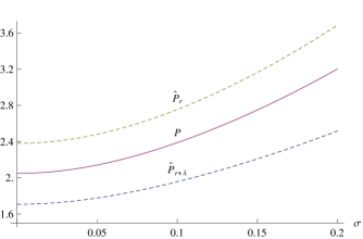
Figure 1: The impact of volatility on the option multipliers $P$, $\hat{P}_{r+\lambda}$, and $\hat{P}_{r}$

As Figure 1 indicates, the option multipliers are increasing as functions of the underlying volatility coefficient. Moreover, the option multipliers satisfies the condition $P\in(\hat{P}_{r+\lambda},\hat{P}_{r})$ as was established in our Theorem 3.2. The values of the optimal stopping problems are graphically illustrated for $\textrm{Beta}(c,d)$-distributed jumps in Figure 2 under the assumption that $\alpha=0.025,r=0.05,\lambda=0.02,a=b=K=1,c=1.25,d=5$, and $\sigma=0.1$ (which implies that $x^{\ast}=P=2.39,x^{\ast}_{0.07}=\hat{P}_{0.07}=1.96$, and $x^{\ast}_{0.05}=\hat{P}_{0.05}=2.75$)

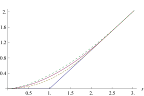
Figure 2: The exercise payoff $(x-1)^{+}$ and the values $V_{\lambda}(x),\tilde{V}_{r}(x),$ and $\tilde{V}_{r+\lambda}(x)$

Figure 2 illustrates explicitly the results of our Theorem 3.2 for the values of the stopping problems. It is of interest to notice that as was predicted by Theorem 3.2, the value $V_{\lambda}(x)$ of the considered stopping problem is sandwiched between the two values $\tilde{V}_{r+\lambda}(x)$ and $\tilde{V}_{r}(x)$.

It is worth noticing that in the present example the maximizing threshold $x^{\ast}$ exists even in cases where $k_{1}<1$, that is, even when the fundamental solution is not convex as a function of the state. Hence, for the considered exercise payoff the condition $r>\alpha$ guaranteeing the convexity of $x^{k_{1}}$ can be relaxed. If $0<r\leq\alpha$ then $k_{1}\in(0,1]$. Under those circumstances the sign of the relationship between increased volatility and the optimal exercise strategy is reversed as the root $k_{1}$ becomes an increasing function of volatility. More precisely, if $r\leq\alpha$ then $\partial x^{\ast}/\partial\sigma=-(x^{\ast}/k_{1}^{2})\partial k_{1}/\partial\sigma<0$ and $\partial x^{\ast}/\partial\lambda=-(x^{\ast}/k_{1}^{2})\partial k_{1}/\partial\lambda<0$. We illustrate this observation graphically for $\textrm{Beta}(c,d)$-distributed jumps in Figure 3 under the assumption that $\alpha=0.04,r=0.02,\lambda=0.01,a=K=1,b=0.2,c=1.25$, and $d=2$.

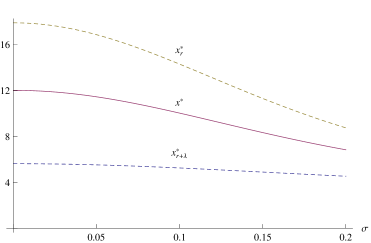
Figure 3: The impact of volatility on the exercise thresholds

Figure 3 illustrates how the sign of the relationship between increased volatility and the optimal exercise threshold is reversed as the increasing fundamental solution becomes concave. It is worth noticing that even in this case the order of the exercise thresholds remain naturally unchanged since the ordering of the values $V_{\lambda}(x)$, $\tilde{V}_{r+\lambda}(x)$, and $\tilde{V}_{r}(x)$ is based only on nonnegativity and monotonicity.

8 Conclusions

In this study we generalized a representation result known to hold for continuous linear diffusions to include a class of spectrally one-sided Lévy diffusions: given some conditions, the optimal stopping problem for a one-dimensional spectrally negative Lévy diffusion can be reduced to an ordinary nonlinear programming problem.

Considering the fact that optimal stopping problems feature prominently in pricing of American options and in real options theory, reducing the stopping problem of a Lévy diffusion into a standard programming problem can significantly facilitate the ongoing research on these areas of mathematical finance. We demonstrated this by deriving several interesting comparative static properties of spectrally negative Lévy diffusions using our representation, and found out that a useful tool in obtaining bounds for the value of the optimal stopping of a Lévy diffusion is the corresponding stopping problem for an associated continuous diffusion. By choosing the discount rates appropriately, we were able to sandwich the value of the considered optimal stopping problem between the known values of two stopping problems of the associated continuous diffusion.

Our study indicates that the impact of volatility on the optimal policy and its value in our setting is similar to the continuous case: for values convex (concave) below the optimal threshold, increased risk decelerates (accelerates) rational investment by expanding or leaving unchanged (shrinking or leaving unchanged) the continuation region and increasing or leaving unchanged (decreasing or leaving unchanged) the optimal threshold and the value of waiting. The impact of downside risk as measured by the intensity of the compound Poisson jump process on the optimal value was found out to be similar to the impact of the diffusion risk (as measured by the volatility). We also established that the key factor determining the relevant convexity/concavity properties of the value is (provided that it exists) the increasing fundamental solution of the associated integro-differential equation, which is process-specific. Thus we saw that the impact of volatility or downside risk is not dependent on the precise form of the exercise payoff, as long as the conditions for the optimality of the stopping rule characterized by a single threshold are met.

In addition to their usefulness in obtaining information about the comparative static properties of Lévy diffusions and their relations (similarities and differences) to the continuous diffusion case, our results raise an interesting question on the scope of applicability of our representation. This boils largely down to the question: when is the assumption on the existence of an increasing smooth solution to the characteristic integro-differential equation true, and can conveniently verifiable sufficient conditions for this be found? The technique developed in Rakkolainen, (2008) based on Frobenius series solutions appears to be a promising approach which may provide further insights into the considered class of problems.

Acknowledgments: The authors wish to thank Erik Baurdoux and Olli Wallin for their insightful comments. The financial support to Luis H. R. Alvarez E. from the OP Bank Research Foundation is gratefully acknowledged.

References

• Alvarez, (1996) Alvarez, L. H. R. Demand uncertainty and the value of supply opportunities, 1996, Z. Nationalökon. 64, 163–175.
• Alvarez, (2001) Alvarez, L. H. R. Reward functions, salvage values and optimal stopping, 2001, Math. Oper. Res. 54, 315–337.
• Alvarez, (2003) Alvarez, L. H. R. On the properties of r-excessive mappings for a class of diffusions, 2003, Ann. Appl. Probab. 13, 1517–1533.
• Alvarez, (2004) Alvarez, L. H. R.A class of solvable impulse control problems, 2004, Appl. Math. Optim. 49, 265–295.
• Alvarez, (2004) Alvarez, L. H. R. On risk adjusted valuation: A certainty equivalent characterization of a class of stochastic control problems, 2004, Discussion and working papers of Turku School of Economics and Business Administration, 5:2004.
• Alvarez and Rakkolainen, (2010) Alvarez, L. H. R., Rakkolainen, T. A. Investment timing in presence of downside risk: a certainty equivalent characterization, 2010, Ann. Finance, 6, 317–-333.
• Alvarez and Tourin, (1996) Alvarez, O., Tourin, A. Viscosity solutions of nonlinear integro-differential equations, 1996, Ann. Inst. H. Poincaré Anal. Non Linéaire. 13:3, 293–317.
• Alili and Kyprianou, (2005) Alili, L., Kyprianou, A. Some remarks on first passage of Lévy processes, the American put and pasting principles, 2005, Ann. Appl. Probab. 15:3, 2062–2080.
• Barles and Imbert, (2008) Barles, G., Imbert, C. Second-order elliptic integro-differential equations: viscosity solutions’ theory revisited, 2008, Ann. Inst. H. Poincaré Anal. Non Linéaire 25:3, 567–585.
• Beibel and Lerche, (1997) Beibel, M. and Lerche, H. R. A new look at optimal stopping problems related to mathematical finance, 1997, Statistica Sinica, 7, 93–108.
• Bernanke, (1983) Bernanke, B. S. Irreversibility, Uncertainty, and Cyclical Investment, 1983, Quart. J. Econ. 98:1, 85–103.
• Bertoin, (1996) Bertoin, J. Lévy processes, 1996, Cambridge University Press.
• Borodin and Salminen, (2002) Borodin, A. and Salminen, P.Handbook on Brownian motion - facts and formulae, 2002, 2nd ed. Birkhäuser, Basel.
• Boyarchenko, (2004) Boyarchenko, S. Irreversible decisions and record-setting news principles, 2004, Amer. Econ. Rev. 23:4, 557–568.
• Boyarchenko and Levendorskiĭ, (2002) Boyarchenko, S., Levendorskiĭ, S. Perpetual American options under Lévy processes, 2002, SIAM J. Control Optim. 40:6, 1663–1696.
• Boyarchenko and Levendorskiĭ, (2005) Boyarchenko, S., Levendorskiĭ, S. American options: the EPV pricing model, 2005, Ann. Finance 1:3, 267–292.
• Boyarchenko and Levendorskiĭ, (2007) Boyarchenko, S., Levendorskiĭ, S. Irreversible decisions under uncertainty. Optimal stopping made easy, 2007, Springer-Verlag.
• Casella and Berger, (2002) Casella, G., Berger, R. Statistical inference, 2002, Duxbury Press, 2nd edition.
• Cho and Stockbridge, (2002) Cho, M. J. and Stockbridge, R. S. Linear Programming Formulation for Optimal Stopping Problems, 2002, SIAM Journal on Control and Optimization, 40, 1965-–1982.
• Crandall et al., (1992) Crandall, M., Hitoshi, I., Lions, P. User’s guide to viscosity solutions of second order partial differential equations, 1992, Bull. Amer. Math. Soc. 27:1, 1–67.
• Dayanik and Karatzas, (2003) Dayanik, S., Karatzas, I. On the optimal stopping problem for one-dimensional diffusions, 2003, Stochastic Process. Appl. 107, 173–212.
• Dixit and Pindyck, (1994) Dixit, A. K. and Pindyck, R. S. Investment under uncertainty, 1994, Princeton UP, Princeton.
• Duffie et al, (2000) Duffie, D., Pan, J., Singleton, K. Transform analysis and asset pricing for affine jump diffusions, 2000, Econometrica 68:6, 1343–1376.
• Dynkin, (1965) Dynkin, E. B. Markov processes: volume II, 1965, Springer-Verlag, Berlin.
• Dynkin and Yuskevich, (1969) Dynkin, E. B., Yushkevich, A. A.Markov processes: theorems and problems, 1969, Plenum Press, New York.
• Gerber and Landry, (1998) Gerber, H., Landry, B. On the discounted penalty at ruin in a jump-diffusion and the perpetual put option, 1998, Ins.: Mathematics Econ. 22, 263–276.
• Gerber and Shiu, (1998) Gerber, H., Shiu, E. Pricing perpetual options for jump processes, 1998, N. Amer. Actuarial J. 2:3, 101–112.
• Helmes and Stockbridge, (2007) Helmes, K. and Stockbridge, R. S. Linear Programming Approach to the Optimal Stopping of Singular Stochastic Processes, 2007, Stochastics: An International Journal of Probability and Stochastic Processes, 79, 309–335.
• Hunt, (1958) Hunt, G. A. Markov processes and potentials I–III, 1957–58, Ill. J. Math. 1, 44–93 (I), 316–369 (II) , 2, 151–213 (III).
• Jakobsen and Karlsen, (2006) Jakobsen, E., Karlsen, K. A “maximum principle for semicontinuous functions“ applicable to integro-partial differential equations, 2006, NoDEA: Nonlinear differ. equ. appl. 13, 137–165.
• Karatzas and Shreve, (1999) Karatzas, I., Shreve, S. E. Methods of mathematical finance, 1999, Springer-Verlag.
• Kou and Wang, (2003) Kou, S. G., Wang, H. First passage times of a jump diffusion process, 2003, Advances in Applied Probability 35, 504–531.
• Kou, (2002) Kou, S. G. A jump diffusion model for option pricing, 2002, Management Science, 48, 1086–1101.
• Kyprianou, (2006) Kyprianou, A. E. Introductory lectures on fluctuations of Lévy processes with applications, 2006, Springer-Verlag.
• Lerche and Urusov, (2007) Lerche, H. R. and Urusov, M. Optimal stopping via measure transformation: The Beibel-Lerche approach, 2007, Stochastics, 3–4, 275–291.
• Mikosch, (2003) Mikosch, T. Modeling dependence and tails of financial time series, 2003, In: Finkenstaedt, B. and Rootzen, H. (2003) Extreme values in finance, telecommunications, and the environment. Chapman and Hall, 185–286.
• (37) Mordecki, E. Perpetual options for Lévy processes in the Bachelier model, 2002, Proc. Steklov Inst. Math. 237, 256–264.
• (38) Mordecki, E. Optimal stopping and perpetual options for Lévy processes, 2002, Finance Stoch. VI:4, 473–493.
• Mordecki and Salminen, (2007) Mordecki, E., Salminen, P. Optimal stopping of Hunt and Lévy processes, 2007, Stochastics 79(3-4), 233–251.
• Peskir, (2007) Peskir, G. A change-of-variable formula with local time on surfaces, 2007, In: Donati-Martin, C., Émery, M., Rouault, A., Stricker, C. Séminaire de Probabilités XL. Springer, 69–96.
• Peskir and Shiryaev, (2006) Peskir, G., Shiryaev, A. Optimal stopping and free-boundary problems, 2006, Birkhäuser.
• Pham, (1997) Pham, H. Optimal Stopping, Free Boundary, and American Option in a Jump-Diffusion Model, 1997, Applied Mathematics and Optimization, 35, 145–164.
• Protter, (2004) Protter, P. Stochastic integration and differential equations, 2004, Springer-Verlag, 2nd edition.
• Rakkolainen, (2008) Rakkolainen, T. A. A class of solvable Dirichlet problems associated to spectrally negative jump diffusions, 2008, working paper.
• Salminen, (1985) Salminen, P. Optimal stopping of one-dimensional diffusions, 1985, Math. Nachr. 124, 85–101.
• Øksendal, (2003) Øksendal, B. Stochastic differential equations. An introduction with applications, 2003, Springer-Verlag.
• Øksendal and Reikvam, (1998) Øksendal, B., Reikvam, K. Viscosity solutions of optimal stopping problems, 1998,Stoch. Stoch. Rep. 62, 285–301.
• Øksendal and Sulem, (2007) Øksendal, B., Sulem, A. Applied stochastic control of jump diffusions, 2nd edition, 2007, Springer-Verlag.