Data Placement and Replica Selection for Improving Co-location in Distributed Environments

Abstract

Increasing need for large-scale data analytics in a number of application domains has led to a dramatic rise in the number of distributed data management systems, both parallel relational databases, and systems that support alternative frameworks like MapReduce. There is thus an increasing contention on scarce data center resources like network bandwidth (especially cross-rack bandwidth); further, the energy requirements for powering the computing equipment are also growing dramatically. As we show empirically, increasing the execution parallelism by spreading out data across a large number of machines may achieve the intended goal of decreasing query latencies, but in most cases, may increase the total resource and energy consumption significantly. For many analytical workloads, however, minimizing query latencies is often not critical; in such scenarios, we argue that we should instead focus on minimizing the average query span, i.e., the average number of machines that are involved in processing of a query, through co-location of data items that are frequently accessed together. In this work, we exploit the fact that most distributed environments need to use replication for fault tolerance, and we devise workload-driven replica selection and placement algorithms that attempt to minimize the average query span. We model a historical query workload trace as a hypergraph over a set of data items (which could be relation partitions, or file chunks), and formulate and analyze the problem of replica placement by drawing connections to several well-studied graph theoretic concepts. We use these connections to develop a series of algorithms to decide which data items to replicate, and where to place the replicas. We show effectiveness of our proposed approach by building a trace-driven simulation framework and by presenting results on a collection of synthetic and real workloads. Our experiments show that careful data placement and replication can dramatically reduce the average query spans resulting in significant reductions in the resource consumption.

1 Introduction

Massive amounts of data are being generated every day in a variety of domains ranging from scientific applications to social networks to retail. The stores of data on which modern businesses rely are already vast and increasing at an unprecedented pace. Organizations are capturing data at deeper levels of detail and keeping more history than before. This deluge of data has led to a rapidly increasing use of parallel and distributed data management systems like parallel databases and MapReduce frameworks like Hadoop, to analyze and gain insights from the data. A variety of complex analysis tasks and queries are executed using these data management systems. In parallel databases, the queries typically consist of multiple joins, group-bys on multiple attributes, and complex aggregations. On Hadoop, the tasks often have similar flavor, with simplest of map-reduce programs being aggregation tasks that form the basis of analysis queries. There have also been many attempts to combine the scalability of Hadoop and declarative querying abilities of relational databases [40, 34].

Use of such parallel or distributed frameworks is expected to accelerate in the coming years, putting further strain on already-scarce resource like compute power, network bandwidth, and energy. For reducing total execution times, there is a trend towards increasing the execution parallelism by spreading out data across a large number of machines. However, this often increases the total resource consumption significantly, as we also illustrate empirically below. We argue that, for most analytical workloads, minimizing the query latencies may not be critically important since the queries are often not run in an interactive mode. Instead, we argue that we should aim for reducing the total resource consumption by decreasing the degree of single-query execution parallelism, i.e., by trying to reduce the number of machines involved in the execution of a query (called query span). There are several advantages to doing that:

Figure 1: Increasing the degree of parallelism may result in lower execution times, but leads to significantly higher resource and energy consumption.

Minimize the communication overhead: Query span directly impacts the total communication that must be performed to execute a query. This is clearly a concern in distributed setups (e.g., grid systems [39] or multi-datacenter deployments); however even within a data center, communication network is oversubscribed, and especially cross-rack communication bandwidth can be a bottleneck [22, 10]. In cloud computing, the total communication directly impacts the total dollar cost of executing a query. HDFS, for instance, tries to place all replicas of a data item in a single rack to minimize inter-rack data transfers [44]. We take this further, and argue for clustering replicas of different data items together to improve network performance for queries that access multiple data items.

Minimize the total amount of resources consumed: It is well-known that parallelism comes with significant startup and coordination overheads, and we typically see sub-linear speedups as a result of these overheads and data skew [35]. Although the response time of a query usually decreases in a parallel setting, the total amount of resources consumed typically increases with increased parallelism. Even in scenarios where we obtain super-linear speedups due to higher aggregate memory across the machines, we expect the total energy consumption to increase with the degree of parallelism.

Reduce the energy footprint: Computing equipment in US costs data center operators millions of dollars annually for energy, and also impacts the environment. Energy costs are ever increasing and hardware costs are decreasing – as a result soon the energy costs to operate and cool a data center may exceed the cost of the hardware itself. Minimizing the total amount of resources consumed directly reduces the total energy consumption of the task.

Illustrative Experiments: To support these claims and to motivate query span as a key metric to optimize, we conducted a set of experiments analyzing the effect of query span on the total resource and energy consumption under a variety of settings. First setting is a horizontally partitioned MySQL cluster, on which we execute four SQL queries against a TPC-H database. Two of the queries are complex analytical join queries (TPC-H1, TPC-H2 in Figure 1), whereas the other two are simple aggregation queries on a single table (TPC-H3, TPC-H4). In the second setting, we implemented our own distributed query processor on the top of multiple MySQL instances running on a cluster where predicate evaluations are pushed on to the individual nodes and data is shipped to a single node for perform the final steps. On this setup we evaluate two queries: a complex join query (Q-Join) and a simple aggregate query on a single table (Q-Sum). In Figures 1 and 1, we plot the execution times and the energy consumed as the number of machines across which the tables are partitioned (and hence query span) increases. The energy consumption is estimated by using an Itanium server power model constructed by using the Mantis full-system power modelling technique [15]. We use the dstat tool to collect various system performance counters such as CPU utilization, network reads and writes, I/O, and memory footprint, and then use the power model to estimate the total energy consumed.

As we can see, the execution times of the TPC-H queries run on MySQL cluster actually increased with parallelism, which may be because of nested loop join implementation in MySQL cluster (a known problem that is being fixed). In our implementation, the execution time remains constant. But in all cases, energy consumption increased with query span. In the second experiment with simpler queries (Figures 1 and 1), though execution times decrease as the query span increases, energy consumption increases in all cases. From this simple set of experiments it is evident that, as the number of machines involved in processing a query increases, total resources consumed to process the query also rise.

Goals and Contributions: In this paper, we propose a workload-driven approach that aims to reduce the average query span in distributed data management systems by co-locating data items that are frequently accessed together by queries. We observe that, for fault tolerance, load balancing, and availability, those systems typically maintain several copies of each data item (e.g., Hadoop file system (HDFS) maintains at least 3 copies of each data item by default [44]), and we propose exploiting this inherent replication to achieve higher co-location by judicious replica creation and placement. Our approach is workload-driven in that, we propose capturing a historical query workload over a period of time, and optimizing data placement and replication for that workload. Our techniques work on an abstract representation of the query workload, and are applicable to both multi-site data warehouses and general purpose data centers. We represent the query workload as a hypergraph, where the nodes are the data items and each query is translated into a hyperedge over the nodes. The data items could be database relations, parts of database relations (e.g., tuples or columns), or arbitrary files. The goal is to store each data item (node in the graph) onto a subset of machines/sites (also called partitions), obeying the storage capacity requirements for the partitions. Note that the partitions do not have to be machines, but could instead represent racks or even datacenters. The span of a query is defined to be the smallest number of partitions that contain all the data that the query needs. Our goal is to find a layout that minimizes the average span over all queries in the workload. Further, our algorithms can optimize for load or storage constraints, or both.

Our key contributions include formulating and analyzing this problem, drawing connections to several problems studied in the graph algorithms literature, and developing efficient algorithms for data placement. In addition, we examine the special case when each query accesses at most two data items – in this case the hypergraph is simply a graph. For this case, we are able to develop theoretical bounds for special classes of graphs that gives an understanding of the trade-off between energy cost and storage. We have also built a trace-driven simulation framework that enables us to systematically compare different algorithms, by automatically generating varying types of query workloads and by calculating the total energy cost of a query trace. We conducted an extensive experimental evaluation using our framework, and our results show that our techniques can result in high reductions in query spans and resource consumption compared to baseline or random data placement approaches.

Discussion: Making data placement and replication decisions with the goal of minimizing average query spans raises several concerns. First, as discussed above, it may increase the execution time of a single query, and hence such an approach can only be used if the workload is not latency-sensitive. We argue that an increasing number of analytical workloads, especially those primarily consisting of batch analysis tasks, fall in that category. If the primary goal is to minimize the query response time, then declustering should instead be utilized to leverage the parallelism by spreading out the data items. Second, focusing simply on minimizing query spans can lead to a load imbalance across the partitions. There are two ways this could be handled. We can use temporal scheduling (by postponing certain queries) to balance loads across machines. We can also easily modify our algorithms to incorporate load constraints. A third concern is the cost of replica maintenance. However, most distributed systems do replication for fault tolerance, and hence our approach does not add a significant extra overhead. Further, most systems geared towards large-scale analytics perform batch updates, and the overall cost of updates is relatively low. Finally, like any workload-driven approach, our proposed approach relies on the ability to capture and model an expected query workload. With increasing automation in data analysis, with the same queries or analysis tasks being run on a regular basis, we believe this is a reasonable assumption to make.

Our proposed techniques have broader applicability beyond the application domains that we discuss in this paper. We can use similar techniques to partition large graphs across a distributed cluster; smart replication of some of the (boundary) nodes can result in significant savings in the communication cost to answer queries [31]. Our techniques are also applicable in partition farms such as MAID [11], PDC [36], or Rabbit [6], that utilize a subset of a partition array as a workhorse to store popular data so that other partitions could be turned off or sent to lower energy modes. A recent system, CoHadoop [16], also aims at co-locating related data items to improve performance of Hadoop, and provides a lightweight mechanism that allows applications to control where data is stored. They focus on data co-location to improve the efficiency of many operations, including indexing, grouping, aggregation, columnar storage, joins, and sessionization. Our workload-driven techniques are complimentary to their work, and can be used to further guide the data placement decisions in their system.

In a recent work, Curino et al. [12] also proposed a workload-aware approach for database partitioning and replication to minimize the number of sites involved in distributed transactions. They however do not develop new partitioning techniques. Although there are superficial similarities in use of graph partitioning techniques, there are several major differences. First, the number of data items is significantly higher in that application domain (since the approach treats each tuple as a data item); second, we largely assume a read-only workload, but in their setting, replication costs must be taken into account. We note that, in a concurrent submission by a subset of the authors [37], we propose a suite of techniques for scalable workload-aware data partitioning and replication for OLTP workloads, that builds upon the work by Curino et al. Unlike this submission where the focus is on developing new partitioning and replication algorithms, in that work, our focus is on minimizing the partitioning and bookkeeping overheads, on minimizing update costs through use of quorums, and on handling dynamic changes to the workload through incremental re-partitioning.

Outline: We begin with a discussion of closely related work (Section 2). We formally define the problem that we address in the paper and analyze it (Section 3). We present a series of algorithms to solve the problem (Section 4), and present an extensive performance evaluation using real dataset on Amazon EC2 and trace-driven simulation framework that we have built (Section 5).

2 Related Work

Data partitioning and replication plays an increasingly important role in large scale distributed networks such as content delivery networks (CDN), distributed databases and distributed systems such as peer-to-peer networks. Due to space constraints, we limit our discussion to the most relevant work here, and refer to the extended version for further discussion [1]. Aside from CoHadoop work discussed above [16], Hadoop++ [13] is another closely related work that exploits data pre-partitioning and co-location. There is substantial amount of work on replica placement that focuses on minimization of network latency and bandwidth. Neves et al. [32] propose a technique for replication in CDN where they replicate data onto a subset of servers to handle requests so that the traffic cost in the network is minimized. There has been a lot of work on dynamic/adaptive replica management (e.g., [45]), where replicas are dynamically placed, moved, or deleted based on the read/write access frequencies of the data items again with the goal of minimizing bandwidth and access latency.

Graphs have been used as a tool to model various distributed storage problems and to come up with replication strategies to achieve a specific objective. Du et al. [14] study Quality-of-Service (QoS)-aware replica placement problem in a general graph model. In their model, vertices are the servers with various weights representing node characteristics and edges representing the communication costs. Other work has modeled network topology as a graph and developed replication strategies or approximations (replica placement in general graphs is NP-complete) [46]. In contrast, we model query workload as a hypergraph, and assume a uniform network topology (i.e., identical communication costs between any pair of nodes); we believe this better approximates the current networks.

Issues in energy-efficient computing are being increasingly studied at all layers of today’s computing infrastructures. Harizopoulos et al. [21] reported the first results on software-level optimizations to achieve better energy efficiency; they experiment with a system that was configured similarly to an audited TPC-H server and show that making the right physical design decisions can improve energy efficiency. Additionally, they use relational scan operator as a basis to demonstrate that optimizing for performance is different from optimizing for energy efficiency. It is also among the first papers [21, 20, 26] to practically show the importance of energy efficiency in database systems. Leverich et al. [28] and Lang et al. [27] suggest approaches to conserving energy by powering down Hadoop cluster nodes. Tsirogiannis et al. [43] analyze the energy efficiency of a single-node database server, and argue that the most energy-efficient configuration is typically the highest performing one. However, this assertion is valid only for single node database server, and does not hold for scale-out architectures involving multiple machines where parallelization, communication, and startup overheads come into play. From our experiments over the TPC-H benchmark, it is evident that, as the number of machines involved in processing a query increases, total resources consumed to process the query also rise.

Our work is different from several other works on data placement [25, 29, 33] where the database query workload is also modeled as a hypergraph and partitioning techniques are used to drive data placement decisions. Tosun et al. [41, 42] and Ferhatosmanoglu et al. [18] propose using replication along with declustering for achieving optimal parallel I/O for spatial range queries. The goal with all of that prior work is typically minimization of latencies and query response times by spreading out the work over a large number of partitions or devices. For us, that is exactly the wrong optimization goal – we would like to cluster data required for each query on as few partitions as possible.

The problems we study are closely related to several well-studied problems in graph theory and can be considered generalizations of those problems. A basic special case of our main problem is the minimum graph bisection problem (which is NP-Hard), where the goal is to partition the input graph into two equal sized partitions, while minimizing the number of edges that are cut [8]. There is much work on both that problem and its generalization to hypergraphs and to $k$-way partitioning [30, 23, 24]. Another closely related problem is that of finding dense subgraphs in a graph, where the goal is to find a group of vertices where the number of edges in the induced subgraph is maximized [17]. Finally, there is much work on finding small separators in graphs. Several theoretical results on known about this problem. We discuss these connections in more detail later when we describe our proposed algorithms.

3 Problem Definition; Analysis

Next, we formally define the problem that we study, and draw connections to some closely related prior work on graph algorithms. We also analyze a special case of the problem formally, and show an interesting theoretical result.

Problem Definition: Given a set of data items $\mathcal{D}$ and a set of partitions, our goal is to decide which data items to replicate and how to place them on the partitions to minimize the average span of an expected query workload; span of a query is defined to be the minimum number of partitions that must be accessed to answer the query. To make the problem more concrete, we assume that we are given a set of queries over the data items, and our goal is to minimize the average span over these queries. For simplicity, we assume that we are given a total of $N$ identical partitions each with capacity $C$ units, and further that the data items are all unit-sized (we will relax this assumption later). Clearly, the number of data items must be smaller than $N\times C$ (so that each data item can be placed on at least one partition). Further, let $N_{e}$ denote the minimum number of partitions needed to place the data items (i.e., $N_{e}=\lceil|\mathcal{D}|/C\rceil$).

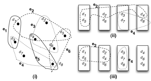
Figure 2: (i) Modeling a query workload as a hypergraph – $d_{i}$ denotes the data items, and $e_{i}$ denotes the queries represented as hyperedges; (ii) A layout w/o replication onto 4 partitions – the span of two of the hyperedges is also shown; (iii) A layout with replication – span for both queries reduces by 1.

The query workload can be represented as a hypergraph, $\mathcal{H}=(V,E)$, where the nodes are the data items and each (hyper)edge $e\in E$ corresponds to a query in the workload. Figure 2 shows an illustrative example, where we have 6 queries over 8 data items, each of which is represented as a hyperedge over the data items. The figure also shows two layouts of the data items onto 4 partitions of capacity 3 each, without replication and with replication.

Calculating Span: When there is no replication, calculating the span of a query is straightforward since each data item is associated with a single partition. However, if there is replication, the problem becomes NP-Hard. It is essentially identical to the minimum set cover problem [19], where we are given a collection of subsets of a set (in our case, the partitions) and a query subset, and we are asked to find the minimum number of subsets (partitions) required to cover the query subset.

As an example, for query $e_{2}$ in Figure 2, the span in the first layout is 3. However, in the second layout, we have to choose which of the two copies of $d_{4}$ to use for the query. Using the first copy (on second partition) leads to the lowest span of 2. Overall, the average query span for the first layout is $13\over 6$, but use of replication in the second layout reduces this to $8\over 6$.

We use a standard greedy algorithm for choosing replicas to use for a query and for calculating the span. For each of the partitions, we compute the size of its intersection with the query subset. We choose the partition with the highest intersection size, remove all items from the query subset that are contained in the partition, and iterate until there are no items left in the query subset. This simple greedy algorithm provides the best known approximation to the set cover problem ($\log|Q|$, where $|Q|$ is the query size).

Hypergraph Partitioning: Without replication, the problem we defined above is essentially the $k$-way (balanced) hypergraph partitioning problem that has been very well-studied in the literature. However, the optimization goal of minimizing the average span is unique to this setting; prior work has typically studied how to minimize the number of cut hyperedges instead. Several packages are available for partitioning very large hypergraphs efficiently [2, 3]. The proposed algorithms are typically heuristics or combinations of heuristics, and most often the source code is not available. We use one such package (hMETIS) as the basis of our algorithms.

Finding Dense Subgraphs of a specified size: Given a set of nodes $S$ in a graph, the density of the subgraph induced by $S$ is defined to be the ratio of the number of edges in the induced subgraph and $|S|$. The dense subgraph problem is to find the densest subgraph of a given size. To understand the connection to the dense subgraph problem, consider a scenario where we have exactly one “extra” partition for replicating the data items (i.e., $N_{e}=N-1$). Further, assume that each query refers to exactly two data items, i.e., the hypergraph $\mathcal{H}$ is just a graph. One approach would then be to first partition the data items into $N-1$ partitions without replication, and then try to use this extra partition optimally. To do this, we can construct a residual graph, which contains all edges that were cut in this partitioning. The span of each of the queries corresponding to these edges is exactly 2. Now, we find the subgraph of size $C$ such that the number of induced edges (among the nodes of the subgraph) is maximized, and we place these data items on the extra partition. The span of the queries corresponding to these edges are all reduced from 2 to 1, and hence this is an optimal way to utilize the extra partition. We can generalize this intuition to hypergraphs and this forms the basis of one of our algorithms.

Unfortunately, the problem of finding the most dense subgraph of a specified size is NP-Hard (with no good worst case approximation guarantees), so we have to resort to heuristics. One such heuristic that we adapt in our work is as follows: recursively remove the lowest degree node from the residual graph (and all its incident edges) till the size of the residual graph is exactly $C$. This heuristic has been analysed by Asahiro et al. [7] who find that this simple greedy algorithm can solve this problem with approximation ratio of approximately $2(\frac{|V|}{C}-1)$ (when $C\leq|V|/3$).

Sublinear Separators in Graphs: Consider the special case where $\mathcal{H}$ is a graph, and further assume that there are only 2 partitions (i.e., $N=2$). Further, lets say that the graph has a small separator, i.e., a set of nodes whose deletion results in two connected components of size at most $n/2$. In that case, we can replicate the separator nodes (assuming there is enough redundancy) and thus guarantee that each query has span exactly 1. The key here is the existence of small separators of bounded sizes. Such separators are known to exist for many classes of graphs, e.g., for any family of graphs that excludes a minor [4].

A separator theorem is usually of the form that, any $n$-vertex graph can be partitioned into two sets $A$, $B$, such that $|A\cap B|=c\sqrt{n}$ for some constant $c$, $|A-B|<2n/3$, $|B-A|<2n/3$, and there are no edges from a node in $A-B$ to a node in $B-A$. This directly suggests an algorithm that recursively applies the separator theorem to find a partitioning of the graph into as many pieces as required, replicating the separator nodes to minimize the average span. Such an algorithm is unlikely to be feasible in practice, but may be used to obtain theoretical bounds or approximation algorithms. For example, we prove that:

Theorem 1

Let $G$ be a graph with $n$ nodes that excludes a minor of constant size. Further, let $N_{e}$ denote the number of partitions minimally required to hold the nodes of $G$ (i.e., $N_{e}=\lceil n/C\rceil$). Then, asymptotically, $N_{e}^{1.73}$ partitions are enough to partition the nodes of $G$ with replication so that each edge is contained completely in at least one partition.

For general graphs, we show that:

Theorem 2

If the optimal solution uses $\beta N_{e}$ partitions to place the data items so that each edge is contained in at least one partition, then either we can get an approximation with factor $\frac{2}{2-\alpha}$ for $0\leq\alpha\leq 1$ using $N_{e}$ partitions, or a placement using $\frac{CN_{e}\beta}{2\alpha}$ partitions with span 1 for each edge.

Proofs of both the theorems can be found in the extended version of the paper [1].

4 Data Placement Algorithms

In this section, we present several algorithms for data placement with replication, with the goal to minimize the average query span. Instead of starting from scratch, we chose to base our algorithms on existing hypergraph partitioning packages. As we discussed in the previous sections, the problem of balanced and unbalanced hypergraph partitioning has received a tremendous amount of attention in various communities, especially the VLSI community. Several very good packages are freely available for solving large partitioning problems [2, 23, 3, 9]. We use a hypergraph partitioning algorithm (called HPA) as a blackbox in our algorithms, and focus on replicating data items appropriately to reduce the average query span. An HPA algorithm typically tries to find a balanced partitioning (i.e., all partitions are of approximately equal size) that minimizes some optimization goal. Usually, allowing for unbalanced partitions results in better partitioning. In the algorithm descriptions below, we assume that the HPA algorithm can return an exactly balanced partition, where all partitions are of equal size, if needed.

Following the discussion in the previous section, we develop four classes of algorithms:

• Iterative HPA (IHPA): Here we repeatedly use HPA until all the extra space is utilized.

• Dense Subgraph-based (DS): Here we use a dense subgraph finding algorithm to utilize the redundancy.

• Pre-replication (PR): Here we attempt to identify a set of nodes to replicate a priori, modify the input graph by replicating those nodes, and then run HPA to get a final placement.

• Local Move-based (LM): Starting with a partition returned by HPA, we improve it by replicating a small group of data items at a time.

As expected the space of different variants of the above algorithms is very large. We experimented with many such variants in our work. We begin with a brief listing of some of the key subroutines that we use in the pseudocodes. We then describe a representative set of algorithms that we use in our performance evaluation.

4.1 Preliminaries; Subroutines

The inputs to the data placement algorithm are: (1) the hypergraph, $\mathcal{H}(V,E)$, with vertex set $V$ and (hyper)edge set $E$ that captures the query workload, and (2) the number of partitions, $N$ and (3) the capacity of each partition $C$. We use $N_{e}$ to denote the minimum number of partitions needed to partition the hypergraph ($N_{e}\leq N$).

Our algorithms use a hypergraph partitioning algorithm (HPA) as a blackbox. HPA takes as input the hypergraph to be partitioned, the number of partitions, and an unbalance factor (UBfactor). The unbalance factor is set so that HPA has the maximum freedom, but the number of nodes placed in any partition does not exceed $C$. For instance, if $|V|=N_{e}\times C$ and if HPA is asked to partition into $N_{e}$ partitions, then the unbalance factor is set to be the minimum. However, if HPA is called with $N^{\prime}>N_{e}$ partitions, then we appropriately set the unbalance factor to the maximum possible. The formula we use in our experiments to set unbalance factor is:

$$UBfactor=100*\frac{partitionCapacity*noPartitions-totalItems}{totalItems*noPartitions}$$

We modify the output of HPA slightly to ensure that the partition capacity constraints are not violated. This is done as follows: if there is a partition that has higher than maximum number of nodes, we move a small group of nodes to another partition with fewer than maximum number of nodes. We use one of our algorithms developed below (LMBR) for this purpose.

In the pseudocodes shown, apart from HPA, we also assume existence of the following subroutines:

• avgDataItemsPerQuery$(\mathcal{H})$: Suppose $V_{i}$ is the set of data items covered by hyperedge $e_{i}\in\mathcal{H}$. The $\Sigma_{e_{i}\in\mathcal{H}}|V_{i}|$ gives the average number of data items covered per query.

• getSpanningPartitions($\mathcal{G},e$): Let the current placement (during the course of the algorithm) be $\mathcal{G}=\{G_{1},\cdots,G_{N}\}$ where $G_{1},\cdots,G_{n}$ denote the subgraphs of $\mathcal{G}$ assigned to the different partitions and may not be disjoint (i.e., same node may be contained in two or more partitions because of replication). Given a hyperedge $e$, this procedure finds a minimal subset of the partitions $MD_{e}\subseteq\mathcal{G}$, such that every node in $e$ is contained in at least one partition in $MD_{e}$. We use the greedy Set Cover algorithm for this purpose. We start with the partition $G_{i}$ that has the maximum overlap with $e$, and include it in $MD_{e}$. We then remove all the nodes in $e$ that are contained in $G_{i}$ (i.e., “covered” by $G_{i}$) and repeat till all nodes are covered.

• getQuerySpan($\mathcal{G},e$): Given a current placement $\{G_{1},\cdots,G_{N}\}$ and a hyperedge $e$, this procedure finds the span of the hyperedge $e$. We use the same algorithm as above, but return $|MD_{e}|$ instead of $MD_{e}$.

• getAccessedItems($\mathcal{G},e,g\in\mathcal{G}$): Given a current placement $\mathcal{G}=\{G_{1},\cdots,G_{N}\}$, a hyperedge $e$ and a partition $g\in\mathcal{G}$, this returns the set of items that the query corresponding to $e$ would access from partition $g$, as computed by the greedy Set Cover algorithm. This may be empty even if $e\cap g\neq\phi$.

• pruneHypergraphBySpan($\mathcal{G},\mathcal{H},minSpan$): Given a current placement $\mathcal{G}$ and a value of $minSpan$, this routine removes all hyperedges from $\mathcal{H}$ with span less than or equal to $minSpan$.

• getKDensestNodes($\mathcal{H},K$): Given a hypergraph $\mathcal{H}$, this procedure returns a dense subgraph containing at nodes having total weight of atmost $K$. We use a greedy algorithm for this purpose: we find the lowest degree node and remove that node and all edges incident on it; if the graph still has nodes having total weight more than $K$, we repeat the process by finding the lowest degree node in the new graph.

• pruneHypergraphToSize($\mathcal{H},K$): Given a current placement $\mathcal{G}$ and a value of $K$, this routine uses the same algorithm as for getKDensestNodes to find a (dense) hypergraph over nodes having total weight of $K$.

• totalWeight($V$, $W_{v}$): Given a set of vertices $V$ and weight vector of vertices $W_{v},v\in V$, this routine returns the total weight of vertices.

We note that, because of the modularized way our framework is designed, we can easily use different, more efficient algorithms for solving these subproblems.

4.2 Iterative HPA (IHPA)

Here, we start by using HPA to get a partitioning of the data items into exactly $N_{e}$ partitions (recall that $N_{e}$ is the minimum number of partitions needed to store the data items). We then prune the original hypergraph $\mathcal{H}(V,E)$ to get a residual hypergraph $\mathcal{H}^{{}^{\prime}}(V^{{}^{\prime}},E^{{}^{\prime}})$ as follows: we remove all hyperedges that are completely contained in a single partition (i.e., hyperedges with span 1), and we then remove all the data items that are not contained in any hyperedge. If the number of nodes in the $\mathcal{H}^{\prime}$ is less than $(N-N_{e})C$ (i.e., if the data items fit in the remaining empty partitions), we apply HPA to obtain a balanced partitioning of $\mathcal{H}^{\prime}$ and place the partitions on the remaining partitions. This process is repeated if there are still empty partitions.

If the number of nodes in $\mathcal{H}^{\prime}$ is larger than the remaining capacity, we prune the graph further by removing the hyperedges with the lowest span one at a time (these hyperedges are likely to see the least improvement by replication) and the data items that now have 0 degree, until the number of nodes in $\mathcal{H}^{\prime}$ becomes sufficiently low; then we apply HPA to obtain a balanced partitioning of $\mathcal{H}^{\prime}$ and place the partitions on the remaining partitions. If there are still empty partitions, we repeat the process by reconstructing a new residual graph. Algorithm 1 depicts the pseudocode for this technique.

Algorithm 1 Iterative HPA (IHPA)

0:  $\mathcal{H}(V,E),N,C$

1:  Run HPA to get an initial partitioning into $N_{e}$ partitions: $\mathcal{G}=\{G_{1},G_{2},\dots,G_{N_{e}}\}$;

2:  $edgeCost=$ avgDataItemsPerQuery$(\mathcal{H})$;

3:  while $edgeCost\neq 0$ and $|\mathcal{G}|\neq N$ do

4:     $\mathcal{H}^{{}^{\prime}}(V^{\prime},E^{\prime})=$ pruneHypergraphBySpan$(\mathcal{G},\mathcal{H},edgeCost)$;

5:     $N_{cur}=\frac{totalWeight(V^{{}^{\prime}},W_{v^{\prime}})}{C}$;

6:     if $|\mathcal{G}|+N_{cur}\leq N$ and $|\mathcal{H^{{}^{\prime}}}|\neq 0$ then

7:        $\mathcal{G}$ = $\mathcal{G}$ $\cup$ HPA$(\mathcal{H^{{}^{\prime}}},N_{cur})$;

8:     else if $|\mathcal{G}|+N_{cur}>N$ then

9:        $\mathcal{G}$ = $\mathcal{G}$ $\cup$ HPA$(\mathcal{H^{{}^{\prime}}},N-|\mathcal{G}|)$;

10:     else

11:        decrement $edgeCost$ by 1;

12:     end if

13:  end while

14:  return  final partitions $G_{1},G_{2},\cdots,G_{N}$

4.3 Dense Subgraph-based (DS)

This algorithm directly follows from the discussion in the previous section. As above, we use HPA to get an initial partitioning. We then fill the remaining $N-N_{e}$ partitions one at a time, by identifying a dense subgraph of the residual hypergraph. This is done by removing the lowest degree nodes from $\mathcal{H}^{\prime}$ until the number of nodes in it reaches $C$ (the partition capacity). These data items are then placed on one of the remaining partitions, and the procedure is repeated until all partitions are utilized. Pseudocode is shown in Algorithm 2.

Algorithm 2 Dense Subgraph-based (DS)

0:  $\mathcal{H}(V,E),N,C$

1:  Run HPA to get an initial partitioning into $N_{e}$ partitions: $\mathcal{G}=\{G_{1},G_{2},\dots,G_{N_{e}}\}$;

2:  $\mathcal{H^{{}^{\prime}}}=\mathcal{H}$;

3:  while $|\mathcal{G}|\neq N$ do

4:     $\mathcal{H^{{}^{\prime}}}=$ pruneHypergraphBySpan$(\mathcal{G},\mathcal{H},1)$;

5:     if $|\mathcal{H}^{\prime}|=0$ then

6:        break;

7:     end if

8:     $denseNodes$ = getKDensestNodes$(\mathcal{H^{{}^{\prime}}},C)$;

9:     Add a partition containing $denseNodes$ to $\mathcal{G}$;

10:  end while

11:  return  final partitions $G_{1},G_{2},\cdots,G_{N}$

4.4 Pre-Replication-based Algorithm (PRA)

This algorithm is based on the idea of identifying small separators and replicating them. However, we do not directly adapt the recursive algorithm described in Section 3 for two reasons. First, since we have a fixed space budget for replication, we must somehow distribute this budget to the various stages and it is unclear how to do that effectively. More importantly, the basic algorithm of bisecting a graph and then recursing is not considered a good approach for achieving good partitioning [38, 24].

We instead propose the following algorithm. We start with a partitioning returned by HPA, and identify “important” nodes such that by replicating these nodes, the average query span would be reduced the most. Then, we create a new hypergraph by replicating these nodes (until we have enough nodes to fill all the partitions), and run HPA once again to attain a final partitioning. However, neither of these steps is straightforward.

Identifying Important Nodes: The goal is to decide which nodes will offer the most benefit if replicated. We start with a partitioning obtained using HPA, and then analyze the partitions to decide this. We describe the intuition first. Consider a node $a$ that belongs to some partition $G_{i}$. Now count the number of those hyperedges that contain $a$ but do not contain any other node in $G_{i}$; we denote this number by $score_{a}$. If this number is high, then the node is a good candidate for replication since replicating the node is likely to reduce the query spans for several queries. We use the partitioning returned by HPA to rank all the nodes in the decreasing order by this count, and then process the nodes one at a time.

Algorithm 3 Pre-replication-based Algorithm (PRA)

0:  $\mathcal{H}(V,E),N,C$

1:  Run HPA to get an initial partitioning into $N_{e}$ partitions: $\mathcal{G}=\{G_{1},G_{2},\dots,G_{N_{e}}\}$;

2:  for $v\in V$ do

3:     let $v$ be contained in partition $G_{v}$;

4:     compute $score_{v}=|\{e\in E\ |\ e\cap G_{v}=\{v\}\}|$;

5:  end for

6:  $H^{r}=H$;

7:  for $v\in V$ in decreasing order by $score_{v}$ do

8:     $E_{v}=\{e\in E\ |\ v\in e\}$;

9:     $G_{v}=\{$getSpanningPartitions$(\mathcal{G},e)\ |\ e\in E_{v}\}$;

10:     $S=$ getHittingSet$(G_{v})$;

11:     for $g\in S$ do

12:        $copy_{g}=$ makeNewCopy$(v)$;

13:        for $e\in E_{v}$ s.t. $g\in$getSpanningPartitions$(\mathcal{G},e)$ do

14:           $e=e-\{v\}+\{copy_{g}\}$;

15:        end for

16:     end for

17:  end for

18:  $\mathcal{G}=$ HPA$(\mathcal{H}^{r},N)$;

19:  return  final partitions $G_{1},\cdots,G_{N}$

Replicating Important Nodes: Let $d$ be the node with the highest value of $score_{d}$ among all nodes. We now have to decide how many copies of $d$ to create, and more importantly, which copies to assign to which hyperedge. Figure 3(ii) illustrates the problems with an arbitrary assignment. Here we replicate the node $d$ to get one more copy $d^{\prime}$, and then we assign these two copies to the hyperedges $e_{1},e_{2},e_{3},e_{4}$ as shown (i.e., we modify some of the hyperedges to remove $d$ and add $d^{\prime}$ instead). However, the assignment shown is not a good one for a somewhat subtle reason. Since $e_{1}$ and $e_{3}$ (which are assigned the original $d$) do not share any other nodes, it is likely that they will span different sets of partitions, and one of them is likely to still pay a penalty for node $d$. On the other hand, the assignment shown in Figure 3(iii) is better because here the copies are assigned in a way that would reduce the average query span.

We formalize this intuition in the following algorithm. For node $d$, let $E_{d}=\{e_{d_{1}},e_{d_{2}},\cdots,e_{d_{k}}\}$ denote the set of hyperedges that contain $d$. For hyperedge $e_{d_{i}}$, let $\mathcal{G}_{d_{i}}$ denote the set of partitions that $e_{d_{i}}$ spans. We then identify a set of partitions, $S$, such that each of $\mathcal{G}_{d_{i}}$ contains at least one partition from this set (i.e., $S\cap\mathcal{G}_{d_{i}}\neq\phi$). Such a set is called a “hitting set”. We then replicate $d$ to make a total of $|S|$ copies. Finally, we assign the copies to the hyperedges according to the hitting set, i.e., we uniquely associate the copies of $d$ with the members of $S$, and for a hyperedge $e_{d_{i}}$, we assign it a copy such that the associated element from $S$ is contained in $\mathcal{G}_{d_{i}}$ (if there are multiple such elements, we choose one arbitrarily).

The problem of finding the smallest hitting set is NP-Hard. We use a simple greedy heuristic. We find the partition that is common to the maximum number of sets $\mathcal{G}_{d_{i}}$, include it in the hitting set, remove all sets that contain it, and repeat. Algorithm 3 depicts the pseudocode for this technique.

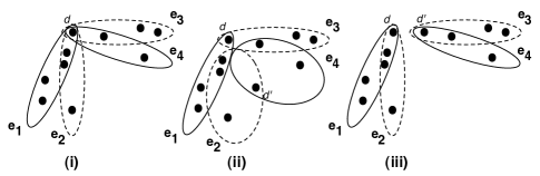
Figure 3: When replicating a node, distribution of the copies to the hyperedges must be done carefully. Distribute the replica copies such that it results in entanglement of the incident hyperedges.

4.5 Local Move Based Replication (LMBR)

Finally, we consider algorithms based on local greedy decisions about what to replicate, starting with a partitioning returned by HPA. For simplicity and efficiency, we chose to employ moves involving two partitions. More specifically, at each step, we copy a small group of data items from one partition to another. The decisions are made greedily by finding the move that results in the highest decrease in the average query span (“benefit”) per data item copied (“cost”). For this purpose, at all times, we maintain a priority queue containing the best moves from $partition_{i}$ to $partition_{j}$, for all $i\neq j$. For two partitions $partition_{i},partition_{j}$, the best group of data items to be copied from $partition_{i}$ to $partition_{j}$ is calculated as follows. Let $E_{ij}=\{e_{{ij}_{1}},\cdots,e_{{ij}_{l}}\}$ denote the hyperedges that contain data items from both the partitions. We construct a hypergraph $H_{i\rightarrow j}$ on the data items of $partition_{i}$ as follows: for every edge $e_{{ij}_{k}}$, we add a hyperedge to $H_{i\rightarrow j}$ on the data items common to $e_{{ij}_{k}}$ and $partition_{i}$. Figure 4 illustrates this process with an example.

Now, if we were to copy a group of data items $X$ from $partition_{i}$ to $partition_{j}$, the resulting decrease in total span (across all edges) is exactly the number of hyperedges in $H_{i\rightarrow j}$ that are completely contained in $X$. Thus, the problem of finding the best move from $partition_{i}$ to $partition_{j}$ is similar to the problem of finding a dense subgraph, with the main difference being that, we want to minimize the cost/benefit ratio and not maximize the benefit alone. Hence, we modify the algorithm for finding dense subgraph as follows. We first compute the cost/benefit ratio for the entire group of nodes in $H_{i\rightarrow j}$. The cost is set to $\infty$ if the number of nodes to be copied is more than the empty space in $partition_{j}$. We then remove the lowest degree node from $H_{i\rightarrow j}$ (and any incident hyperedges), and again compute the cost/benefit ratio. We pick the group of items that results in the lowest cost/benefit ratio.

After finding the best moves for every pair of partitions, we choose the overall best move, and copy the data items accordingly. We then recompute the best moves for those pairs which were affected by this move (i.e., the pairs containing the destination partition), and recurse until all the partitions are full.

Improved LMBR: Although the above looks like a reasonable algorithm, it did not perform very well in our first set of experiments. As described above, the algorithm has a serious flaw. Going back to the example in Figure 4, say we chose to copy data item $d_{6}$ from $partition_{1}$ to $partition_{2}$. In the next step, the same move would still rank the highest. This is because the construction of hypergraph $H_{1\rightarrow 2}$ is oblivious to the fact that $d_{6}$ is also now present in $partition_{2}$. Further, it is also possible that, because of replication, neither of the partitions is actually accessed at all when executing the queries corresponding to $e_{4},e_{5}$ or $e_{6}$.

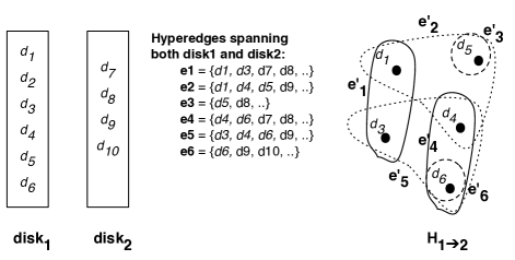
Figure 4: Constructing $H_{1\rightarrow 2}$: e.g., corresponding to hyperedge $e_{1}$ that spans both partitions, we have a hyperedge $e^{\prime}_{1}$ over $d_{1}$ and $d_{3}$.

To handle these two issues, during the execution of the algorithm, we maintain the exact list of partitions that would be activated for each query; this is calculated using the Set Cover algorithm described in Section 3. Now when we consider whether to copy a group of items from $partition_{i}$ to $partition_{j}$, we make sure that the benefit reflects the actual query span reduction given this mapping of queries to partitions. Pseudocodes for this algorithm is give in Algorithm 4 and 5.

Algorithm 4 Improved LMBR

0:  $\mathcal{H}(V,E),N,C$

1:  Run HPA to get initial partitions $\mathcal{G}=\{G_{1},G_{2},\dots,G_{N}\}$ into $N$ partitions;

2:  Compute the set cover $MD_{e}$ for each query $e$;

3:  Initialize PQ (priority queue) to empty;

4:  for $g=G_{1}$ to $G_{N}$ do

5:     for $g^{\prime}=G_{1}$ to $G_{N},g\neq g^{\prime}$ do

6:        PQ.insert($g\rightarrow g^{\prime}_{,}$ maxGain$(\mathcal{G},g,g^{\prime})$);

7:     end for

8:  end for

9:  while all partitions are not full do

10:     ($g_{src}\rightarrow g_{dest}$) = PQ.bestMove();

11:     copy appropriate items from $g_{src}$ to $g_{dest}$;

12:     for $g=G_{1}$ to $G_{N}$, $g\neq g_{dest}$ do

13:        PQ.update($g\rightarrow g_{dest}$, maxGain($\mathcal{G}$, $g,g_{dest}$));

14:        PQ.update($g_{dest}\rightarrow g$, maxGain($\mathcal{G}$, $g_{dest},g$));

15:     end for

16:  end while

17:  return  final partitions $G_{1},\cdots,G_{N}$;

Algorithm 5 Improved LMBR maxGain Method

0:  $\mathcal{G}=\{G_{1},\cdots,G_{N}\},\mathcal{H}(V,E),G_{src}\in\mathcal{G},G_{dest}\in\mathcal{G}$

1:  $E_{src}=\{e\in E\ |$ getAccessedItems$(\mathcal{G},e,G_{src})\neq\phi\}$;

2:  $E_{dest}=\{e\in E\ |$ getAccessedItems$(\mathcal{G},e,G_{dest})\neq\phi\}$;

3:  $E=E_{src}\cap E_{dest}$;

4:  if $|E|\neq 0$ then

5:     $V^{\prime}=\cup_{e\in E}\$getAccessedItems$(\mathcal{G},e,G_{src})$;

6:     $E^{\prime}=\{$getAccessedItems$(\mathcal{G},e,G_{src})|e\in E\}$;

7:     create hypergraph $\mathcal{H}^{\prime}(V^{\prime},E^{\prime})$;

8:     $C_{dest}=C-|G_{dest}|$;

9:     if $C_{dest}\neq 0$ then

10:        $H^{\prime}=$ pruneHypergraphToSize$(H^{\prime},C_{dest})$;

11:        while $|H^{\prime}|>0$ do

12:           compute gain = $|E^{\prime}|/|V^{\prime}|$

13:           remove lowest degree node from $H^{\prime}$ and incident edges;

14:        end while

15:     end if

16:  end if

17:  return  the best value of gain found in the process and the corresponding $V^{\prime}$;

4.6 3-Way Replication Algorithms

As we have already discussed, many large-scale data management systems provide default 3-way replication. Here we briefly discuss how the algorithms described above can be modified to handle 3-way replication.

PRA-Based 3-Way Replication: We identify PRA the most suitable algorithm to do this effectively, and modify PRA as follows. Because we are interested in replicating all the nodes 3-way, we eliminate the step of finding important nodes from PRA and we replicate each node 3-way by using our “hitting set“ technique to decide which copy must be shared with what hyperedges. PRA basically aims to separate the incident hyperedges in the hypergraph by distributing the copies of node $d$ smartly to incident hyperedges.

Simple Distribution Algorithm: In this algorithm, for each node $d$ in the hypergraph we find the set of incident hyperedges $E_{d}$. We assign 3 copies of $d$ among $|E_{d}|$ edges randomly, by assigning every $\frac{|E_{d}|}{3}$ hyperedges single copy of $d$. Only difference between this algorithm and PRA based 3-way replication algorithm is that PRA based algorithm makes best effort to distribute the copies of node $d$ among incident hyperedges $E_{d}$.

IHPA-Based Algorithm: In IHPA for 3-way replication we run HPA to get partitioning without replication. We remove all the hyperedges with span 1 from the input graph, and run HPA again on the residual graph to get additional partitions. We repeat this process one more time to replicate each node exactly 3 times.

4.7 Discussion

We presented four heuristics for data placement with replication. There are clearly many other variations of these algorithms, some of which may work better for some inputs, that can be implemented quickly and efficiently using our framework and the core operations that it supports (e.g., finding dense subgraphs). In practice, taking the best of the solutions produced by running several of these algorithms would guarantee good data placements.

Finally, while describing the algorithms, we assumed a homogeneous setup where all partitions are identical and all data items have equal size. We have also extended the algorithms to the case of heterogeneous data items. The hMETIS package that we use and also other hypergraph partitioning packages, allow the nodes to have weights. For heterogeneous case the dense subgraph algorithm is modified to account for the weights, by removing the node with the lowest value of degree till we have nodes having total specified weight (for both DS and LMBR). Similarly, PRA is modified by allowing the replication in the original hypergraph such that total weight of replicated nodes is no greater than the sum of all extra available partition capacities. We omit the full details due to lack of space.

5 Experimental Evaluation

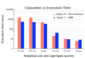
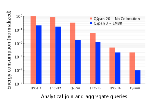
Figure 5: Experiments on a TPC-H Benchmark showing effect of co-location on query response times and resource consumption.

We begin with presenting the result of a set of experiments designed to evaluate the effects of query span on query response times and resource consumption, to further bolster our claim that minimizing query span typically leads to reduced resource consumptions. We then present an extensive set of experiments evaluating the effectiveness of our algorithms at minimizing the query span for a collection of synthetic and real workloads.

5.1 Query Span and Resource Consumption

We conducted a set of experiments analyzing the effect of query span on the total amount of resources consumed, and the total energy consumed, under a variety of settings. We performed this experiment on 20 Amazon EC2 medium instances. We use the same two settings and the same set of queries that we used in the experiments presented in Section 1. The first setting is a horizontally partitioned MySQL cluster, where we evaluate two complex analytical join queries (TPC-H1, TPC-H2), and two single-table aggregate queries (TPC-H3, TPC-H4), on a TPC-H dataset. The second setting is a homegrown distributed query processor that sits atop multiple MySQL instances running on a cluster where predicate evaluations are pushed on to the individual nodes and data is shipped to a single node for perform the final steps. We evaluate a complex join query (Q-Join) and a single-table aggregate query (Q-Sum) on that setup.

To compare the cost of our best co-location scheme LMBR, we run around 10000 additional queries with TPC-H1, TPC-H2, TPC-H3, TPC-H4 , Q-join and Q-Sum on our setup, so that we can construct the hypergraph of these queries. We then perform min-cut partitioning over this hypergraph to get a 20-way partitioning, and then we apply LMBR on this setup. Based on placement given by LMBR, we place the data items across the 20 machines. Then we execute our test queries and carefully make sure that each query is executed on the set of machines that it spans. Query span is calculated by using set-cover algorithm on the placement suggested by LMBR. Average span over these test queries was 3, i.e., data needed for these queries were located on an average of 3 machines using LMBR.

In Figure 5, we plot the query response times of our test queries on the horizontal partitioning placement on 20 machines and we compare it with the query response times when executed on LMBR-suggested placement. We notice that query response times for complex analytical test queries TPC-H1, TPC-H2 and Q-join decrease significantly when executed on LMBR suggested placement. This is because of minimization of overheads caused by distributed analytical processing, e.g., communication overheads in processing complex joins. On the other hand, query response times for test queries TPC-H3, TPC-H4 and Q-Sum increase with co-location. This confirms our intuition that parallelism is more effective for simple queries than for complex queries.

Figure 5 shows that, irrespective of the type of the query, energy consumption decreases significantly with co-location of accessed data items. It shows that most reduction in energy consumption for complex analytical query is for TPC-H1that is almost $79\%$, whereas for Q-Join we observe $31\%$ reduction. For simple aggregate queries, firstly we observe that there can be a tradeoff between query response time and energy consumption on co-location. Secondly, for queries TPC-H3, TPC-H4 where reduction in energy consumption is $77\%$ and $57\%$ and for Q-Sum we observe $71\%$. Depending upon the optimization goal such as query response time or energy minimization or both, one may choose to colocate the data items or not. In this work, we specifically focus at opportunities where co-location is applicable and provides us significant benefits in terms of minimization of energy consumed per query, it may also minimize query response times, for example: in case of complex analytical queries.

This experiment highlights the fact that, query response time may increase or decrease with co-location depending up on the nature of the query (complex analytical or simple aggregate). But in all cases, energy costs reduces with a good data co-location, for example: co-location provided by LMBR.

5.2 Query Span Experiments

We evaluate effectiveness of our proposed algorithms by building a trace-driven simulator to experiment with different data placement policies. The simulator instantiates a number of partitions as needed by the experimental setup, uses a data placement algorithm for distributing the data among the partitions, and replays a query trace against it to measure the query span profiles.

We conducted an extensive experimental study to evaluate our algorithms, using several real and synthetic datasets. Specifically, we used the following three datasets:

• Random: Instead of generating a query workload completely randomly, we use a different approach to better understand the structure of the problem. We first generate a random data item graph of a specified density (edges to nodes ratio). We then randomly generate queries such that the data items in the query form a connected subgraph in the data item graph. For low density data item graphs, this induces significant structure in the query workload that good data placement algorithms can exploit for better performance.

• Snowflake: This is a special case of the above where the data item graph is a tree. This workload attempts to mimic a standard SQL query workload. We treat each column of each relation as a separate data item. An SQL query over such a schema that does not contain a Cartesian product corresponds to a connected subgraph in this graph.

• ISPD98 Benchmark Data Sets: In addition to the above synthetic datasets, we tested our algorithms on standard ISPD98 benchmarks [5]. ISPD98 circuit benchmark suite contains 18 circuits ranging from 12,752 to about 210,000 nodes. Hypergraph density (hyperedges to nodes ratio) in all the ISPD98 circuit benchmarks is close to 1, i.e., these graphs are quite sparse. We show results for the first 10 circuit datasets, that contain 12,752 to 69,429 nodes.

We compare the performance of six algorithms: (1) Random, where the data is replicated and distributed randomly, (2) HPA, the baseline hypergraph partitioning algorithm, (3-6) the four algorithms that we propose, IHPA, PRA, DS, and LMBR (Section 4). We use the hMETIS hypergraph partitioning algorithm [23, 2] as our HPA algorithm. The experiments were run on a Intel Core2 Duo CPU 2.10GHz, 4GB RAM, Windows PC running Windows 7. All plotted numbers (except the numbers for the ISPD98 benchmark) are averages over 10 random runs. For reproducibility, we list the values of the remaining hMETIS parameters: Nruns = 20, CType = 2, RType = 1, VCycle = 1, Reconst = 1, dbglvl = 0.

The key parameters of the dataset that we vary are: (1) $|$D$|$, the number of data items, (2-3) minQuerySize and maxQuerySize, the bounds on the query sizes that are generated, (4) NQ, the number of queries, (5) C, the partition capacity, (6) numPartitions (NPar), the number of partitions, and (7) density of the data item graph (defined to be the ratio of the number of edges to the number of nodes). The default values were: $|$D$|$ = 1000, minQuerySize = 3, maxQuerySize = 11, NQ = 4000, C = 50, NPar = 40, and density = 20.

Figure 6: $(a)-(e)$ Results of the experiments on the Random dataset with homogeneous data items illustrate the benefits of intelligent data placement with replication; the LMBR algorithm produces the best data placement in almost all scenarios. Note that, for clarity, the $y$-axes for several of the graphs do not start at 0. $(f)-(h)$ 3-way replication results with replication factor of each node $RF=3$.

In several of the plots, we also show the average number of data items per query, denoted ADI.

5.2.1 Random Dataset

We begin with showing the results for the Random dataset with homogeneous data items.

Increasing Number of Partitions ($ND$): First, we run experiments with increasing the number of partitions. With the default parameters, a minimum of 20 partitions are needed to store the data items. We increase the number of partitions from 20 to 45, and compute the average query spans, and average execution times, for the six algorithms over 10 runs. Figures 6, and 6 show the results of the experiment. HPA does not do replication, and hence the corresponding plot is a straight line. The performance of the rest of the algorithms, including Random, improves as we allow for replication. Among those, LMBR performs the best, with IHPA a close second. We saw this behavior consistently across almost all of our experiments (including the other datasets). LMBR’s performance does come with a significantly higher execution times as shown in Figure 6. This is because LMBR tends to do a lot of small moves, whereas the other algorithms tend to have a small number of steps (e.g., DS runs the densest subgraph algorithm a fixed number of times, whereas PRA only has three phases). Since data placement is a one-time offline operation, the high execution time of LMBR may be inconsequential compared to the reduction in query span it guarantees.

Increasing Query Size ($ADI$): Second, we vary the number of data items per query from 2 to 10 (by setting minQuerySize = maxQuerySize), choosing the default values for the other parameters. As expected (Figure 6), the average span increase rapidly as the query size increases. The relative performance of the different algorithms is largely unchanged, with LMBR and IHPA performing the best.

Increasing Number of Queries ($NQ$): Next, we vary the number of queries from 1,000 to 11,000, thus increasing the density of the hypergraph (Figure 6). The average query span increases rapidly in the beginning and much more slowly beyond 5,000 queries. Once again the LMBR algorithm finds the best solution by a significant margin compared to the other algorithms.

Increasing Data Item Graph Density: Finally, we vary the data item graph density while from 2 (very sparse) to 20 (dense). The number of partitions was set to 40. As we can see in Figure 6, for low density graphs, the average span of the queries is quite low, and it increases rapidly as the density increases. Note that the average query size did not change, so the performance gap is entirely because of the structure of the query hypergraph for low density data item graphs. Further, we note that the curves flatten out as the density increases, and don’t change significantly beyond 10, indicating that the query workload essentially looks random to the algorithms beyond that point.

Overall, our experimental study indicates that LMBR, despite its high running time, should be the data placement algorithm used for minimizing query span/multi-site overheads and energy consumption in such scenarios (where we do not have any constraints on the number of replicas that must or can be created).

5.2.2 3-Way Replication

Figures 6, 6 and 6 show a set of experimental results comparing the 3-way replication algorithms that we have discussed in Section 4.6.

Increasing Number of Queries ($NQ$): Increasing the number of queries, thus increasing the density of the graph, we observe that PRA based 3-way replication algorithm performs the best. This is in comparison with HPA (no replication), Random 3-way replication and simple distribution algorithm (SDA). As the number of hyperedges increases in the graph average number of hyperedges incident per node also increases. This effects the SDA algorithm, because SDA tries to distribute the 3 copies of the node randomly to the number of hyperedges incident on it. So as average number of incident hyperedges per node increases, it is more likely for SDA to make bad decisions about distribution of replicas among incident hyperedges, hence SDA’s average span increases with number of queries. On the other hand, PRA employs hitting set technique to do a more smarter replica distribution among the incident hyperedges. Increase in number of queries doesn’t seem to effect the query span for PRA, which indicates the effectiveness of PRA approach. Hence, PRA based technique performs consistently better than SDA in this experiment.

Increasing Query Size ($ADI$): Query span for all the algorithms increases with an increase in average data items per query. As we saw that density of the hypergraph affects PRA and SDA, where increase in density doesn’t affect PRA. In this experiment increase in hyperedge size doesn’t affect the density of the hypergraph. Hence query span increases for SDA and PRA. PRA again performs consistently better than other algorithms.

Increasing Data Item Graph Density: PRA again performs the best compared to Random and SDA when density of the graph is varied. Analysis is similar to what we have discussed before in Section 5.2.1.

We do not compare with LMBR for this scenario due to its high running time, and because it cannot guarantee the replication constraint of 3-way replication.

5.2.3 Snowflake Dataset

Figures 7 and 7 show a set of experimental results for the Snowflake dataset. Each of the plotted numbers corresponds to an average over 10 random query workloads. The data item graph itself was generated with the following parameters: the number of levels in the graph was 3, the degree of each relation (the maximum number of tables it may join with) is set to 5, and the number of attributes per table is set to 15. The total number of data items was 2000, requiring a minimum of 20 partitions to store them. Note that we assume homogeneous data items in this case. We plot the average query spans, and the average execution times as the number of partitions increases from 20 to 45.

We also conducted a similar set of experiments with heterogeneous data item sizes, where we generated TPC-H style queries with data item sizes adhering to the TPC-H benchmark. We chose the scale factor of 25, which means the highest data item size is 28GB and smallest data item size is 25KB. This results in a high skew among the table column sizes. Data item size is calculated as $Size(columnDatatype)*noRows$. The partition capacity was fixed at 100GB, and we once again plot the average query spans and the average execution times as the number of partitions increases from 20 to 45. The results are shown in Figures 8 and 8.

Our results here corroborate the results on the Random dataset. We once again see that LMBR performs the best, finding significantly better data layouts than the other algorithms. The performance differences are quite drastic with homogeneous data item sizes – with 45 partitions, LMBR is able to achieve an average query span of just 1.5, whereas the baseline HPA results in an average span of 3.5. However, we observe that with heterogeneous data item sizes, the advantages of using smart data placement algorithms are lower. With an extreme skew among the data item sizes, the replication and data placement choices are very limited.

Figure 7: Results of the Experiments on the Snowflake Dataset

5.2.4 ISPD98 Benchmark Dataset

Finally, Figure 9 shows the comparative results for first ten of hypergraphs from the ISPD98 Benchmark Suite, commonly used in the hypergraph partitioning literature. The number of hyperedges in the datasets range from 14111 to 75196 and number of nodes range from 12752 to 69429. Here we set the partition capacity so that exactly 20 partitions are sufficient to store the data items, and we plot the results with number of partitions set to 35. The hypergraphs in this dataset tend to have fairly low densities, resulting in low query spans. In fact, LMBR is able to achieve an average query span of close to the minimum possible (i.e., 1) with 35 partitions. Most of the other algorithms perform about 20 to 40% worse compared to LMBR.

Figure 8: Results of the Experiments on a TPC-H style Benchmark with unequal data item sizes. The relation sizes were calculated assuming a scale factor of 25.

Figure 9: Results of the experiments on the first 10 hypergraphs, ibm01, …, ibm10, from the ISPD98 Benchmark Dataset

These additional experiments further corroborate our claim that intelligent data placement with replication can significantly reduce the coordination overheads in data centers, and further that our LMBR algorithm outperforms rest of the algorithms significantly.

6 Conclusions

In this paper, we solve the combined problem of data placement and replication, given a query workload, to minimize the total resource consumption and by proxy, the total energy consumption, in very large distributed or multi-site read-only data stores. Directly optimizing for either of these metrics is likely infeasible in most practical scenarios because of the large number of factors involved. We instead identify query span, the number of machines involved in executing a query, as having a direct and significant impact on the total resource consumption, and focus on minimizing the average query span for a given query workload. We formulated and analyzed the problems of data placement and replica selection for this metric, and drew connections to several well-studied graph theoretic concepts. We used these connections to develop a series of algorithms to solve this problem, and our extensive experimental evaluation over several datasets demonstrated that our algorithms can result in drastic reductions in average query spans. We are planning to extend our work in several different directions. As we discussed earlier, we believe that temporal scheduling algorithms can be used to correct the load imbalance that may result from optimizing for query span alone; although analysis tasks are usually not latency sensitive, there are still often deadlines that need to be satisfied. We plan to study how to incorporate such deadlines into our framework. We are also planning to study how to efficiently track changes in the query workload nature online, and how to adapt the replication decisions online.

References

- [1] http://www.cs.umd.edu/~ashwin/fullpaper.pdf.
- [2] hMETIS: A hypergraph partitioning package, http://glaros.dtc.umn.edu/gkhome/metis/hmetis/overview.
- [3] MLPart, http://vlsicad.ucsd.edu/gsrc/bookshelf/slots/partitioning/mlpart/.
- [4] N. Alon, P. D. Seymour, and R. Thomas. A separator theorem for graphs with an excluded minor and its applications. In STOC, 1990.
- [5] C. J. Alpert. The ISPD98 circuit benchmark suite. In Proc. of Intl. Symposium on Physical Design, 1998.
- [6] H. Amur, J. Cipar, V. Gupta, G. Ganger, M. Kozuch, and K. Schwan. Robust and flexible power-proportional storage. In SoCC, 2010.
- [7] Y. Asahiro, K. Iwama, H. Tamaki, and T. Tokuyama. Greedily finding a dense subgraph. In SWAT, 1996.
- [8] R. B. Boppana. Eigenvalues and graph bisection: An average-case analysis. In FOCS, 1987.
- [9] A. E. Caldwell, A. B. Kahng, and I. L. Markov. Design and implementation of move-based heuristics for VLSI hypergraph partitioning. J. Exp. Algorithmics, 5:5, 2000.
- [10] M. Chowdhury, M. Zaharia, J. Ma, M. I. Jordan, and I. Stoica. Managing data transfers in computer clusters with Orchestra. In SIGCOMM, pages 98–109, 2011.
- [11] D. Colarelli and D. Grunwald. Massive arrays of idle disks for storage archives. In Supercomputing, 2002.
- [12] C. Curino, Y. Zhang, E. P. C. Jones, and S. Madden. Schism: a workload-driven approach to database replication and partitioning. PVLDB, 3(1):48–57, 2010.
- [13] J. Dittrich, J.-A. Quiané-Ruiz, A. Jindal, Y. Kargin, V. Setty, and J. Schad. Hadoop++: making a yellow elephant run like a cheetah (without it even noticing). PVLDB, 3:515–529, September 2010.
- [14] Z. Du, J. Hu, Y. Chen, Z. Cheng, and X. Wang. Optimized qos-aware replica placement heuristics and applications in astronomy data grid. Journal of Systems and Software, 84(7):1224 – 1232, 2011.
- [15] D. Economou, S. Rivoire, and C. Kozyrakis. Full-system power analysis and modeling for server environments. In In Workshop on Modeling Benchmarking and Simulation (MOBS), 2006.
- [16] M. Y. Eltabakh, Y. Tian, F. Özcan, R. Gemulla, A. Krettek, and J. McPherson. Cohadoop: Flexible data placement and its exploitation in hadoop. PVLDB, 4(9):575–585, 2011.
- [17] U. Feige, G. Kortsarz, and D. Peleg. The dense k-subgraph problem. Algorithmica, 1999.
- [18] H. Ferhatosmanoglu, A. S. Tosun, and A. Ramachandran. Replicated declustering of spatial data. In PODS, 2004.
- [19] M. Garey and D. Johnson. “Computers and Intractability: A Guide to the Theory of NP-Completeness”. 1979.
- [20] G. Graefe. Database servers tailored to improve energy efficiency. In Proceedings of EDBT workshop on Software engineering for tailor-made data management, 2008.
- [21] S. Harizopoulos, M. A. Shah, J. Meza, and P. Ranganathan. Energy efficiency: The new holy grail of data management systems research. In CIDR, 2009.
- [22] L.-Y. Ho, J.-J. Wu, and P. Liu. Optimal algorithms for cross-rack communication optimization in mapreduce framework. In IEEE International Conference on Cloud Computing, 2011.
- [23] G. Karypis, R. Aggarwal, V. Kumar, and S. Shekhar. Multilevel hypergraph partitioning: Application in VLSI domain. In IEEE VLSI, pages 69–529, 1999.
- [24] G. Karypis and V. Kumar. Multilevel k-way hypergraph partitioning. In Proc. of DAC, pages 343–348, 1998.
- [25] M. Koyutürk and C. Aykanat. Iterative-improvement-based declustering heuristics for multi-disk databases. Information Systems, 2005.
- [26] W. Lang and J. M. Patel. Towards eco-friendly database management systems. In CIDR, 2009.
- [27] W. Lang and J. M. Patel. Energy management for mapreduce clusters. PVLDB, 3(1):129–139, 2010.
- [28] J. Leverich and C. Kozyrakis. On the energy (in)efficiency of hadoop clusters. HotPower, 2009.
- [29] D.-R. Liu and S. Shekhar. Partitioning similarity graphs: A framework for declustering problems. Information Systems, 1996.
- [30] H. Meyerhenke, B. Monien, and T. Sauerwald. A new diffusion-based multilevel algorithm for computing graph partitions. J. Parallel Distrib. Comput., 69(9), 2009.
- [31] J. Mondal and A. Deshpande. Managing large dynamic graphs efficiently. In SIGMOD, 2012.
- [32] T. A. Neves, L. M. de A. Drummond, L. S. Ochi, C. Albuquerque, and E. Uchoa. Solving replica placement and request distribution in content distribution networks. Electronic Notes in Discrete Mathematics, 36:89–96, 2010.
- [33] K. Y. Oktay, A. Turk, and C. Aykanat. Selective replicated declustering for arbitrary queries. In Euro-Par, 2009.
- [34] C. Olston, B. Reed, U. Srivastava, R. Kumar, and A. Tomkins. Pig latin: a not-so-foreign language for data processing. In SIGMOD, 2008.
- [35] A. Pavlo, E. Paulson, A. Rasin, D. J. Abadi, D. J. DeWitt, S. Madden, and M. Stonebraker. A comparison of approaches to large-scale data analysis. In SIGMOD, 2009.
- [36] E. Pinheiro and R. Bianchini. Energy conservation techniques for disk array-based servers. In Supercomputing, 2004.
- [37] A. Quamar, K. A. Kumar, and A. Deshpande. Sword: Scalable workload-aware data placement for transactional workloads. In In submission.
- [38] H. D. Simon and S.-H. Teng. How good is recursive bisection? SIAM J. Sci. Comput., 18(5):1436–1445, 1997.
- [39] D. Thain and M. Livny. Building reliable clients and servers. In I. Foster and C. Kesselman, editors, The Grid: Blueprint for a New Computing Infrastructure. Morgan Kaufmann, 2003.
- [40] A. Thusoo, J. S. Sarma, N. Jain, Z. Shao, P. Chakka, S. Anthony, H. Liu, P. Wyckoff, and R. Murthy. Hive: a warehousing solution over a map-reduce framework. PVLDB, 2:1626–1629, August 2009.
- [41] A. A. Tosun and H. Ferhatosmanoglu. Optimal parallel I/O using replication. In ICPP, 1997.
- [42] A. S. Tosun. Replicated declustering for arbitrary queries. In ACM symposium on Applied computing, 2004.
- [43] D. Tsirogiannis, S. Harizopoulos, and M. A. Shah. Analyzing the energy efficiency of a database server. In SIGMOD, 2010.
- [44] T. White. Hadoop: The Definitive Guide. O’Reilly Media, 1st edition, June 2009.
- [45] O. Wolfson, S. Jajodia, and Y. Huang. An adaptive data replication algorithm. ACM TODS, 22:255–314, 1997.
- [46] O. Wolfson and A. Milo. The multicast policy and its relationship to replicated data placement. ACM TODS, 16:181–205, March 1991.