Renormalization group approach to Einstein-Rosen waves

Abstract

We present a renormalization group analysis to Einstein-Rosen waves or vacuum spacetimes with whole-cylinder symmetry. It is found that self-similar solutions appear as fixed points in the renormalization group transformation. These solutions correspond to the explosive gravitational waves and the collapsing gravitational waves at late times and early times, respectively. Based on the linear perturbation analysis of the self-similar solutions, we conclude that the self-similar evolution is stable as explosive gravitational waves under the condition of no incoming waves, while it is weakly unstable as collapsing gravitational waves. The result implies that self-similar solutions can describe the asymptotic behavior of more general solutions for exploding gravitational waves and thus extends the similarity hypothesis in general relativity from spherical symmetry to cylindrical symmetry.

I Introduction

Renormalization group analysis is a powerful tool for obtaining asymptotic behavior of solutions of partial differential equations Bricmont:1994 . Koike et al. Koike:1995jm ; Koike:1999eg have applied this method to a self-gravitating system in general relativity and successfully explained critical behavior together with the critical exponent in gravitational collapse. Ibáñez and Jhingan Ibanez:2004pt ; Ibanez:2007yq have applied this method to inhomogeneous cosmology and analyzed the stability of scale-invariant asymptotic states (see also Refs. Chen:1994zza ; Chen:1995ena ; Iguchi:1997mx ).

Fixed points under renormalization group transformation are very important for the asymptotic analysis. The fixed-point solutions in general relativity generally correspond to self-similar solutions, which are defined as spacetimes that admit a homothetic Killing vector. Self-similar solutions arise from the scale-invariance of general relativity. Carr Carr:1993 ; Carr:2005uf has conjectured that under certain physical circumstances, spherically symmetric solutions will naturally evolve to a self-similar form from complicated initial conditions, and this is termed as the similarity hypothesis. This conjecture has been strongly supported in the gravitational collapse of a perfect fluid by numerical simulation and linear stability analysis Harada:2001nh .

Although the similarity hypothesis has been proposed originally in spherical symmetry, there is evidence that supports the validity of the conjecture also in cylindrical symmetry. Nakao et al. Nakao:2009jp have numerically simulated the collapse of the dust cylinder and the subsequent emission of gravitational waves in special cylindrical symmetry. Their numerical simulation suggests that gravitational waves gradually approach a self-similar form.

The vacuum Einstein equations in this symmetry can be analytically integrated, and solutions are called the Einstein-Rosen waves Einstein:1937qu . Since this system admits two commutative spatial Killing vectors and still retains the dynamical degrees of freedom corresponding to gravitational waves, it provides us with a good toy model in which we can learn the physical nature of gravitational waves. Harada et al. Harada:2008rx have derived self-similar Einstein-Rosen waves and identified one of them with the attractor solution that Nakao et al. Nakao:2009jp reported. In this paper, we recover the self-similar Einstein-Rosen waves as a fixed point of the renormalization group analysis. Then, we perform the linearized perturbation analysis of these solutions (fixed points) and determine their stability analytically using an eigenvalue analysis.

This paper is organized as follows. In Sec. II, we show the field equations for Einstein-Rosen waves. In Sec. III, we introduce the renormalization group analysis as a scaling transformation and self-similar Einstein-Rosen waves as fixed points. In Sec. IV, we apply linear perturbation theory to the self-similar solutions. In Sec. V, we analyze the behavior of the perturbations at the boundaries. In Sec. VI, we show that the self-similar Einstein-Rosen waves are stable and unstable at late times and at early times, respectively, under appropriate boundary conditions. In Sec. VII, we conclude the paper. We use the units in which $c=1$.

II Einstein-Rosen waves

We consider cylindrically symmetric spacetimes with the azimuthal Killing vector $\partial/\partial\phi$ and the translational Killing vector $\partial/\partial z$. We additionally assume that these two Killing vectors are hypersurface orthogonal for whole-cylinder symmetry. Vacuum spacetimes with whole-cylinder symmetry are called Einstein-Rosen waves Einstein:1937qu . The line element in Einstein-Rosen waves is given by

$$ds^{2}=e^{2(\gamma-\psi)}(-dt^{2}+dx^{2})+e^{-2\psi}x^{2}d\phi^{2}+e^{2\psi}dz^{2}.$$ (1)

The nontrivial Einstein equations take the following form:

$$-\psi_{,tt}+\psi_{,xx}+\frac{1}{x}\psi_{,x}=0,$$ (2)

$$\gamma_{,x}=x(\psi_{,x}^{2}+\psi_{,t}^{2}),$$ (3)

$$\gamma_{,t}=2x\psi_{,x}\psi_{,t}.$$ (4)

We define new variables $h(x,t)$ and $f(x,t)$, which are more convenient to our analysis, by

$$f^{2}=\frac{h^{2}}{x^{2}}e^{2\gamma}\quad\mbox{and}\quad h^{2}=xe^{-2\psi},$$ (5)

respectively. Then, the line element is rewritten in the following form:

$$ds^{2}=f^{2}(-dt^{2}+dx^{2})+x(h^{2}d\phi^{2}+h^{-2}dz^{2}),$$ (6)

where $f$ and $h$ satisfy

$$f_{,t}=\pm 2xf\frac{h_{,x}}{h}\left[{\frac{1}{4x^{2}}+\frac{1}{x}\frac{f_{,x}}{f}-\frac{h_{,x}^{2}}{h^{2}}}\right]^{1/2},$$ (7)

and

$$h_{,t}=\pm h\left[{\frac{1}{4x^{2}}+\frac{1}{x}\frac{f_{,x}}{f}-\frac{h_{,x}^{2}}{h^{2}}}\right]^{1/2},$$ (8)

respectively, where (and hereafter), in the case of double sign, we should uniformly choose either an upper sign or lower sign. The wave equation (2) is identically satisfied from the above two equations. Hence, we have the desired evolution equations for the metric functions in a form suitable for a renormalization group analysis.

III Renormalization group analysis

Since we are interested in the solution in the asymptotic regime, we shall explore now the scale-invariant properties of the system. We consider the following scale transformation and define the scaled functions, $h_{(L)}(x,t)$ and $f_{(L)}(x,t),$ as follows:

$$x \to Lx,$$ (9)

$$t \to L^{\alpha}t,$$ (10)

$$h \to L^{a}h(Lx,L^{\alpha}t)=h_{(L)}(x,t),$$ (11)

$$f \to L^{b}f(Lx,L^{\alpha}t)=f_{(L)}(x,t).$$ (12)

Here, $L$ is the scaling parameter, and scaled quantities $h_{(L)}$ and $f_{(L)}$ satisfy the same evolution equations, i.e., Eqs. (7) and (8). From the structure of dynamical system, it is easy to see that $t$ scales in the same way as $x$, fixing $\alpha=1$. There is no further constraint on scaling exponents $a$ and $b$. Putting $t=1$ and redefining, in succession, $Lx$ by $x$ and $L$ by $t$, in Eqs. (11) and (12), we find

$$h(x,t) = t^{-a}h_{(L)}(x/t,1),$$ (13)

$$f(x,t) = t^{-b}f_{(L)}(x/t,1)$$ (14)

in the scaling regime. Note that the quantities $h_{(L)}(x/t,1)$ and $f_{(L)}(x/t,1)$ are evaluated at some initial time ($t=1$ here) and are determined as fixed points of the renormalization group equations as illustrated below.

In what follows, we adopt the mechanism developed by Bricmont et al. Bricmont:1994 . Defining $L=\exp(\tau)$, we can rewrite the scaling behavior of Eqs. (11) and (12) into a set of coupled ordinary differential equations:

$$\frac{dh_{(L)}}{d\tau} = \left.ah_{(L)}+xh_{(L),x}+h_{(L),t}\right|_{t=1},$$ (15)

$$\frac{df_{(L)}}{d\tau} = \left.bf_{(L)}+xf_{(L),x}+f_{(L),t}\right|_{t=1},$$ (16)

where the quantities on the right-hand side are evaluated at initial time and are functions only of $x$. The fixed-point solutions $h_{(L)}^{*}$ and $f_{(L)}^{*}$ are defined by

$$\frac{dh_{(L)}^{*}}{d\tau}=0,\quad\frac{df_{(L)}^{*}}{d\tau}=0.$$ (17)

Therefore, we have fixed fixed points as solutions of a set of coupled nonlinear ordinary differential equations:

$$ah_{(L)}+xh_{(L),x}+h_{(L)}\Psi=0,$$ (18)

$$bf_{(L)}+xf_{(L),x}+2xf_{(L)}\frac{h_{(L),x}}{h_{(L)}}\Psi=0,$$ (19)

where $\Psi$ is defined as

$$\Psi=\pm\left[\frac{1}{4x^{2}}+\frac{1}{x}\frac{f_{(L),x}}{f_{(L)}}-\left(\frac{h_{(L),x}}{h_{(L)}}\right)^{2}\right]^{1/2}.$$ (20)

Here and henceforth, we have dropped superscript * from $h_{(L)}$ and $f_{(L)}$ for brevity. These equations decouple on recombination, and we have the following master equation for $h_{(L)}$:

$$\frac{h_{(L),x}}{h_{(L)}}=-\frac{a}{x}\pm\left[\frac{a^{2}+b-1/4}{x^{2}(1-x^{2})}\right]^{1/2}.$$ (21)

The other metric function $f_{(L)}$ can now be recovered as a solution to an ordinary differential equation:

$$\frac{f_{(L),x}}{f_{(L)}}=-\frac{b}{x}+\frac{2(a^{2}+b-1/4)}{x(1-x^{2})}\mp\frac{2a\sqrt{a^{2}+b-1/4}}{x\sqrt{1-x^{2}}}.$$ (22)

We are interested in the domain $0<x<1$, which now corresponds to the spacetime inside the light cone $0<x<t$. This restricts the parameter space to $a^{2}+b-1/4>0$. Equations (21) and (22) can be easily integrated to give the fixed points

$$h_{(L)} = x^{-a\mp\Delta}(1-\sqrt{1-x^{2}})^{\pm\Delta},$$ (23)

$$f_{(L)} = c_{f}x^{-b+2\Delta^{2}\pm 2a\Delta}(1-x^{2})^{-\Delta^{2}}(1-\sqrt{1-x^{2}})^{\mp 2a\Delta},$$ (24)

where $c_{f}$ is a constant of integration and $\Delta=a^{2}+b-1/4$. Recovering time dependence through Eqs. (13) and (14), we obtain

$$h(x,t) = x^{-a\mp\Delta}(t-\sqrt{t^{2}-x^{2}})^{\pm\Delta},$$ (25)

$$f(x,t) = c_{f}x^{-b+2\Delta^{2}\pm 2a\Delta}(t^{2}-x^{2})^{-\Delta^{2}}(t-\sqrt{t^{2}-x^{2}})^{\mp 2a\Delta}.$$ (26)

The light cone splits the spacetime domain $t>0$ into two parts, and we have another solution corresponding to the region $x>t>0$ and $\Delta<0$. In fact, Fig. 1 shows that the light cone splits the spacetime into four parts if we consider both $t>0$ and $t<0$. For the moment, we focus on domain I and later on IV, i.e., the interior of the light cone. For domains II and III, i.e., the exterior of the light cone, we have another solution corresponding to $x>|t|>0$ and $\Delta<0$, which is out of the scope of the present paper.

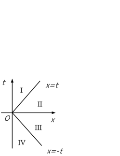
Figure 1: The light cone splits the spacetime into four parts. In the current paper, we focus on domains I and IV, i.e., the interior of the light cone.

These solutions coincide with the self-similar or homothetic solutions derived in Ref. Harada:2008rx , in which the solutions are further restricted by imposing the solution to be either with a regular axis or a conically singular axis. Then, the solutions are parametrized by two parameters $\kappa$ and $\lambda$. The parameter $\kappa$ plays a more important role since it determines the physical nature of the spacetime, while $\lambda$ just controls the deficit angle of the axis. The correspondence between $a$, $b$, and $c_{f}$ in the above obtained expression and $\kappa$ and $\lambda$ in the expression given in Ref. Harada:2008rx is the following:

$$\pm\Delta=\kappa,\quad a=\kappa-1/2,\quad b=\kappa,\quad c_{f}^{2}=2^{-4\kappa^{2}}e^{2\lambda},$$ (27)

where we should note that $\Delta\geq 0$. Note that we have started the analysis in the domain $0<x<t$. Here, it should also be noted that both $\kappa=0$ and $1/2$ correspond to the flat spacetime, and $\kappa=-1/2$ corresponds to the Kasner solution with exponents $(-1/2,2/3,2/3)$ or the locally rotationally symmetric Kasner solution. The $x=t$ surface is a null singularity for $0<\kappa^{2}<1/4$ and $1/4<\kappa^{2}<3/8$, a regular surface admitting an extension beyond it for $3/8<\kappa^{2}<1/2$, and a null infinity for $\kappa^{2}\geq 1/2$. We can further divide the case of $3/8<\kappa^{2}<1/2$ into the case of $\kappa^{2}=1/2-1/(4n)$ ($n=2,3,\cdots$) and otherwise. In the former, the $x=t$ surface admits an analytic extension beyond it, while in the latter, this surface only admits a finitely differentiable extension. In general, these solutions describe exploding gravitational waves. If we flip the sign of $t$, these solutions describe the collapse of gravitational waves. The fully detailed description of the physical nature and causal structure of these solutions is given in Ref. Harada:2008rx . The parameter value which fits the result of the numerical simulation by Nakao et al. Nakao:2009jp is $\kappa=-0.0206$, for which the surface $x=t$ corresponds to a null singularity, which is physically a shock of gravitational waves, and the spacetime cannot be extended beyond it.

IV Linear perturbation analysis

We introduce the perturbation of the fixed point solution as follows:

$$h_{(L)} = h_{(L)}^{*}(1+\delta h_{(L)}),$$ (28)

$$f_{(L)} = f_{(L)}^{*}(1+\delta f_{(L)}).$$ (29)

Assuming $|\delta h_{(L)}|\ll 1$ and $|\delta f_{(L)}|\ll 1$, we linearize the field equations for the perturbation. The linearized perturbed equations take the form

$$\frac{d\delta h}{d\tau} = \left(x-\frac{1}{\Psi}\frac{h^{*}_{,x}}{h^{*}}\right)\delta h_{,x}+\frac{1}{2x\Psi}\delta f_{,x},$$ (30)

$$\frac{d\delta f}{d\tau} = 2x\left[\Psi-\frac{1}{\Psi}\left(\frac{h^{*}_{,x}}{h^{*}}\right)^{2}\right]\delta h_{,x}+\left(x+\frac{1}{\Psi}\frac{h^{*}_{,x}}{h^{*}}\right)\delta f_{,x},$$ (31)

where we have dropped the subscript $(L)$ from the metric functions for brevity. Note that all the quantities are evaluated at the fixed points (emphasized by an * ) and, hence, are known functions of $x$ given by Eqs. (23) and (24).

We now compute the normal modes with the dependence $\delta h=e^{\omega\tau}\rho(x)$ and $\delta f=e^{\omega\tau}\sigma(x)$, where $\omega$ is a constant. From Eqs. (30) and (31), we obtain

$$\omega\rho = \left(x+\frac{1}{x}+\frac{a}{x\Psi}\right)\rho_{,x}+\frac{1}{2x\Psi}\sigma_{,x},$$ (32)

$$\omega\sigma = \left[2\left(x\Psi-\frac{1}{x}\Psi-\frac{a^{2}}{x\Psi}\right)-\frac{4a}{x}\right]\rho_{,x}+\left(x-\frac{1}{x}-\frac{a}{x\Psi}\right)\sigma_{,x}.$$ (33)

Combining the two equations, we can solve for $\sigma$ as

$$\omega\sigma=-2\omega(a\mp\Delta\sqrt{1-x^{2}})\rho\mp 2\Delta x\sqrt{1-x^{2}}\rho_{,x}.$$ (34)

We can recover a master equation for $\rho(x)$ from Eqs. (32), (33) and (34), i.e.,

$$\rho_{,xx}+\frac{2(\omega-1)x^{2}+1}{x(1-x^{2})}\rho_{,x}-\frac{\omega(\omega-1)}{1-x^{2}}\rho=0.$$ (35)

Again, the above is estimated at $t=1$, and, hence, $x$ should be regarded as $x/t$ in the notation of Harada et al. Harada:2008rx . Note that there is no a priori reason to assume that $\omega$ is real.

We define $\zeta=1/\sqrt{1-x^{2}}$ and $g=\zeta^{\omega}\rho$. Then, Eq. (35) transforms to

$$\frac{d}{d\zeta}\left[(1-\zeta^{2})\frac{dg}{d\zeta}\right]+\omega(\omega+1)g=0,$$ (36)

where $0<x<1$ corresponds to $\zeta>1$. This is the Legendre differential equation. Note that this equation has symmetry for the replacement of the parameter $\omega\leftrightarrow-(\omega+1)$. The Legendre functions of the first and second kinds—$P_{\omega}(\zeta)$ and $Q_{\omega}(\zeta)$, respectively—are solutions of the Legendre differential equation. General solutions can be expressed in terms of the Legendre functions simply as

$$\rho=(1-x^{2})^{\omega/2}\left[c_{1}P_{\omega}\left(\frac{1}{\sqrt{1-x^{2}}}\right)+c_{2}Q_{\omega}\left(\frac{1}{\sqrt{1-x^{2}}}\right)\right].$$ (37)

The above expression is convenient for ${\rm Re}(\omega)\geq-1/2$. For ${\rm Re}(\omega)<-1/2$, due to the symmetry of the Legendre differential equation, we can express the solutions in terms of the Legendre functions with indices $\nu=-(\omega+1)$ in the range ${\rm Re}(\nu)>-1/2$. Then, we find the following expression that is more convenient:

$$\rho=(1-x^{2})^{\omega/2}\left[\bar{c}_{1}P_{-(\omega+1)}\left(\frac{1}{\sqrt{1-x^{2}}}\right)+\bar{c}_{2}Q_{-(\omega+1)}\left(\frac{1}{\sqrt{1-x^{2}}}\right)\right].$$ (38)

The solution for another perturbation $\sigma$ of the metric functions can be constructed by Eq. (34).

V Behavior of the linear perturbations

We impose the boundary conditions from the physical requirements and study the allowed range of $\omega$. To do this, we need the asymptotic behavior of $P_{\nu}(z)$ and $Q_{\nu}(z),$ for $\mbox{Re}(\nu)\geq-1/2$ at $z=1$ and $z=\infty$, which are given in Refs. Erdelyi:1953 ; Virchenko:2001 ; Oldham:2008 . The asymptotic behavior of $P_{\nu}(z)$ and $Q_{\nu}(z)$ at $z=1$ are given by

$$P_{\nu}(1)=1,$$ (39)

and

$$Q_{\nu}(z)\simeq-\frac{1}{2}\ln\frac{z-1}{2}-\gamma-\psi(\nu+1),\quad(\nu\neq-1,-2,-3,\ldots,),$$ (40)

where $\gamma$ is the Euler number and $\psi(z)=\displaystyle\frac{d}{dz}(\ln\Gamma(z))$ is the polygamma function. The asymptotic behavior of $P_{\nu}(z)$ and $Q_{\nu}(z)$ for $z\to\infty$ is given by

$$P_{\nu}(z) \simeq 2^{\nu}\pi^{-1/2}\Gamma(\nu+1/2)z^{\nu}/\Gamma(1+\nu),~{}({\rm Re}(\nu)>-1/2)$$ (41)

$$P_{-1/2}(z) \simeq \frac{\sqrt{2}}{\pi}\frac{\ln(8z)}{\sqrt{z}},$$ (42)

$$P_{-1/2+ip}(z) \simeq \frac{i(2z)^{-1/2}}{\pi\tanh(\pi p)}\left[\frac{\Gamma(1/2+ip)^{2}}{\Gamma(1+2ip)}(2z)^{-ip}-\frac{\Gamma(1/2-ip)^{2}}{\Gamma(1-2ip)}(2z)^{ip}\right],$$ (43)

where $p\neq 0$, $p\in\mathbb{R}$ and

$$Q_{\nu}(z)\simeq 2^{-\nu-1}\pi^{1/2}\Gamma(\nu+1)z^{-\nu-1}/\Gamma(\nu+3/2),$$ (44)

respectively.

To make the discussion clear, we hereafter concentrate on the stability of self-similar solutions with a regular or only conically singular axis. If we assume $\kappa=0$ for the parametrization of Harada et al. Harada:2008rx , we find all the solutions of the family are flat. Thus, we can assume $\kappa\neq 0$ or $\Delta\neq 0$ without the loss of generality. The asymptotic behavior of the solutions at $x=0$ and $x=1$ are given as follows.

V.1 ${\rm Re}(\omega)>-1/2$ and $\omega\neq 0$

For ${\rm Re}(\omega)>-1/2$, we find

$$\rho \simeq c_{1}+c_{2}[-\ln x+\ln 2-\gamma-\psi(\omega+1)],$$ (45)

$$\sigma \simeq -2c_{1}(a\mp\Delta)+2c_{2}[-(a\mp\Delta)[-\ln x+\ln 2-\gamma-\psi(\omega+1)]\pm\Delta/\omega]$$ (46)

at $x=0$ and

$$\rho \simeq c_{1}2^{\omega}\pi^{-1/2}\frac{\Gamma(\omega+1/2)}{\Gamma(\omega+1)}+c_{2}2^{-\omega-1}\pi^{1/2}\frac{\Gamma(\omega+1)}{\Gamma(\omega+3/2)}(1-x^{2})^{\omega+1/2},$$ (47)

$$\sigma \simeq -2c_{1}a2^{\omega}\pi^{-1/2}\frac{\Gamma(\omega+1/2)}{\Gamma(\omega+1)}\mp 2c_{2}\Delta 2^{-\omega-1}\pi^{1/2}\frac{(\omega+1/2)\Gamma(\omega+1)}{\Gamma(\omega+3/2)}(1-x^{2})^{\omega}$$ (48)

at $x=1$, where (and hereafter) only the relevant terms are shown. Note that the gamma function has no zeroes.

V.2 ${\rm Re}(\omega)<-1/2$

For ${\rm Re}(\omega)<-1/2$, we find

$$\rho \simeq \bar{c}_{1}+\bar{c}_{2}[-\ln x+\ln 2-\gamma-\psi(-\omega)],$$ (49)

$$\sigma \simeq -2\bar{c}_{1}(a\mp\Delta)+2\bar{c}_{2}[-(a\mp\Delta)[-\ln x+\ln 2-\gamma-\psi(-\omega)]\pm\Delta/\omega]$$ (50)

at $x=0$ and

$$\rho \simeq \bar{c}_{1}\frac{2^{-\omega-1}}{\pi^{1/2}}\frac{\Gamma(-\omega-1/2)}{\Gamma(-\omega)}(1-x^{2})^{\omega+1/2}+\bar{c}_{2}2^{\omega+1/2}\pi^{1/2}\frac{\Gamma(-\omega)}{\Gamma(-\omega+1/2)},$$ (51)

$$\sigma \simeq -\bar{c}_{2}a2^{\omega+3/2}\pi^{1/2}\frac{\Gamma(-\omega)}{\Gamma(-\omega+1/2)}\mp\bar{c}_{1}\Delta\frac{2^{-\omega-1/2}}{\pi^{1/2}}\frac{(\omega+1/2)\Gamma(-\omega-1/2)}{\omega\Gamma(-\omega)}(1-x^{2})^{\omega}$$ (52)

at $x=1$.

V.3 $\omega=0$

For $\omega=0$, from Eq. (34), we find $\rho=\mbox{const}$. Substituting this into Eq. (33), we find $\sigma=\mbox{const}$. This corresponds to the rescaling of $t$ and $x$ by $At$ and $Ax$, where $A$ is a positive constant. Hence, this is not a physical mode but a gauge mode. In the following, we exclude this zero mode from the analysis for this reason.

V.4 $\omega=-1/2$

For $\omega=-1/2$, we find

$$\rho \simeq c_{1}+c_{2}[-\ln x+\ln 2-\gamma-\psi(1/2)],$$ (53)

$$\sigma \simeq -2c_{1}(a\mp\Delta)+2c_{2}[-(a\mp\Delta)[-\ln x+\ln 2-\gamma-\psi(1/2)]\mp 2\Delta]$$ (54)

at $x=0$, and

$$\rho \simeq \frac{\sqrt{2}}{\pi}c_{1}\ln\frac{8}{\sqrt{1-x^{2}}}+\frac{\pi}{\sqrt{2}}c_{2},$$ (55)

$$\sigma \simeq -\frac{2\sqrt{2}}{\pi}c_{1}\left(a\ln\frac{8}{\sqrt{1-x^{2}}}\mp\frac{2\Delta}{\sqrt{1-x^{2}}}\right)-\sqrt{2}\pi c_{2}a$$ (56)

at $x=1$.

V.5 $\omega=-1/2+ip$ ($p\neq 0$ and $p\in\mathbb{R}$)

For $\omega=-1/2+ip$, we find

$$\rho \simeq c_{1}+c_{2}[-\ln x+\ln 2-\gamma-\psi(1/2+ip)],$$ (57)

$$\sigma \simeq -2c_{1}(a\mp\Delta)+2c_{2}[-(a\mp\Delta)[-\ln x+\ln 2-\gamma-\psi(1/2+ip)]\mp 2\Delta]$$ (58)

at $x=0$, and

$$\rho \simeq c_{1}i\frac{2^{-1/2+ip}}{\pi\tanh(\pi p)}\left[\frac{\Gamma(1/2+ip)^{2}}{\Gamma(1+2ip)}2^{-2ip}(1-x^{2})^{ip}-\frac{\Gamma(1/2-ip)^{2}}{\Gamma(1-2ip)}\right]$$ (59)

$$+c_{2}2^{-1/2-ip}\pi^{1/2}\frac{\Gamma(1/2+ip)}{\Gamma(1+ip)}(1-x^{2})^{ip},$$

$$\sigma \simeq -\frac{2^{3/2-ip}}{-1/2+ip}\Delta\left[\frac{c_{1}}{\pi\tanh(\pi p)}\frac{\Gamma(1/2+ip)^{2}}{\Gamma(1+2ip)}+c_{2}\pi^{1/2}\frac{\Gamma(1/2+ip)}{\Gamma(1+ip)}\right](1-x^{2})^{-1/2+ip}$$ (60)

at $x=1$.

VI Normal modes and stability analysis

To see the stability in terms of normal modes, we impose boundary conditions at $x=0$ and $x=1$ and see whether a growing mode exits or not. It is not trivial what boundary conditions we should impose on the solution. At least, the perturbation must be regular at both points; otherwise the linear perturbation scheme should break down. Noting $a\mp\Delta=-1/2$, the regularity at $x=0$ requires $c_{2}=0$ for ${\rm Re}(\omega)\geq-1/2$ and $\bar{c}_{2}=0$ for ${\rm Re}(\omega)<-1/2$ because of the logarithmic divergence of the Legendre function of the second kind at $x=0$. We additionally impose regularity at $x=1$ and then find that only ${\rm Re}(\omega)>-1/2$ is allowed. Conversely, for ${\rm Re}(\omega)>-1/2$ and $c_{2}=0$, the normal modes are regular and analytic both at $x=0$ and $x=1$.

VI.1 Stability of the late-time solutions

Our first motivation is to explain the numerical simulation by Nakao et al. Nakao:2009jp . The parameter value for the background is $\kappa=-0.0206$, for which the surface $x=t$ is an outgoing null singularity, as is shown by Harada et al. Harada:2008rx . Since this null singularity is naked, we could inject an incoming wave mode there, in principle. However, the numerical simulation by Nakao et al. Nakao:2009jp will correspond to no injection of such an incoming wave. This corresponds to the condition that $\rho=\sigma=0$ at $x=1$. This, as well as the regularity at $x=0$, excludes all normal mode perturbations. This conclusion is valid also for all late-time ($t>0$) solutions with any values of $\kappa$ under the condition of no incoming wave. Note also that if we do not impose the no incoming wave condition but only the regularity condition at $x=1$, all normal mode perturbations with ${\rm Re}(\omega)>-1/2$ are allowed, and, hence, the self-similar evolution is strongly unstable.

VI.2 Stability of the early-time solutions

So far, we have implicitly assumed late-time solutions, i.e., $t>0$. However, it is also interesting to study the stability of early-time ($t<0$) solutions in the context of gravitational collapse. The early-time solutions can be obtained by just flipping the sign of $t$. Since in this case $x=-t$ is an ingoing null singularity or regular surface, we can impose the regularity at $x=0$ and $x=1$. We have seen that under the regularity at both $x=0$ and $x=1$, only ${\rm Re}(\omega)>-1/2$ is allowed. Since the physical time evolution from $t=-\infty$ to $t=0$ corresponds to the decrease of $\tau$ from $\tau=\infty$ to $\tau=-\infty$, we can conclude that the self-similar early-time solutions are weakly unstable inside the null surface $x=-t$ against the normal modes with eigenvalue $\omega$ satisfying $-1/2<{\rm Re}(\omega)<0$. If ${\rm Re}(\omega)>-1/2$, all the values for $\omega$ are allowed. However, during the time evolution, the most rapidly growing mode will dominate the perturbation. In this sense, growing modes with the growth rate ${\rm Re}(\omega)=-1/2+0$ will dominate the perturbation, and this suggests that the critical exponent is 2 if there appears a scaling law for the quantity of the mass dimension. However, there exist a countably infinite number of unstable modes; critical behavior in this system would be very different from those which have been studied so far. In the present context, we do not need to refer to the behavior of the perturbation outside the surface $x=-t$. This is consistent with the renormalization group analysis for the spherically symmetric gravitational collapse, initiated by Koike et al. Koike:1995jm ; Koike:1999eg . If we additionally impose the condition $\rho=\sigma=0$ at $x=1$ as in the late-time case, all normal mode perturbations are excluded, and, hence, the self-similar evolution becomes stable.

VII Conclusion

The numerical simulation by Nakao et al. Nakao:2009jp strongly suggests that a self-similar gravitational wave acts as an attractor in the vacuum region at late times after the explosive burst of cylindrically symmetric gravitational radiation in whole-cylinder symmetry. Motivated with this numerical result, we study the stability of self-similar Einstein-Rosen waves. There are exact solutions that describe the self-similar Einstein-Rosen waves. The parameter values are identified for the numerical solution found in Ref. Nakao:2009jp , in which the null surface $x=t$ corresponds to a null singularity or a shock gravitational wave.

We have analyzed the behavior of cylindrically symmetric linear perturbation around the self-similar solutions in terms of the normal mode analysis. We have found that the late-time self-similar solutions are stable inside the surface $x=t$ of gravitational waves at late times under the no incoming wave condition. This is the case for all the self-similar Einstein-Rosen waves at late times.

We have also investigated the stability of self-similar Einstein-Rosen waves at early times, which describe the collapse of gravitational waves. This is important in the context of gravitational collapse. We find that self-similar Einstein-Rosen waves are weakly unstable inside the surface $x=-t$ against regular cylindrically symmetric perturbations.

The former case provides us with the demonstration that self-similar solutions that arise from the scale invariance of general relativity play an important role in the dynamics of gravitational waves and, hence, extends the applicability of the similarity hypothesis Carr:2005uf , which was originally proposed for spherically symmetric spacetimes. We should note that the locally rotationally symmetric Kasner solution is known to be unstable against some sorts of homegenous but anisotropic perturbations Wainwright_Ellis:1997 . This suggests that the self-similarity hypothesis is a consequence of the restriction to the models with few enough degrees of freedom, which, hence, stabilize the self-similar solutions that are not stable in general. The renormalization group analysis together with linear perturbation scheme is quite useful to understand the asymptotic behavior of the somewhat general solutions of partial differential equations.

- (1) J. Bricmont, A. Kupiainen, and G. Lin, Commun. Pure and Appl. Math. 47, 893 (1994).
- (2) T. Koike, T. Hara, and S. Adachi, Phys. Rev. Lett. 74, 5170 (1995).
- (3) T. Koike, T. Hara, and S. Adachi, Phys. Rev. D 59, 104008 (1999).
- (4) J. Ibáñez and S. Jhingan, Int. J. Theor. Phys. 46, 2313 (2007).
- (5) J. Ibáñez and S. Jhingan, Phys. Rev. D 70, 063507 (2004).
- (6) L. -Y. Chen, N. Goldenfeld, and Y. Oono, Phys. Rev. E 54, 376 (1996).
- (7) L. Y. Chen, N. Goldenfeld, and Y. Oono, Phys. Rev. Lett. 73, 1311 (1994).
- (8) O. Iguchi, A. Hosoya, and T. Koike, Phys. Rev. D 57, 3340 (1998).
- (9) B. J. Carr, (unpublished).
- (10) B. J. Carr and A. A. Coley, General. Relativ. Gravit. 37, 2165 (2005).
- (11) T. Harada and H. Maeda, Phys. Rev. D 63, 084022 (2001).
- (12) K. I. Nakao, T. Harada, Y. Kurita and Y. Morisawa, Prog. Theor. Phys. 122, 521 (2009).
- (13) A. Einstein and N. Rosen, J. Franklin Inst. 223, 43 (1937).
- (14) T. Harada, K. I. Nakao, and B. C. Nolan, Phys. Rev. D 80, 024025 (2009) [Erratum-ibid. D 80, 109903 (2009)].
- (15) H. Bateman, Higher Transcendental Functions, (McGraw-Hill, New York, 1953).
- (16) N. Virchenko and I. Fedotova, Generalized Associated Legendre Functions and Their Applications (World Scientific, Singapore, 2001).
- (17) K. B. Oldham, J. Myland and J Spanier, An Atlas of Functions: with Equator, the Atlas Function Calculator (Springer, New York, 2008).
- (18) J. Wainwright and G.F.R. Ellis, Dynamical Systems in Cosmology, (Cambridge University Press, Cambridge, England, 1997).