Photon statistics in the dynamical Casimir effect modified by a harmonic oscillator detector

Abstract

It was predicted some time ago that the cavity dynamical Casimir effect (generation of photons from the initial vacuum state in a cavity with moving walls) might be observed if a boundary vibrates at the double frequency of some selected cavity mode. However, to register the created photons one has to couple the cavity mode with some detector. Considering the harmonic oscillator model of a detector, we analyze how different coupling regimes can affect the statistics of the created quanta.

,

1 Introduction

A possibility of creating quanta of the electromagnetic field from the initial vacuum state in cavities with moving boundaries, nowadays called the Dynamical Casimir Effect (DCE), was a subject of numerous theoretical studies for a long time: see, e.g., the most recent reviews [1, 2, 3]. It was shown [4, 5, 6] that one might expect a considerable rate of photons generation inside ideal cavities with resonantly oscillating boundaries. The simplest model describing this effect takes into account a single resonant cavity mode whose frequency is rapidly modulated according to the harmonical law $\omega_{t}=\omega_{0}[1+\varepsilon\sin(\eta t)]$ with a small modulation depth, $|\varepsilon|\ll 1$. We shall use dimensionless variables, setting $\hbar=\omega_{0}=1$. Then the Hamiltonian for the resonance mode has the form [7]

$$H_{c}=\omega_{t}n-i\chi_{t}(a^{2}-a^{\dagger 2}),\quad\chi_{t}=(4\omega_{t})^{-1}d\omega_{t}/dt,$$ (1)

where $a$ and $a^{\dagger}$ are the cavity annihilation and creation operators, and $n\equiv a^{\dagger}a$ is the photon number operator. It is well known that the number of photons created from the initial vacuum state is maximal if the modulation frequency is exactly twice the unperturbed mode frequency, i.e., $\eta=2$. The mean number of photons $\langle n\rangle$ and the Mandel factor $Q=[\langle(\Delta n)^{2}\rangle-\langle n\rangle]/\langle n\rangle$ increase with time in this ideal case as (hereafter we use the subscript $0$ for the quantities related to the empty cavity)

$$\langle n_{0}(t)\rangle=\sinh^{2}(\varepsilon t/2),\quad Q_{0}(t)=1+2\langle n_{0}(t)\rangle.$$ (2)

The field mode goes to the squeezed vacuum state with the following variances of the field quadrature operators $x=(a+a^{\dagger})/\sqrt{2}$ and $p=(a-a^{\dagger})/(\sqrt{2}i)$ (in the system rotating with the frequency $\omega_{0}=1$):

$$\sigma_{pp}=\frac{1}{2}e^{-\varepsilon t},\qquad\sigma_{xx}=\frac{1}{2}e^{\varepsilon t}.$$ (3)

But simple formulae (2) and (3) hold for the ideal empty cavity only. To register the emerging photons one has to couple the field mode to some detector. And here the problem of the back action of the detector on the field arises, because in many realistic cases the coupling between the field and detector can be much stronger than that between the field and vibrating cavity walls. This was noted in [8], where it was shown that for the simplest model of detector as a two-level ‘atom’, no photons can be created at all for the modulation frequency $\eta=2$ if the field–atom coupling constant $g$ is much bigger than the frequency modulation amplitude $\varepsilon$. But the photons can be created if one adjusts the modulation frequency $\eta=2(1+\kappa)$, choosing some nonzero (small) value of parameter $\kappa$.

Here we consider the model of the detector as a harmonic oscillator tuned to the same frequency as the selected field mode. Despite its simplicity, this model seems to be rather realistic in the case of the so called Motion Induced Radiation (MIR) experiment [9, 10], where the microwave quanta created via the DCE are supposed to be detected by means of a small antenna put inside the cavity. Since the inductive antenna (a wire loop) used in that experiment is a part of an LC-contour, it can be reasonably approximated as a harmonic oscillator. Therefore, the Hamiltonian describing the system under study (the field mode coupled to such an antenna) can be taken in the form

$$H=a^{\dagger}a+b^{\dagger}b+g\left(ab^{\dagger}+ba^{\dagger}\right)-i\chi_{t}\left(a^{2}-a^{\dagger 2}\right)$$ (4)

where the coupling constant $g$ is assumed to be real number. Of course, the quadratic Hamiltonian (4) is an approximation, since it does not take into account possible nonlinear phenomena, e.g., effects of saturation in the limit of very long times. Therefore it can be used under the condition $\varepsilon^{2}t\ll 1$. But in the present state-of-art experiments on DCE, the time scale $\varepsilon t\sim 1$ (or slightly bigger) seems to be quite sufficient for our purposes.

Hamiltonian (4) contains three real (small) parameters: $g$, $\varepsilon$ and $\kappa$. Our goal is to find the domains in the space of these parameters where the photon generation is possible and to study different regimes of generation. Due to the interaction with the detector, the field mode appears in a mixed quantum state described by the statistical operator $\hat{\rho}$. We are interested, in this paper, in the photon distribution function (PDF) $f(m)\equiv\langle m|\hat{\rho}|m\rangle$, where $|m\rangle$ means the $m$th Fock state of the field mode. For the initial vacuum states of the field mode and the detector, the time-dependent statistical operator is Gaussian. The general form of PDF of the Gaussian states is well known [11, 12, 13, 14, 15, 16]. For zero mean values of quadrature components $x$ and $p$, it can be expressed in terms of the Legendre polynomials as follows [17]:

$$f(m)=\frac{2D_{-}^{m/2}}{D_{+}^{(m+1)/2}}P_{m}\left(\frac{4\Delta-1}{\sqrt{D_{+}D_{-}}}\right),$$ (5)

where

$$D_{\pm}=1+4\Delta\pm 2\tau,\qquad\tau=\sigma_{xx}+\sigma_{pp}\equiv 1+2\langle n\rangle,$$ (6)

$$\Delta=\sigma_{xx}\sigma_{pp}-\sigma_{px}^{2}=\left(\frac{1}{2}+\langle a^{\dagger}a\rangle\right)^{2}-\left|\langle a^{2}\rangle\right|^{2}.$$ (7)

The Mandel parameter in the Gaussian states with zero first-order moments can be also expressed through the quantities $\Delta$ and $\langle n\rangle$ as

$$Q=1+2\langle n\rangle-\left(\Delta-1/4\right)/{\langle n\rangle}\,.$$ (8)

Another quantity we are interested in is the invariant squeezing coefficient [16, 17, 18, 19, 20]

$$S=\frac{4\Delta}{\tau+\sqrt{\tau^{2}-4\Delta}},$$ (9)

which does not depend of possible rotations in the quadrature plane, being equal to unity for the vacuum or coherent states.

2 Photon generation regimes

The first two terms in Hamiltonian (4) can be removed by going to the interaction picture. Besides, using the rotating wave approximation (RWA) we can remove rapidly oscillating terms in the product $\chi_{t}\left(a^{2}-a^{\dagger 2}\right)$. Thus, we arrive at the new Hamiltonian

$$H_{int}^{(RWA)}=-i\beta\left(a^{2}e^{-2i\kappa t}-a^{\dagger 2}e^{2i\kappa t}\right)+g\left(ab^{\dagger}+ba^{\dagger}\right)$$ (10)

with $\beta\equiv\varepsilon/4$. The corresponding Heisenberg equations of motion

$$da/dt=2\beta a^{\dagger}e^{2i\kappa t}-igb,\qquad db/dt=-iga$$ (11)

can be solved analytically by means of the substitutions

$$a(t)=e^{i\kappa t}\tilde{a}(t),\qquad b(t)=e^{i\kappa t}\tilde{b}(t),$$

which result in equations with constant coefficients

$$d\tilde{a}/dt=2\beta\tilde{a}^{\dagger}-igb-i\kappa\tilde{a},\qquad d\tilde{b}/dt=-ig\tilde{a}-i\kappa\tilde{b}.$$ (12)

Looking for solutions to equations (12) and their Hermitian conjugated partners in the form $\tilde{a},\tilde{b},\tilde{a}^{\dagger},\tilde{b}^{\dagger}\,\sim\,e^{\lambda t}$, we arrive at the characteristic equation

$$\lambda^{4}+2\lambda^{2}\left(\kappa^{2}+g^{2}-2\beta^{2}\right)+\left(\kappa^{2}-g^{2}\right)^{2}-4\kappa^{2}\beta^{2}=0$$ (13)

whose solution reads

$$\lambda=\pm\sqrt{2\beta^{2}-\kappa^{2}-g^{2}\pm 2\sqrt{\beta^{4}-\beta^{2}g^{2}+g^{2}\kappa^{2}}}\,.$$ (14)

The photon generation is impossible if $\mbox{Re}(\lambda_{1,2,3,4})=0$ for all four solutions (14). Otherwise, the real part of at least one characteristic value $\lambda$ is positive, meaning an exponential growth of solutions. Analyzing formula (14) we conclude that the photon generation is impossible if the following three inequalities are satisfied simultaneously:

$$\kappa^{2}+g^{2}>2\beta^{2}$$ (15)

$$\beta^{4}-\beta^{2}g^{2}+g^{2}\kappa^{2}>0$$ (16)

$$\left(\kappa^{2}-g^{2}\right)^{2}>4\kappa^{2}\beta^{2}\,.$$ (17)

If any of the inequalities (15)-(17) is not satisfied, then an exponential growth of the mean number of photons can be observed. In figure 1 we show the regions in the parameter plane $\kappa$-$g$ where the photon generation from vacuum is possible. In this figure all parameters are normalized by $\beta$ (i.e. formally we put $\beta=1$).

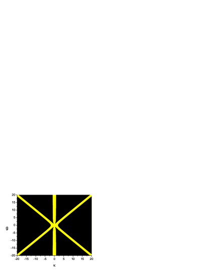
Figure 1: The regions (yellow in the online version) in the parameter plane $\kappa$-$g$ where the photon generation from vacuum is possible.

3 Analysis of special cases

3.1 Expected resonances for $|\kappa|=|g|$

Condition (17) is obviously broken if $|\kappa|=|g|$, i.e. along the bisectrices in figure 1. The possibility of photon generation in this case seems quite natural, as soon as the corresponding modulation frequency $\eta=2(1+\kappa)$ is exactly twice bigger than one of two eigenfrequencies $\omega_{\pm}=1\pm g$ of the stationary part of Hamiltonian (4) (with $\chi_{t}\equiv 0$). Namely, this case was studied for the first time in [4]. In particular, for $|\beta|\ll|g|$ photons can be created if $|\kappa-g|<|\beta|$. Under this condition the solutions to equations (11) have rather simple explicit forms if, in addition, $(\beta t)(\beta/g)\ll 1$:

$$a(t)=\frac{1}{2}\left[\left(a_{0}-b_{0}\right)\cosh(\beta t)+\left(a_{0}^{\dagger}-b_{0}^{\dagger}\right)\sinh(\beta t)\right]e^{igt}+\frac{1}{2}\left(a_{0}+b_{0}\right)e^{-igt},$$ (18)

$$b(t)=\frac{1}{2}\left[\left(b_{0}-a_{0}\right)\cosh(\beta t)+\left(b_{0}^{\dagger}-a_{0}^{\dagger}\right)\sinh(\beta t)\right]e^{igt}+\frac{1}{2}\left(a_{0}+b_{0}\right)e^{-igt}\,.$$ (19)

The mean numbers of quanta in both the modes coincide (for the initial vacuum states):

$$\langle n_{a}(t)\rangle=\langle n_{b}(t)\rangle=\frac{1}{2}\sinh^{2}(\varepsilon t/4).$$ (20)

The photon generation rate in the field mode interacting with the oscillator detector turns out to be twice smaller than for the empty cavity [given by equation (2)]. This result was obtained in [4], but unfortunately the argument of the hyperbolic sine function there was twice bigger due to a misprint. The effect of diminishing the photon generation rate due to the resonance intermode interactions was discovered in [6, 21]. In the most strong form this effect manifests itself in effectively one-dimensional Fabry–Pérot cavities with (quasi)equidistant spectra of eigenfrequencies [4, 22]. For other statistical properties of the field mode, we have the following formulae:

$$\Delta=\frac{1}{4}\cosh^{2}(\beta t),\qquad Q=\frac{1}{2}\cosh(2\beta t)=2\langle n\rangle+\frac{1}{2},$$ (21)

$$\sigma_{xx}=\frac{1}{2}\cosh(\beta t)\left[\cosh(\beta t)+\sinh(\beta t)\cos(2gt)\right],$$ (22)

$$\sigma_{pp}=\frac{1}{2}\cosh(\beta t)\left[\cosh(\beta t)-\sinh(\beta t)\cos(2gt)\right],$$ (23)

$$\sigma_{xp}=\frac{1}{2}\cosh(\beta t)\sinh(\beta t)\sin(2gt).$$ (24)

The minimal value (with respect to fast oscillations with frequency $2g\gg\beta$) of the variance of any of two quadrature components is equal to

$$\sigma_{min}=\frac{1}{4}\left(1+e^{-2\beta t}\right)\to\frac{1}{4}\,.$$ (25)

Formula (5) for the PDF in the field mode can be written in the case involved as (see also [4])

$$f(m)=(iz)^{m}\sqrt{1-3z^{2}}P_{m}(-iz),\qquad z\equiv\frac{\tanh(\beta t)}{\sqrt{4-\tanh^{2}(\beta t)}}\,.$$ (26)

For big values of index $m$, one can use the asymptotical formula for the Legendre polynomials [23]

$$P_{m}(\cosh\xi)\approx\left(\frac{\xi}{\sinh\xi}\right)^{1/2}I_{0}\left(\left[m+1/2\right]\xi\right),$$ (27)

where $I_{0}(z)$ is the modified Bessel function. Taking into account known asymptotical formulae for the Bessel functions of big (complex) arguments and following the scheme described in [17], one can arrive at the formula

$$f(m)\approx\frac{\displaystyle{\frac{[\tanh(\beta t)]^{m}}{[2-\tanh(\beta t)]^{m+\frac{1}{2}}}+\frac{[-\tanh(\beta t)]^{m}}{[2+\tanh(\beta t)]^{m+\frac{1}{2}}}}}{\cosh(\beta t)\sqrt{\pi\left(m+\frac{1}{2}\right)}},$$ (28)

which is valid under the condition $m\gg 1$ for both small and big values of the product $\beta t$. It is worth comparing formula (28) with the strongly oscillating distribution

$$f_{0}(2k)=\frac{\langle n\rangle^{k}(2k)!}{(1+\langle n\rangle)^{k+1/2}(2^{k}k!)^{2}},\quad f_{0}(2k+1)=0$$ (29)

in the squeezed vacuum state arising in the absence of interaction with the detector. The probabilities of observing odd numbers of quanta in the distribution (28 are close to zero if $\beta t\ll 1$. But this case is not very interesting, since $\langle n(t)\rangle\ll 1$ under this condition. In contrast, if $\beta t>1$, so that $\tanh(\beta t)$ is close to unity and $\langle n(t)\rangle\approx\exp(2\beta t)/8$, then one can rewrite (28) as

$$f(m)\approx\displaystyle{\frac{1+(-1)^{m}3^{-m-1/2}}{\sqrt{2\pi m\langle n(t)\rangle}}}\,.$$ (30)

For $m\gg 1$ the second term in the numerator of fraction in formula (30) is very small. Therefore this formula shows very smooth distribution, quite different from (29). Note that for $k\gg 1$ formula (29) can be written (using the Stirling formula for the factorials) as $f_{0}(2k)\approx[\pi k\langle n\rangle]^{-1/2}$. Comparing this expression with (30) for $m=2k$ we see that $f(2k)\approx f_{0}(2k)/2$, so the distribution (30) can be considered as an average of even and odd values of the ‘saw-tooth’ distribution (29). The plots of exact distributions (26) and (29) for $m\leq 20$ and $\langle n\rangle\sim 6$, illustrating these observations, were given in [4].

On the basis of this example, one could suppose that the drastic change of the behavior of the PDF is due to the strong coupling with a detector, which plays a role of some ‘reservoir’ (note that thermal reservoirs usually cause ‘smoothing’ of any oscillatory behavior). However, the examples of the following subsections show that the real situation is more intricate, and even the strong coupling with a detector not always destroys the oscillations of the PDF or some other physical quantities. A rough analogy can be the case of nonthermal ‘rigged’ reservoirs, which can enhance oscillations of some functions.

3.2 Surprising resonance at $\kappa=0$

Figure 1 shows the existence of resonance photon generation for $\kappa=0$ and for any value of the coupling constant $g$. This result, first discovered in [24], seems surprising, because in the absence of detector (for $g=0$) the mean number of quanta in the case of a small detuning $\kappa\neq 0$ is given by the following generalization of formula (2):

$$\langle n_{0}(t)\rangle=\frac{\varepsilon^{2}/4}{\varepsilon^{2}/4-\kappa^{2}}\sinh^{2}\left(t\sqrt{\varepsilon^{2}/4-\kappa^{2}}\right).$$ (31)

Formula (31) shows that the deviation of the modulation frequency from the resonance value $\eta=2$ by $2\kappa=\varepsilon$ stops the photon generation in the empty cavity. Therefore it was natural to expect [4] that for $g\neq 0$, the modulation frequency must be close to $2\omega_{\pm}=2(1\pm g)$, with the deviation not exceeding something of the order of $\varepsilon$. Nonetheless, in reality the photons can be created also for $|\kappa|<|\beta|$ even if $|g|\gg|\beta|$. Perhaps, this happens due to some kind of quantum interference. The solutions of equations of motion (11) with $\kappa=0$ and arbitrary values of $\beta$ and $g$ can be found in [24] (similar equations were solved in the contexts of different other physical problems in [25, 26]). We bring here only some consequences of that solutions. The mean number of quanta in the field mode in the case of $|g|\gg|\beta|$ is equal to (for $\beta t\gg 1$)

$$\langle n(t)\rangle\approx\frac{1}{4}e^{2\beta t}\left[1+\frac{\beta}{\gamma}\sin(2\gamma t)+\frac{2\beta^{2}}{\gamma^{2}}\sin^{2}(\gamma t)\right],$$ (32)

where $\gamma=\sqrt{g^{2}-\beta^{2}}$. Again, the rate of photon generation is roughly twice smaller than in the empty cavity, but the mean photon number is approximately twice bigger than in the case of $\kappa=g$ considered in the preceding subsection. Time dependences of the mean numbers of quanta in the field mode in different regimes are compared in figure 2. The third (blue) line from the left (corresponding to the case of $\kappa=0$) shows remarkable horizontal steps. This peculiar behavior was explained in [24].

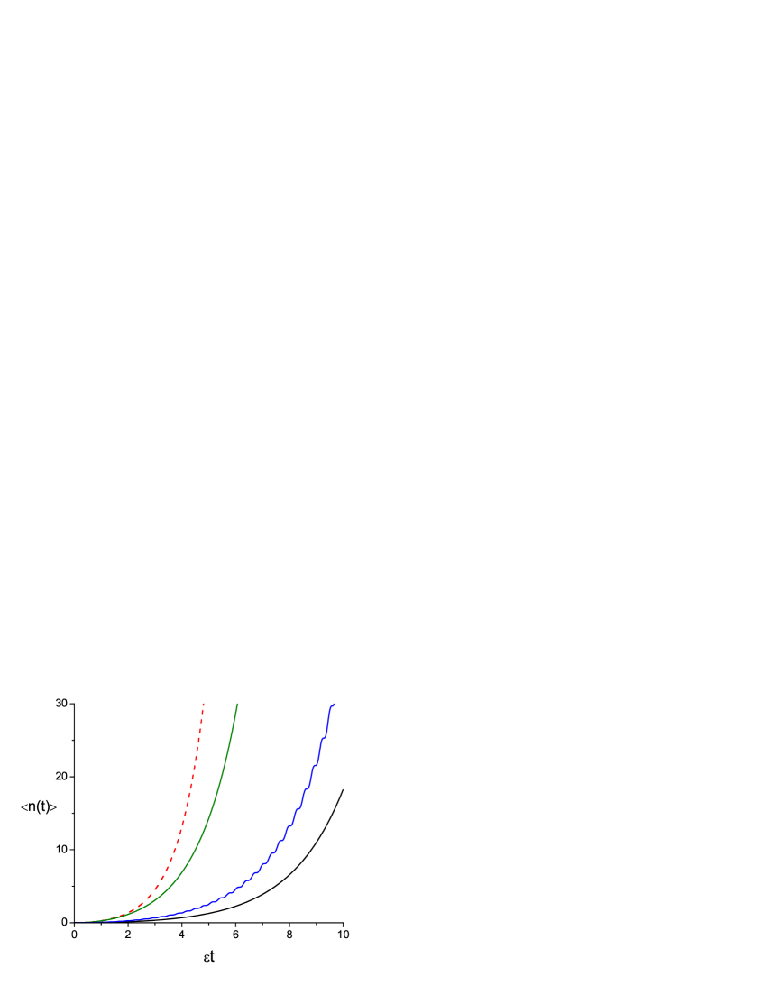
Figure 2: The mean number of quanta in the resonance field mode versus the dimensionless time $\varepsilon t$ for different parameters $\varepsilon$, $g$ and $\kappa$. The order of lines from the left to the right: $g=\kappa=0$, $\varepsilon=10^{-3}$; $\beta=\kappa=g=10^{-2}$ (see subsection 3.3); $\kappa=0$, $g=10\varepsilon=10^{-2}$; $\kappa=g=10^{-2}=10\varepsilon$.

Formula (5) indicates that even-odd oscillations of the PDF can happen if the argument of the Legendre polynomial is close to zero [since $P_{2m+1}(0)=0$ while $P_{2m}(0)=(-1)^{m}(2m-1)!!/(2m)!!$]. In the most strong form these oscillations manifest themselves for pure quantum Gaussian (squeezed) states with $4\Delta-1\equiv 0$, as one can see in formula (29). In the case of $\kappa=0$ we have $4\Delta-1=4g^{2}\beta^{2}\sin^{4}(\gamma t)/\gamma^{4}$, and this quantity is very small if $|g|\gg|\beta|$. Therefore, contrary to the case of $\kappa=g\gg\beta$, the PDF shows oscillations, and for $m\gg 1$ we have

$$f(2m)=\frac{\tanh^{2m}(\beta t)}{\cosh(\beta t)}\frac{(2m-1)!!}{(2m)!!},$$ (33)

$$\frac{f(2m+1)}{f(2m)}=\frac{2(2m+1)\beta^{2}\sin^{4}(\gamma t)}{g^{2}\sinh(2\beta t)}\ll 1.$$ (34)

3.3 The intermediate regime $\kappa=g=\beta$

Another interesting special case admitting explicit solutions is $\beta=\kappa=g$ (the point of intersection of the bisectrice of the first quadrant and the circle $\kappa^{2}+g^{2}=2\beta^{2}$ [see condition (15)] in figure 1). The characteristic values are $\lambda_{1,2}=\pm\sqrt{2}\,\beta$ and $\lambda_{3,4}=\pm i\sqrt{2}\,\beta$, so that the following exact formulae hold ($x=\sqrt{2}\,\beta t$):

$$a(t) = \frac{e^{i\beta t}}{\sqrt{8}}\Bigg{\{}a_{0}\left[\sqrt{8}\,\cosh(x)-i\sinh(x)-i\sin(x)\right]$$

$$+a_{0}^{\dagger}\left[3\sinh(x)+\sin(x)\right]$$

$$+b_{0}\left[\sqrt{2}\,\cos(x)-\sqrt{2}\,\cosh(x)-i\sinh(x)-i\sin(x)\right]$$

$$+b_{0}^{\dagger}\left[\sin(x)-\sinh(x)+i\sqrt{2}\,\cosh(x)-i\sqrt{2}\,\cos(x)\right]\Bigg{\}},$$

$$\langle a^{\dagger}a\rangle=\frac{1}{2}\left[1+3\sinh^{2}(x)+\sinh(x)\sin(x)-\cosh(x)\cos(x)\right].$$ (35)

Despite the presence of trigonometric functions in formula (35), the mean number of photons grows practically exponentially without visible oscillations, as shown by the second line from the left in figure 2. The asymptotical rate of photon generation in this case is equal to $\varepsilon/\sqrt{2}$ – an intermediate value between $\varepsilon$ and $\varepsilon/2$ characterizing the two adjacent curves.

The parameters entering formula (5) for the PDF are as follows:

$$4\Delta-1 = 2\cosh^{2}(x)-2\left[\sinh(x)\sin(x)+\cosh(x)\cos(x)\right]$$

$$-\frac{1}{2}\left[\cosh(x)\sin(x)-\sinh(x)\cos(x)\right]^{2},$$

$$D_{+}=8\cosh^{2}(x)-4\cosh(x)\cos(x)-\frac{1}{2}\left[\cosh(x)\sin(x)-\sinh(x)\cos(x)\right]^{2},$$

$$D_{-}=-4\sinh^{2}(x)-4\sinh(x)\sin(x)-\frac{1}{2}\left[\cosh(x)\sin(x)-\sinh(x)\cos(x)\right]^{2}.$$

For $x\gg 1$ we have

$$4\Delta-1\approx\frac{1}{2}e^{2x}(1-\xi/4),\qquad\xi=(\sin\,x-\cos\,x)^{2},$$

$$D_{+}\approx 2e^{2x}(1-\xi/16),\qquad D_{-}\approx-e^{2x}(1+\xi/8).$$

Consequently,

$$f(m)\approx\sqrt{2}\left(\frac{1+3\xi/16}{2}\right)^{m/2}e^{-x}\,i^{m}P_{m}\left(-\frac{i(1-\xi/4)}{\sqrt{8+\xi/2}}\right).$$

Since $0\leq\xi\leq 2$, the argument of the Legendre polynomial varies from $-i/\sqrt{8}$ to $-i/6$, i.e. it cannot assume very small values. Therefore the PDF does not show noticeable oscillations, and can be well approximated (for $1\ll m\sim\langle n\rangle$) by the formula [17, 27]

$$f(m)\approx\frac{\exp\left[-(2m+1)/(4\langle n\rangle)\right]}{\sqrt{\pi\langle n\rangle(2m+1)}}\,.$$ (36)

The quantity showing oscillations in the case concerned is the invariant squeezing coefficient $S=2\sigma_{min}$. Indeed, since $\Delta\sim\tau\gg 1$ for $x\gg 1$, formula (9) can be simplified as $S\approx 2\Delta/\tau$, so that $S(x\gg 1)\approx(1-\xi/4)/{3}$. Since $\xi(x)$ is a periodic function of time, the minimal quadrature variance $\sigma_{min}$ does not go asymptotically to some limit, but it oscillates between the values $1/6$ and $1/12$.

4 Conclusions

The main results of this paper are as follows. We found the conditions of photon generation in a three-dimensional cavity with resonantly oscillating ideal walls when the resonance field mode is linearly coupled to a detector modeled as harmonic oscillator. The ‘allowed’ and ‘forbidden’ zones in the space of parameters $\varepsilon$, $g$ and $\kappa$ are presented in figure 1. We have shown that the main physical observables, such as the mean number of created quanta, their distribution function and the invariant squeezing coefficient, can show either smooth monotonic behavior or some kinds of oscillations, depending on the parameters characterizing the process. However, the oscillations of different quantities seem to be uncorrelated, according to the examples considered.

References

References

- [1] Dodonov V V 2010 Phys. Scr. 82 038105
- [2] Dalvit D A R, Maia Neto P A and Mazzitelli F D 2011 Casimir Physics (Lecture Notes in Physics Vol 834) ed D Dalvit, P Milonni, D Roberts and F da Rosa (Berlin: Springer) p 419
- [3] Nation P D, Johansson J R, Blencowe M P and Nori F 2012 Rev. Mod. Phys. 84 1–24
- [4] Dodonov V V and Klimov A B 1996 Phys. Rev. A 53 2664–82
- [5] Plunien G, Schützhold R and Soff G 2000 Phys. Rev. Lett. 84 1882–5
- [6] Crocce M, Dalvit D A R and Mazzitelli F D 2001 Phys. Rev. A 64 013808
- [7] Law C K 1994 Phys. Rev. A 49 433–7
- [8] Dodonov V V 1995 Phys. Lett. A 207 126–32
- [9] Braggio C, Bressi G, Carugno G, Del Noce C, Galeazzi G, Lombardi A, Palmieri A, Ruoso G and Zanello D 2005 Europhys. Lett. 70 754–60
- [10] Braggio C, Bressi G, Carugno G, Della Valle F, Galeazzi G and Ruoso G 2009 Nucl. Instr. and Meth. A 603 451–5
- [11] Agarwal G S and Adam G 1988 Phys. Rev. A 38 750–3
- [12] Chaturvedi S and Srinivasan V 1989 Phys. Rev. A 40 6095–8
- [13] Marian P 1992 Phys. Rev. A 45 2044–51
- [14] Marian P and Marian T A 1993 Phys. Rev. A 47 4474–86
-
[15]
Dodonov V V, Man’ko O V and Man’ko V I 1994
Phys. Rev. A 49 2993–3001
Dodonov V V and Man’ko V I 1994 J. Math. Phys. 35 4277–94 - [16] Dodonov V V 2003 Theory of Nonclassical States of Light ed V V Dodonov and V I Man’ko (London: Taylor & Francis) pp 153–218
- [17] Dodonov V V 2010 Phys. Scr. T140 014020
-
[18]
Lukš A, Peřinová V and Hradil Z 1988
Acta Phys. Polon. A 74 713–21
Lukš A, Peřinová V and Peřina J 1988 Opt. Commun. 67 149–51 - [19] Loudon R 1989 Opt. Commun. 70 109–14
- [20] Dodonov V V, Man’ko V I and Polynkin P G 1994 Phys. Lett. A 188 232–8
- [21] Dodonov A V and Dodonov V V 2001 Phys. Lett. A 289 291–300
- [22] Dodonov A V and Dodonov V V 2012 Phys. Lett. A 376 1903–6
- [23] Olver F W J 1974 Asymptotics and Special Functions (New York: Academic Press) p 463
- [24] Dodonov A V and Dodonov V V 2012 Phys. Rev. A 86 015801
- [25] Sete E A and Eleuch H 2010 Phys. Rev. A 82 043810
- [26] Zhang X, Zheng T-Y, Tian T and Pan S-M 2011 Chinese Phys. Lett. 28 064202
- [27] Dodonov V V 2009 Phys. Rev. A 80 023814