Dynamical Transition in Interaction Quenches of the One-Dimensional Hubbard Model

Abstract

We show that the non-equilibrium time-evolution after interaction quenches in the one dimensional, integrable Hubbard model exhibits a dynamical transition in the half-filled case. This transition ceases to exist upon doping. Our study is based on systematically extended equations of motion. Thus it is controlled for small and moderate times; no relaxation effects are neglected. Remarkable similarities to the quench dynamics in the infinite dimensional Hubbard model are found suggesting dynamical transitions to be a general feature of quenches in such models.

I Introduction

In the last years, seminal experimental setups have been developed combining a very good decoupling of the quantum systems from their environment with a high degree of controllability of the system’s parameters. This renders the observation of the temporal evolution of closed quantum systems for long times possible. Switching the internal parameters provides tools to investigate systems out of equilibrium. In optical lattices, the internal parameters such as hopping and particle-particle interaction can be manipulated Greiner et al. (2002a, b); Kinoshita et al. (2006); Bloch et al. (2008). Furthermore, various pumb-probe experiments based on ultrafast spectroscopy Perfetti et al. (2006) have been developed Bloch et al. (2008).

These developments have triggered extensive theoretical studies of physics far from equilibrium, based on a large variety of analytical and numerical tools Anders and Schiller (2005); Cazalilla (2006); Freericks et al. (2006); Kollath et al. (2007); Manmana et al. (2007); Moeckel and Kehrein (2008); Eckstein et al. (2009); Uhrig (2009); Enss and Sirker (2012); Goth and Assaad (2012). The goal is to qualitatively understand and to quantitatively describe the dynamics of quantum systems far from thermal equilibrium. How do such states evolve? Do they relax towards equilibrium? How does this happen and on which time scales?

These issues are relevant in all dimensions. But so far the infinite dimensional and the one-dimensional (1D) case have attracted the greatest interest. Mainly, this is due to the possibility of approximation-free results in both cases. The infinite dimensional case ($d\to\infty$) is amenable by dynamical mean-field theory (DMFT) Metzner and Vollhardt (1989); Müller-Hartmann (1989); Georges et al. (1996) for which it is exact, also in the non-equilibrium case Freericks et al. (2006). The 1D case is amenable to analytical (e.g. bosonization Cazalilla (2006); Uhrig (2009); Dóra et al. (2011); Rentrop et al. (2012)) and numerical (e.g. time-dependent density-matrix renormalization Daley et al. (2004); White and Feiguin (2004); Kollath et al. (2007); Manmana et al. (2007)) approaches. In addition, there is a fascinating conceptual issue inherent to 1D systems: All extended non-trivial integrable quantum systems are 1D and the existence of an exhaustive number of conserved quantities influences the dynamics strongly because it implies a macroscopic number of conserved quantitities Rigol et al. (2007). Still, relaxation in local quantities due to dephasing may occur Barthel and Schollwöck (2008).

One efficient way to realize states far from equilibrium are interaction quenches Barthel and Schollwöck (2008). The interaction value is changed abruptly increasing it Cazalilla (2006); Kollath et al. (2007); Manmana et al. (2007); Moeckel and Kehrein (2008); Uhrig (2009); Dóra et al. (2011) or decreasing it Goth and Assaad (2012). We focus on interactions which are suddenly switched on with Fermi seas as initial states. This simplifies the evaluation because all correlations are known analytically, but it is not essential for the applicability of our approach which is based on extended equations of motion Uhrig (2009).

For an understanding of the dynamics of quenched systems also the behavior on short and moderate times directly after the quench matters. Relaxation, if it happens, may set in directly or coherent oscillations may take place before relaxation occurs on a longer time scale. The occurrence of intermediate time scales, on which the system does not yet reflect the long-time behavior, is subsumed under the term “prethermalization” Berges (2004); Moeckel and Kehrein (2008, 2009). These issues are particularly difficult to study in strongly correlated systems.

Interestingly, evaluating the DMFT equations after interaction quenches of the half-filled system two regimes occurred Eckstein et al. (2009) which are characterized by qualitative differences in the time dependence of the jump $\Delta n(t)$ in the momentum distribution at the Fermi level. For small values of the interaction $U$, this quantity decreases gradually from its initial value of unity corresponding to the non-interacting Fermi sea and a prethermalization plateau can be discerned. For large values of $U$, the jump $\Delta n(t)$ is characterized by strong oscillations. The key difference is that $\Delta n(t)$ displays zeros in the strong-interaction regime while they are absent for weak interaction.

This observation of two qualitatively different dynamics could be retrieved in a variational Gutzwiller approach, evaluated in Gutzwiller approximation, by Schiró and Fabrizio Schiró and Fabrizio (2010). Their treatment maps the quantum dynamics to a classical mechanics problem. True relaxation, however, is neglected in this way. But the resulting equations allow for an analytic evaluation. The oscillatory regime for weak quenches and the one for strong quenches are separated by a singularity indicating a dynamical transition. Note that the Gutzwiller approximation becomes exact for infinite coordination number Metzner and Vollhardt (1988); Gebhard (1990) so that the similarity between the DMFT and the Gutzwiller results may not suprise.

In view of these results, it is our goal to show that a Hubbard model with completely different properties displays essentially the same dynamical transition. Thus we study the one-dimensional Hubbard model. It is different from the Hubbard model examined by DMFT and Gutzwiller techniques in two important aspects: (i) Scattering between the excitations is controlled by momentum conservation in 1D Luther and Peschel (1975); Haldane (1980); Meden and Schönhammer (1992); Voit (1995); Miranda (2003) while momentum conservation is suppressed at internal vertices in large dimensions Metzner and Vollhardt (1989); Müller-Hartmann (1989). (ii) The macroscopic number of conserved quantities in the integrable 1D Hubbard model Essler et al. (2005) should constrain the non-equilibrium dynamics so that it differs significantly from what is seen in higher dimensions. Yet we find that the dynamical transition is also present in 1D with even quantitative similarities.

The article is set up as follows. Next, the model, the quench, and our approach to them are introduced. In Sect. III, the results for the time-dependent jump in the momentum distribution are presented. In Sect. IV, we analyse the data with respect to the occurrence of a dynamical transition. Finally, conclusions are drawn in Sect. V.

II Quenched Hubbard Model

For the quench, we start from a Fermi sea and switch on the interaction abruptly. Thus the Hubbard Hamiltonian becomes time-dependent and reads

$$H_{\text{Hu}}=-J\sum_{\langle i,j;\sigma\rangle}\big{(}\hat{c}_{i,\sigma}^{\dagger}\hat{c}_{j,\sigma}^{\phantom{\dagger}}+\text{h.c.}\big{)}+U(t)\sum_{i}\hat{n}_{i,\uparrow}\hat{n}_{i,\downarrow}$$ (1)

with a local repulsion $U(t)$, where $\hat{c}_{j}^{\dagger}$ ($\hat{c}_{j}^{\phantom{\dagger}}$) create (annihilate) a particle with spin $\sigma$ at site $j$ and $\hat{n}_{j}=\hat{c}_{j}^{\dagger}\hat{c}_{j}^{\phantom{\dagger}}$. We study $U(t)=\Theta(t)U\geq 0$ and define the band width $W=4J$ as the natural energy scale.

The approach used is a systematically controlled expansion of the Heisenberg equations of motion for $\hat{c}_{j,\sigma}^{\dagger}$ Uhrig (2009). By commuting the interacting $H$ after the quench recursively with $\hat{c}_{j,\sigma}^{\dagger}$, i.e., by applying the Liouvillian, we obtain differential equations for the prefactors of the expansion of $\hat{c}_{j,\sigma}^{\dagger}(t)$ in more and more monomials of $\hat{c}_{i,\sigma}^{\dagger}$ and $\hat{c}_{j}^{\phantom{\dagger}}$ at $t=0$. We perform this calculation in real space. The application of one commutation is a ‘loop’. Roughly, each loop multiplies the number of tracked monomials by a factor 3. We are able to realize up to 11 loops. In Fig. 1 the convergence of time-dependent results with the loop number is shown. Our approach bears similarities to recent calculations based on recursively constructed Hilbert spaces Bonča et al. (2007). But we stress that our approach is operator-oriented. The evaluation of expectation values is done only at the end at the time instant of interest.

The evaluation of the differential equations on the one-loop level describes the time dependence of the initial operator $\hat{c}_{j,\sigma}^{\dagger}$ exactly in linear order in $t$. By each loop we increment the depth of the hierarchy of the equations of motions by one and thus the time dependence of the initial operator $\hat{c}_{j,\sigma}^{\dagger}$ is precisely captured up to order $t^{n}$ for $n$ loops. Finally, we solve the differential equations numerically so that also higher powers of $t$ are generated. The conceptual asset of the approach is that it works directly on the infinite lattice by exploiting translational invariance. No relaxation effects occurring up to the considered order are neglected. A quantitative analysis of the convergence of the approach and of its accuracy is presented in App. A.

III Time-dependent jump in the momentum distribution

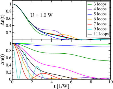
Figure 1: (color online) Upper panel: Jump $\Delta n$(t) for the half-filled Hubbard model for various loop numbers. Lower panel: $\Delta n(t)$ for increasing $U$ (from top to bottom at small $t$: $U/W=0.125,0.25,0.5,0.8,1.0,1.25,1.5,2.0,5.0$) in 11 loops.

We focus on the momentum distribution $n_{k}(t):=\langle\hat{c}_{k,\sigma}^{\dagger}\hat{c}_{k,\sigma}^{\phantom{\dagger}}\rangle(t)$ where $k$ is the wave vector Uhrig (2009). In particular, we study the jump $\Delta n(t):=n_{k_{\text{F}}+0}(t)-n_{k_{\text{F}}-0}(t)$ at the Fermi vector $k_{\text{F}}$ with $\Delta n(0)=1$ for the initial Fermi sea. After the quench, $\Delta n$ shows slow relaxation to zero and damped oscillations. The upper panel of Fig. 1 depicts the jumps for increasing number of loops for the half-filled Hubbard model. Good convergence is obtained for 11 loops up to about $t\approx 10/W$. The precise value up to which the data is reliable depends on the details, see App. A. The lower panel of Fig. 1 displays the data for various values of $U$.

The slow relaxation seen in Fig. 1 is characteristic for a 1D model as can be understood from results for Tomonaga-Luttinger models obtained by bosonization Cazalilla (2006); Uhrig (2009); Dóra et al. (2011); Rentrop et al. (2012). It is found that power laws instead of exponential relaxation occur. Our data agrees with this expectation see data in Ref. Hamerla and Uhrig, 2012.

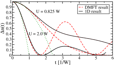
Figure 2: (color online) Jump $\Delta n(t)$ for the half-filled Hubbard model in 1D (black, solid lines) and on the Bethe lattice with infinite coordination number (gray, dashed lines from Ref. Eckstein et al. (2009)). Dotted line: Second order result $\Delta n=1-U^{2}t^{2}/4$.

Our first key observation stems from the comparison of the 1D data with exact DMFT data for a Bethe lattice Eckstein et al. (2009). The common lore expects a crucially distinct behavior due to the differing dimensionality and the integrability of the 1D Hubbard model Essler et al. (2005). The scattering in 1D is strongly restricted due to momentum conservation Luther and Peschel (1975); Haldane (1980); Meden and Schönhammer (1992); Voit (1995); Miranda (2003) while this conservation is irrelevant at internal vertices in DMFT Metzner and Vollhardt (1989); Müller-Hartmann (1989). Yet Fig. 2 shows qualitatively similar results for larger values of $U$. For $U\lessapprox W$ quantitative differences prevail beyond $t=2/W$ so that it is difficult to discern qualitative similarities. But for interaction values beyond the band width $W$ coherent oscillations in $\Delta n(t)$ occur Eckstein et al. (2009) which agree in that the minima appear at almost the same values. To stress that this is not simply an effect of the leading order in $t$ the second order result $\Delta n(t)=1-U^{2}n(2-n)t^{2}/4$ ($n$ filling factor) is included in Fig. 2. The amplitudes of the oscillations, however, differ significantly. We conclude that the periods of the oscillations are a candidate for similarities while the amplitudes and their decay are more strongly depending on the model. In 1D, a slow power law relaxation is generic while exponential relaxation is expected in higher dimensions in agreement with the DMFT data. These striking similarities indicate that for large $U$ the physics is governed by local processes as is explained below.

IV Dynamical transition

We return to the oscillations $\propto\cos(2\pi t/T)$ which appear both for strong quenches and for weak quenches. Schiró and Fabrizio derived an analytic formula for the period $T$ of the oscillations at half-filling

$$T=\left\{\begin{array}[]{lcl}\frac{4\sqrt{2}}{U_{c}}K(2U/U_{c})&\text{for}&U<U_{c}\\ \frac{4}{U_{c}}K(U_{c}/2U)&\text{for}&U>U_{c},\end{array}\right.$$ (2)

where $K(x)$ is the complete elliptic integral of the first kind and $U_{c}$ the value where the Mott transition occurs in the Gutzwiller approach Schiró and Fabrizio (2010). It is given by $-8E_{\text{kin}}$ where $E_{\text{kin}}$ is the kinetic energy of the half-filled Fermi sea. Away from half-filling, the logarithmic singularity in (2) is smeared out.

What does our data yield for the oscillation periods? In absence of relaxation, thus without changes in the oscillatory amplitudes, it is straightforward to read off the period $T$. In our data, this is less obvious. To determine the period $T$ we fit a straight line to the data such that it is a double tangent to two points close to the first two minima, see inset of Fig. 4. From the first instant we deduce the period $T=2t_{0}$. The double tangent is constructed to take into account that the oscillatory part may be small and sit on top of a non-oscillatory relaxation. In case only one minimum can be determined, we read off its instant in time to find $t_{0}$.

Representative results are depicted in Fig. 4 for various fillings. For comparison, the analytic formula (2) is plotted as well. At and around half-filling ($n=1$) and for interaction values $U$ smaller than about $U_{c}/2$ the oscillation period $T$ hardly depends on $U$. The rather flat curve in this regime is in agreement with the semiclassical finding for half-filling (2) although the value of $T$ differs roughly by a factor of two which may not surprise in view of the very different models. Note that $T$ stays finite for $U\to 0$. Its value in this limit depends on the filling. Data for other fillings can be found in App. B and in Figs. 3 and 4 below. We stress that all oscillations in the weak quench regime do no show zeros in $\Delta n(t)$ so that $\Delta n(t)>0$.

For quenches to large $U$ and in particular for $U\to\infty$ the curves for all fillings converge well to the asymptotic behavior $T=2\pi/U$. This value corresponds to Rabi oscillations in the local two-level system which is given by a local singly and doubly occupied site. In other words, the lattice behaves as if it were made up from independent Hubbard atoms in first approximation. This finding stems from the basic two-loop calculation leading to

$$\hat{c}_{0,\uparrow}^{\dagger}(t) =h_{0}(-1,t):\hat{c}_{-1,\uparrow}^{\dagger}:+h_{0}(0,t):\hat{c}_{0,\uparrow}^{\dagger}:$$

$$+h_{0}(1,t):\hat{c}_{1,\uparrow}^{\dagger}:+h_{1}(0,0,0,t):\hat{c}_{0,\uparrow}^{\dagger}\hat{c}_{0,\downarrow}^{\dagger}\hat{c}_{0,\downarrow}^{\phantom{\dagger}}:$$ (3)

where site 0 can be any site on the chain because of translational invariance. The coefficients follow the differential equations

$$\partial_{t}h_{0}(0,t) =-Jih_{0}(-1,t)-Jih_{0}(1,t)$$

$$+U\frac{n}{2}\left(1-\frac{n}{2}\right)ih_{1}(0,0,0,t)$$ (4a)

$$\partial_{t}h_{0}(-1,t) =-Jih_{0}(0,t)$$ (4b)

$$\partial_{t}h_{0}(1,t) =-Jih_{0}(0,t)$$ (4c)

$$\partial_{t}h_{1}(0,0,0,t) =Uih_{0}(0,t)+(1-n)h_{1}(0,0,0,t)$$ (4d)

for the coefficients. This result covers the leading order in $t$ independent of the value of $U$ because the commutation of the interaction part in (1) with the local operators, i.e, those at site 0, in (3) does not yield any other operator term than those that we included. In this sense, the approach used becomes exact for $U\to\infty$. The surrounding lattice sites act as damping bath.

At half-filling, the above differential equations can be solved analytically and we find for the oscillation period $T=2\pi/\sqrt{U^{2}+W^{2}/2}$. For finite doping the numerical solution is easily done. In both cases, $T=2\pi/U$ is the leading order result in an expansion in $1/U$. The equations of motion approach is well-controlled for large values of $U$ because the number of operators generated by commutation with the interaction part does not grow infinitely. Their number is finite for a fixed number of sites involved because the corresponding Hilbert space is finite. The subleading order $W/U^{2}$ is exactly captured if all operators acting on two sites are included which happens in the seven-loop calculation. Clearly, local processes dominate for large values of $U$.

Returning to the two regimes of quenches, we stress that only the oscillations at half-filling display zeros in $\Delta n(t)$ after the strong quenches. For any finite doping ($n\neq 1$) the oscillations persist, but do not reach zero any more in their minima as shown in detail in Fig. 3. Even 2% of doping are sufficient to shift the first minimum from zero upwards to a finite value within numerical accuracy, see right panel in Fig. 3.

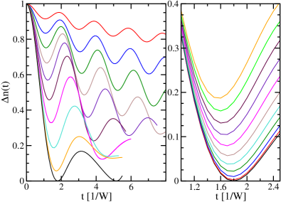
Figure 3: (color online) Oscillations in $\Delta n(t)$ for various dopings. In the left panel, the dopings are from top to bottom at the first minimum: $n=0.1,0.2,0.3,0.4,0.5,0.6,0.7,0.8,0.9,1.0$. In the right panel, the dopings are from top to bottom at the minimum: $n=0.8,0.82,0.84,0.86,0.88,0.9,0.92,0.94,0.96,0.98,1.0$. Clearly, zeros occur only at half-filling.

The regimes of weak and of strong quenches are separated by an anomaly catching the eye in Fig. 4 at $U\approx U_{c}/2$. From our data we cannot identify a singularity because there are some uncertainties in the determination of $T$, see App. C for error bars and further discussion, and we cannot make statement about times beyond $\approx 15/W$. Nevertheless, our finding is suggestive of a singular behavior which may be a jump (indicated by a dashed line) or a logarithmic singularity (the periods rise by about a factor two above their $U\to 0$ value). The similarity to the semiclassical result is surprising and indicates that indeed the two regimes of quenches are separated by a dynamical transition. The small shift of the position of the anomaly from $U=U_{c}/2$ to $U\approx 0.43U_{c}$ is of minor importance.

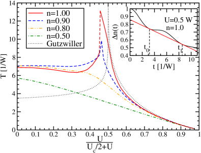
Figure 4: (color online) Period of the oscillations in $\Delta n(t)$ as function of $U$ ($U_{c}=8W/\pi$ in 1D); $n$ denotes the total filling factor per site. The dotted curve depicts the semiclassical Gutzwiller result (2) Schiró and Fabrizio (2010).

We emphasize that all oscillations after strong quenches, to the right of the dashed part of the half-filled curve, display zeros $\Delta n(t)$ while no zeros are found for weak quenches, to the left of the dashed part. This holds, however, only at half-filling. For finite doping, even strong quenches do not imply zeros so that the transition ceases to exist for any doping, see Fig. 3. Thus the data constitutes very strong evidence for a qualitative, dynamical transition between both regimes at half-filling. At finite doping, it appears to be washed out immediately. The anomaly, however, disappears gradually: We see in Fig. 4 that about 20% of doping are required to make the anomaly vanish completely, cf. App. B.

The finding agrees with the semiclassical, relaxation-free Gutzwiller result in infinite dimensions Schiró and Fabrizio (2010) and with the available DMFT data Eckstein et al. (2009). Since such similar behavior occurs in extreme cases such as a one-dimensional integrable model with important momentum conservation and an infinite dimensional model with suppressed momentum conservation the conclusion suggests itself that the dynamical transition is a general feature in quenched, half-filled Hubbard models.

V Conclusions

Summarizing, we studied interaction quenches in the one-dimensional Hubbard model by an approach based on equations of motion. It is systematically controlled in the depth of the hierarchy; here up to 11 commutations were carried out. The accuracy of the data is systematically controlled by the comparison of the results for different loop numbers.

We analyse the time-dependence of the jump in the momentum distribution starting from the initial Fermi sea. Slowly decaying oscillations are found. At half-filling, two qualitatively different regimes appear: For strong quenches, the jumps display zeros, for weak quenches they do not. In the dependence of the oscillation period $T$ on the interaction $U$ a clear anomaly appears separating both regimes. It indicates a dynamical transition. Since this scenario is in surprising agreement with previous findings in infinite-dimensional models Eckstein et al. (2009); Schiró and Fabrizio (2010) we suggest that this scenario holds for half-filled Hubbbard models in general.

Appendix A Technicalities

We are interested in momentum distributions after interaction quenches. They can be computed by Fourier transformation of the one-particle equal time propagators

$$G(\vec{r},t)=\langle\text{FS}|\hat{c}(\vec{r},t)^{\phantom{\dagger}}\hat{c}^{\dagger}(0,t)|\text{FS}\rangle$$ (5)

where the expectation value is taken with respect to the noninteracting Fermi sea $|\text{FS}\rangle$ which represents the initial state before the quench. The $\vec{r}$ stands for a site on the lattice under study, here a chain in one dimension (1D). The time-dependent operators $\hat{c}$ and $\hat{c}^{\dagger}$ are represented by the following ansatz

$$\hat{c}^{\dagger}(\vec{r},t)=\hat{T}_{\vec{r}}^{\dagger}+\left(\hat{T}^{\dagger}\hat{T}^{\dagger}\hat{L}^{\dagger}\right)_{\vec{r}}+...$$ (6)

where $\hat{T}^{\dagger}$ ($\hat{L}^{\dagger}$) denote various superpositions of particle (hole) creation operators. For instance, the single particle creation $\hat{T}^{\dagger}$ is given by

$$\hat{T}_{\vec{r}}^{\dagger}=\sum_{|\vec{\delta}|\lessapprox v_{\text{max}}t}\sum_{\sigma}h_{0}(\vec{\delta},t)\hat{c}_{\vec{r}+\vec{\delta},\sigma}^{\dagger}$$ (7)

with time-dependent prefactors $h_{0}(\vec{\delta},t)$. The shifts $\vec{\delta}$ can be bounded from above by $v_{\text{max}}t$ where $v_{\text{max}}$ is the maximal velocity in the sense of the Lieb-Robinson theorem Lieb and Robinson (1972); Calabrese and Cardy (2006). Physically, this means that there is a maximum velocity with which the essential effects of the Hamiltonian after the quench can travel. Of course, exponentially small effects will be neglected. Hence, in order to describe the dynamics correctly up a certain time one has to include processes up to a certain spatial range Uhrig (2009). This idea is also used in other approaches Enss and Sirker (2012).

To calculate the time dependence of the prefactors we use the Heisenberg equation $\partial_{t}\hat{{A}}(\vec{r},t)=i\left[\hat{{H}},\hat{{A}}(\vec{r},t)\right]$ for the time derivative of an operator $\hat{A}$. On calculating the commutator $\left[\hat{{H}},\hat{c}^{\dagger}(\vec{r},t)\right]$ we encounter two cases. The commutation of the noninteracting part of the Hamiltonian $\hat{{H}}_{0}$ leads to a shift of the fermionic operators in space, whereas the commutation with the interaction term $\hat{{H}}_{\text{int}}$ may additionally create or annihilate particle-hole pairs $\hat{T}^{\dagger}\hat{L}^{\dagger}$. Iterating this process then leads to the ansatz (6). With each commutation more terms with higher number of particles involved are created. Thus the amount of terms grows exponentially: At 11 loops we deal with up to $5\cdot 10^{5}$ monomials in the Hubbard model and a set of differential equations with about $2\cdot 10^{7}$ terms on the right hand side.

The differential equations of the prefactors can be solved numerically with the initial conditions $h_{0}(0,0)=1$ and $h_{i}(\vec{r},t)=0\;\forall i\neq 0$ . Because each commutation comprises one order in time $t$ a calculation with $n$ commutations provides results for $\hat{c}^{\dagger}(t)$ which are exact up to order $t^{n}$. We stress, however, that we do not use a series expansion in $t$ but solve the (truncated) set of differential equations numerically.

Due to the proliferating number of additional terms arising within the calculation we have to restrict ourselves to a finite number of commutations. As terms appearing during the last commutation for the first time lead to an overestimation of the weight loss for the one particle terms, we omit them to improve the convergence. A calculation with $m$ commutations performed in this way is called an $m$-loop calculation.

To illustrate how each commutation improves the result the absolute difference between an $m$-loop calculation and the $11$-loop calculation is shown for a quench with $U=1.0W$ in a double logarithmic plot in Fig. 5. Based on this difference a runaway time is defined as the time $t$ beyond which the difference takes values larger than a certain threshold which we set to $0.01$. This threshold is depicted in Fig. 5 as dashed line.

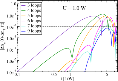
Figure 5: (color online) Absolute difference of the jump $\Delta n_{m}(t)$ at various numbers of loops $m$ relative to the $11$-loop result $\Delta n_{11}(t)$ for the half-filled Hubbard model. Dashed line: Threshold for the determination of the runaway time.

The resulting inverse runaway time is shown in Fig. 6 as function of $\frac{1}{m}$ where $m$ denotes the number of loops performed as described above. The curve shows a power law increase of the runaway time as function of $\frac{1}{m}$, i.e., a power law decrease of the inverse runaway time, with an exponent of about $1.8$. Note that this indicates that the converence is superlinear which is favorable for its application in practical calculations.

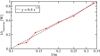
Figure 6: (color online) Double logarithmic plot of the inverse runaway time vs. the inverse number of loops of the corresponding calculation. Dashed line: Power law fit of the data with an exponent of about $1.8$.

Appendix B Oscillations for Various Filling Factors

The period of oscillations for various values of the filling is shown in Fig. 7 as function of the compactified interaction $\frac{U}{(U_{c}/2)+U}$. The interaction $U_{c}$ denotes the values of the Hubbard interaction, where the Mott transition occurs in the Gutzwiller approximation Brinkman and Rice (1970); Metzner and Vollhardt (1988); Gebhard (1990); Schiró and Fabrizio (2010). It takes the value $8W/\pi$ in 1D.

Upon doping the anomaly at $U\approx U_{c}/2$ is gradually reduced until it vanishes completely at around $n\approx 0.8$, leaving behind a monotonic behavior of the period. In contrast to the gradual disappearance of the anomaly, the zeros for strong quenches to the right side of the anomaly vanish immediately upon doping. This was illustrated in Fig. 3.

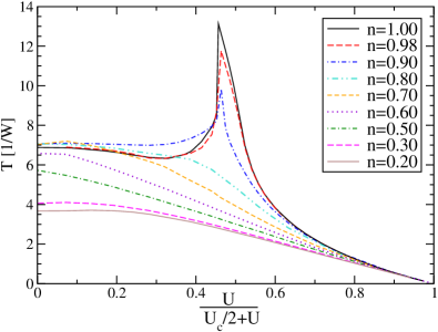
Figure 7: (color online) Period of the oscillations in $\Delta n(t)$ as function of $U$ ($U_{c}=8W/\pi$ in 1D); $n$ denotes the total filling factor per site.

Appendix C Systematic Errors in the Determination of the Period

In the determination of the periods of oscillation systematic inaccuracies due to the finite amount of loops occur. There are two main sources: (i) The finite number of loops and (ii) the way the period $T$ is extracted from the data. The effect of the finite number of loops is estimated by comparing results from the calculation with 11 loops with calculations with a smaller number of loops. This yields estimate (i) for the systematic error.

In order to estimate the effect of the fitting procedure we compare the periods $T$ determined from the double tangents described in the main article to an alternative analysis. In this alternative procedure we read off the positions $t_{0}^{\prime}$ of the first minimum of $\Delta n(t)$ and deduce $T^{\prime}=2t_{0}^{\prime}$. The absolute value $|T-T^{\prime}|$ yields estimate (ii) for the systematic error.

Finally, the maximum of both estimates (i) and (ii) is used as the error of the period. These errors are shown by error bars for fillings $n=1.0,0.8$ and $0.5$ for some exemplary values of the interaction in Fig. 8. In the regime of large interactions, the errors are negligible. Around the anomaly, they are largest as could be expected. But the position and shape of the anomaly are hardly affected by the systematic errors. Thus we are confident that our conclusions are valid.

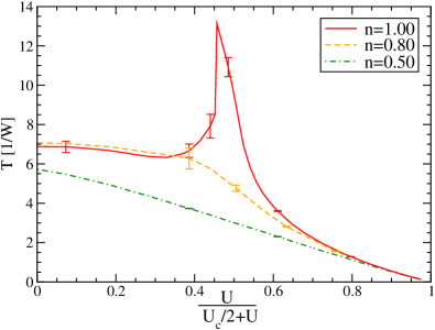
Figure 8: (color online) Period of the oscillations for the fillings $n=1.0,0.8,0.5$. The error bars depict the error of the calculated period for some exemplary values of the interaction. They are estimated as described in the main text.

If a double tangent can be constructed as in the inset of Fig. 3 in the main article, a third way to determine the period is by $T^{\prime\prime}=t_{1}-t_{0}$. This procedure is not possible for all points so that we do not use it for the determination of the curves $T(U)$. For small values of $U$, the third approach yields periods shorter by up to $1/W$.

References

- Greiner et al. (2002a) M. Greiner, O. Mandel, T. Esslinger, T. W. Hänsch, and I. Bloch, Nature 415, 39 (2002a).
- Greiner et al. (2002b) M. Greiner, O. Mandel, T. W. Hänsch, and I. Bloch, Nature 419, 39 (2002b).
- Kinoshita et al. (2006) T. Kinoshita, T. Wenger, and D. S. Weiss, Nature 440, 900 (2006).
- Bloch et al. (2008) I. Bloch, J. Dalibard, and W. Zwerger, Rev. Mod. Phys. 80, 885 (2008).
- Perfetti et al. (2006) L. Perfetti et al., Phys. Rev. Lett. 97, 067402 (2006).
- Anders and Schiller (2005) F. B. Anders and A. Schiller, Phys. Rev. Lett. 95, 196801 (2005).
- Cazalilla (2006) M. A. Cazalilla, Phys. Rev. Lett. 97, 156403 (2006).
- Freericks et al. (2006) J. K. Freericks, V. M. Turkowski, and V. Zlatic, Phys. Rev. Lett. 97, 266408 (2006).
- Kollath et al. (2007) C. Kollath, A. M. Läuchli, and E. Altman, Phys. Rev. Lett. 98, 180601 (2007).
- Manmana et al. (2007) S. R. Manmana, S. Wessel, R. M. Noack, and A. Muramatsu, Phys. Rev. Lett. 98, 210405 (2007).
- Moeckel and Kehrein (2008) M. Moeckel and S. Kehrein, Phys. Rev. Lett. 100, 175702 (2008).
- Eckstein et al. (2009) M. Eckstein, M. Kollar, and P. Werner, Phys. Rev. Lett. 103, 056403 (2009).
- Uhrig (2009) G. S. Uhrig, Phys. Rev. A 80, 061602(R) (2009).
- Enss and Sirker (2012) T. Enss and J. Sirker, New J. Phys. 95, 023008 (2012).
- Goth and Assaad (2012) F. Goth and F. F. Assaad, Phys. Rev. B 85, 085129 (2012).
- Metzner and Vollhardt (1989) W. Metzner and D. Vollhardt, Phys. Rev. Lett. 62, 324 (1989).
- Müller-Hartmann (1989) E. Müller-Hartmann, Z. Phys. B 74, 507 (1989).
- Georges et al. (1996) A. Georges, G. Kotliar, W. Krauth, and M. J. Rozenberg, Rev. Mod. Phys. 68, 13 (1996).
- Dóra et al. (2011) B. Dóra, M. Haque, and G. Zaránd, Phys. Rev. Lett. 106, 156406 (2011).
- Rentrop et al. (2012) J. Rentrop, D. Schuricht, and V. Meden, New J. Phys. 14, 075001 (2012).
- Daley et al. (2004) A. J. Daley, C. Kollath, U. Schollwöck, and G. Vidal, J. Stat. Mech. 2004, P04005 (2004).
- White and Feiguin (2004) S. R. White and A. E. Feiguin, Phys. Rev. Lett. 93, 076401 (2004).
- Rigol et al. (2007) M. Rigol, V. Dunjko, V. Yurovsky, and M. Olshanii, Phys. Rev. Lett. 98, 050405 (2007).
- Barthel and Schollwöck (2008) T. Barthel and U. Schollwöck, Phys. Rev. Lett. 100, 100601 (2008).
- Berges (2004) J. Berges, AIP Conf. Proc. 739, 3 (2004).
- Moeckel and Kehrein (2009) M. Moeckel and S. Kehrein, Ann. of Phys. 324, 2146 (2009).
- Schiró and Fabrizio (2010) M. Schiró and M. Fabrizio, Phys. Rev. Lett. 105, 076401 (2010); ibid. Phys. Rev. B 83, 165105 (2011).
- Metzner and Vollhardt (1988) W. Metzner and D. Vollhardt, Phys. Rev. B 37, 7382 (1988).
- Gebhard (1990) F. Gebhard, Phys. Rev. B 41, 9452 (1990).
- Luther and Peschel (1975) A. Luther and I. Peschel, Phys. Rev. B 12, 3908 (1975).
- Haldane (1980) F. D. M. Haldane, Phys. Rev. Lett. 45, 1358 (1980).
- Meden and Schönhammer (1992) V. Meden and K. Schönhammer, Phys. Rev. B 46, 15753 (1992).
- Voit (1995) J. Voit, Rep. Prog. Phys. 58, 977 (1995).
- Miranda (2003) E. Miranda, Braz. J. Phys. 33, 3 (2003).
- Essler et al. (2005) F. H. L. Essler, H. Frahm, F. Göhmann, A. Klümper, and V. E. Korepin, The One-Dimensional Hubbard Model (Cambridge University Press, UK, 2005).
- Bonča et al. (2007) J. Bonča, S. Maekawa, and T. Tohyama, Phys. Rev. B 76, 035121 (2007).
- Hamerla and Uhrig (2012) S. A. Hamerla and G. S. Uhrig, arXiv/1207.2006v1 This is a preliminary version in the editing process; but the numerical data is in its final form
- Lieb and Robinson (1972) E. H. Lieb and D. W. Robinson, Commun. Math. Phys. 28, 251 (1972).
- Calabrese and Cardy (2006) P. Calabrese and J. Cardy, Phys. Rev. Lett. 96, 136801 (2006).
- Brinkman and Rice (1970) W. F. Brinkman and T. M. Rice, Phys. Rev. B 2, 1324 (1970).