Size distribution of particles in Saturn’s rings from aggregation and fragmentation

Abstract

Saturn’s rings consist of a huge number of water ice particles, with a tiny addition of rocky material. They form a flat disk, as the result of an interplay of angular momentum conservation and the steady loss of energy in dissipative inter-particle collisions. For particles in the size range from a few centimeters to a few meters, a power-law distribution of radii, $\sim r^{-q}$ with $q\approx 3$, has been inferred; for larger sizes, the distribution has a steep cutoff. It has been suggested that this size distribution may arise from a balance between aggregation and fragmentation of ring particles, yet neither the power-law dependence nor the upper size cutoff have been established on theoretical grounds. Here we propose a model for the particle size distribution that quantitatively explains the observations. In accordance with data, our model predicts the exponent $q$ to be constrained to the interval $2.75\leq q\leq 3.5$. Also an exponential cutoff for larger particle sizes establishes naturally with the cutoff-radius being set by the relative frequency of aggregating and disruptive collisions. This cutoff is much smaller than the typical scale of micro-structures seen in Saturn’s rings.

Bombardment of Saturn’s rings by interplanetary meteoroids [1, 2, 3] and the observation of rapid processes in the ring system [4] indicate that the shape of the particle size distribution is likely not primordial or a direct result from the ring creating event. Rather, ring particles are believed to be involved in an active accretion-destruction dynamics [5, 6, 7, 8, 9, 10, 11, 12, 13] and their sizes vary over a few orders of magnitude as a power-law [14, 15, 16, 17], with a sharp cutoff for large sizes [18, 19, 20, 21]. Moreover, tidal forces fail to explain the abrupt decay of the size distribution for house-sized particles [22]. One would like to understand: (i) can the interplay between aggregation and fragmentation lead to the observed size distribution, and (ii) is this distribution peculiar for Saturn’s rings, or is it universal for planetary rings in general? To answer these questions quantitatively, one needs to elaborate a detailed model of the kinetic processes in which the rings particles are involved. Here we develop a theory that quantitatively explains the observed properties of the particle size distribution and show that these properties are generic for a steady-state, when a balance between aggregation and fragmentation holds. Our model is based on the hypothesis that collisions are binary and that they may be classified as aggregative, restitutive or disruptive (including collisions with erosion); which type of collision is realized depends on the relative speed of colliding particles and their masses. We apply the kinetic theory of granular gases [23, 24] for the multi-component system of ring particles to quantify the collision rate and the type of collision.

1 Significance

Although it is well accepted that the particle size distribution in Saturn’s rings is not primordial, it remains unclear whether the observed distribution is unique or universal. That is, whether it is determined by the history of the rings and details of the particle interaction, or if the distribution is generic for all planetary rings. We show that a power-law size distribution with large-size cutoff, as observed in Saturn’s rings, is universal for systems where a balance between aggregation and disruptive collisions is steadily sustained. Hence, the same size distribution is expected for any ring system where collisions play a role, like the Uranian rings, the recently discovered rings of Chariklo and Chiron, and possibly rings around extrasolar objects.

2 Results and Discussion

2.1 Model

Ring particles may be treated as aggregates built up of primary grains [9] of a certain size $r_{1}$ and mass $m_{1}$. Denote by $m_{k}=km_{1}$ the mass of ring particles of ”size” $k$ containing $k$ primary grains, and by $n_{k}$ their density. For the purpose of a kinetic description we assume that all particles are spheres; then the radius of an agglomerate containing $k$ monomers is $r_{k}=r_{1}k^{1/3}$. Systems composed of spherical particles may be described in the framework of the Enskog-Boltzmann theory [25, 26, 27]. In this case the rate of binary collisions depends on particle dimension and relative velocity. The cross-section for the collision of particles of size $i$ and $j$ can be written as $\sigma^{2}_{ij}=\left(r_{i}+r_{j}\right)^{2}=r_{1}^{2}(i^{1/3}+j^{1/3})^{2}$. The relative speed (on the order of $0.01-0.1\,{\rm cm/s}$ [16]) is determined by the velocity dispersions $\left<{\bf v}_{i}^{2}\right>$ and $\left<{\bf v}_{j}^{2}\right>$ for particles of size $i$ and $j$. The velocity dispersion quantifies the root mean square deviation of particle velocities from the orbital speed ($\sim 20\,{\rm km/s}$). These deviations follow a certain distribution, implying a range of inter-particle impact speeds, and thus, different collisional outcomes. The detailed analysis of an impact shows that for collisions at small relative velocities, when the relative kinetic energy is smaller than a certain threshold energy, $E_{\rm agg}$, particles stick together to form a joint aggregate [28, 11, 29]. This occurs because adhesive forces acting between ice particles’ surfaces are strong enough to keep them together. For larger velocities, particles rebound with a partial loss of their kinetic energy. For still larger impact speeds, the relative kinetic energy exceeds the threshold energy for fragmentation, $E_{\rm frag}$, and particles break into pieces [29].

Using kinetic theory of granular gases one can find the collision frequency for all kinds of collisions and the respective rate coefficients: $C_{ij}$ for collisions leading to merging and $A_{ij}$ for disruptive collisions. The coefficients $C_{ij}$ give the number of aggregates of size $(i+j)$ forming per unit time in a unit volume as a result of aggregative collisions involving particles of size $i$ and $j$. Similarly, $A_{ij}$ quantify disruptive collisions, when particles of size $i$ and $j$ collide and break into smaller pieces. These rate coefficients depend on masses of particles, velocity dispersions and threshold energies, $E_{\rm agg}$ and $E_{\rm frag}$:

$$C_{ij}=\nu_{ij}\left(1-\left(1+B_{ij}E_{\rm agg}\right)\exp\left(-B_{ij}E_{\rm agg}\right)\right)$$

$$A_{ij}=\nu_{ij}\exp\left(-B_{ij}E_{\rm frag}\right)$$

$$\nu_{ij}=4\sigma_{ij}^{2}\sqrt{\pi\left(\left<{\bf v}_{i}^{2}\right>+\left<{\bf v}_{j}^{2}\right>\right)/6}$$ (1)

$$B_{ij}=3\,\frac{m_{i}^{-1}+m_{j}^{-1}}{\langle v_{i}^{2}\rangle+\langle v_{j}^{2}\rangle}\,.$$

These results follow from the Boltzmann equation which describes evolution of a system in terms of the joint size-velocity distribution function (see the section below and SI Appendix). The governing rate equations for the concentrations of particles of size $k$ read:

$$\frac{dn_{k}}{dt} = \frac{1}{2}\!\sum_{i+j=k}C_{ij}n_{i}n_{j}-\sum_{i=1}^{\infty}C_{ki}n_{i}n_{k}$$

$$- \sum_{i=1}^{\infty}A_{ki}n_{i}n_{k}\left(1-\delta_{k1}\right)+\sum_{i=1}^{k}n_{i}\sum_{j=k+1}^{\infty}A_{ij}n_{j}x_{k}\left(j\right)$$

$$+ \frac{1}{2}\sum_{i,j\geq k+1}A_{ij}n_{i}n_{j}\left[x_{k}(i)+x_{k}(j)\right]\,.$$

The first term on the right-hand side of Eq. (2.1) describes the rate at which aggregates of size $k$ are formed in aggregative collisions of particles $i$ and $j$ (the factor $\frac{1}{2}$ avoids double counting). The second and third terms give the rates at which the particles of size $k$ disappear in collisions with other particles of any size $i$, due to aggregation and fragmentation, respectively. The fourth and fifth terms account for production of particles of size $k$ due to disruption of larger particles. Here $x_{k}(i)$ is the total number of debris of size $k$, produced in the disruption of a projectile of size $i$. We have analyzed two models for the distribution of debris $x_{k}(i)$. One is the complete fragmentation model, $x_{k}(i)=i\delta_{1k}$, when both colliding particles disintegrate into monomers; another is a power-law fragmentation model, when the distribution of debris sizes obeys a power-law, $x_{k}(i)\sim B(i)k^{-\alpha}$, in agreement with experimental observations, see e.g. [30, 31]; the impact of collisions with erosion is also analysed.

2.2 Decomposition into monomers

In the case of complete fragmentation, $x_{k}(i)=i\delta_{1k}$, the general kinetic equations (2.1) become

$$\frac{dn_{k}}{dt} = \frac{1}{2}\sum_{i+j=k}C_{ij}n_{i}n_{j}-\sum_{i\geq 1}\left(C_{ik}+A_{ik}\right)n_{i}n_{k}$$ (3)

$$\frac{dn_{1}}{dt} = -n_{1}\sum_{j\geq 1}C_{1j}n_{j}+n_{1}\sum_{j\geq 2}jA_{1j}n_{j}$$

$$+ \frac{1}{2}\sum_{i,j\geq 2}A_{ij}(i+j)n_{i}n_{j}\,.$$

Mathematically similar equations modeling a physically different setting (e.g., fragmentation was assumed to be spontaneous and collisional) have been analyzed in the context of rain drop formation [32].

Constant rate coefficients. The case of constant $C_{ij}=C_{0}$ and $A_{ij}=\lambda C_{0}$ can be treated analytically, providing useful insight into the general structure of solutions of Eqs. (3)–(2.2), explicitly showing the emergence of the steady state. The constant $\lambda$ here characterizes the relative frequency of disruptive and aggregative collisions. Without loss of generality we set $C_{0}=1$. Solving the governing equations for mono-disperse initial conditions, $n_{k}(t=0)=\delta_{k,1}$, one finds

$$n_{1}(t)=\lambda_{1}\left[1+\lambda^{-1}\left(\lambda_{2}^{-1}e^{\lambda t}-\lambda^{-1}/2\right)^{-\lambda_{2}/\lambda_{1}}\right]\,,$$ (5)

where $\lambda_{1}=\lambda/(1+\lambda)$ and $\lambda_{2}=2\lambda/(1+2\lambda)$. Utilizing the recursive nature of Eqs. (3), one can determine $n_{k}(t)$ for $k>1$. The system demonstrates a relaxation behavior: After a relaxation time that scales as $\lambda^{-1}$, the system approaches to a steady state with $n_{1}=\lambda_{1}$, the other concentrations satisfying

$$0=\frac{1}{2}\sum_{i+j=k}n_{i}n_{j}-(1+\lambda)n_{k}N.$$ (6)

Here $N=\lambda_{2}$ is the steady-state value of the total number density of aggregates, $N=\sum_{k\geq 1}n_{k}$. We solve (6) using the generation function technique to yield

$$n_{k}=\frac{N}{\sqrt{4\pi}}\left(1+\lambda\right)\left[\frac{2n_{1}}{(1+\lambda)N}\right]^{k}\,\frac{\Gamma(k-\frac{1}{2})}{\Gamma(k+1)}\,.$$ (7)

Now we assume that disruptive collisions in rings are considerably less frequent than aggregative ones, so that $\lambda\ll 1$ (this assumption leads to results that are consistent with observations); moreover, $k\gg 1$ for most of the ring particles. Using the steady-state values, $n_{1}=\lambda_{1}$ and $N=\lambda_{2}$, one can rewrite Eq. (7) for $k\gg 1$ as

$$n_{k}=\frac{\lambda}{\sqrt{\pi}}\,e^{-\lambda^{2}k}\,k^{-3/2}\,.$$ (8)

Thus for $k<\lambda^{-2}$, the mass distribution exhibits power-law behavior, $n_{k}\sim k^{-3/2}$, with an exponential cutoff for larger $k$.

Size-dependent rate coefficients. For a more realistic description, one must take into account the dependence of the rate coefficients on the aggregate size (Eqs. (2.1)). Here we present the results for two basic limiting cases that reflect the most prominent features of the system:

1. The first case corresponds to energy equipartition, $\left<E_{k}\right>=\frac{1}{2}m_{k}\left<{\bf v}_{k}^{2}\right>={\rm const}$, which implies that the energy of random motion is equally distributed among all species, like in molecular gases. In systems of dissipatively colliding particles, like planetary rings, this is usually not fulfilled, the smaller particles being colder than suggested by equipartition [33, 34]. We also assume that the threshold energies of aggregation and fragmentation are constant: $E_{\rm agg}={\rm const}$ and $E_{\rm frag}={\rm const}$; the latter quantities may be regarded as effective average values for all collisions. Then, as it follows from Eqs. (2.1), we have $\lambda=A_{ij}/C_{ij}=\rm const$, and the kinetic coefficients read

$$C_{ij}=C_{0}\left(i^{1/3}+j^{1/3}\right)^{2}\left(i^{-1}+j^{-1}\right)^{1/2}\,,$$ (9)

where $C_{0}=\rm const$, so that the $C_{ij}$ are homogeneous functions of the masses of colliding particles

$$C_{ai,aj}=a^{\varkappa}C_{ij}\,.$$ (10)

The specific form (9) implies that the homogeneity degree is $\varkappa=1/6$.

2. The second limiting case corresponds to equal velocity dispersion for all species, $\left<{\bf v}_{i}^{2}\right>={\bf v}_{0}^{2}={\rm const}$. In planetary rings the smaller particles do have larger velocity dispersions than the larger ones but they are by far not as hot as equipartition would imply [33]. Thus, this limiting case of equal velocity dispersions is closer to the situation in the rings. For the dependence of the fragmentation threshold energy $E_{\rm frag}$ on the masses of colliding aggregates we employ the symmetric function $E_{{\rm frag}}=E_{0}\frac{ij}{i+j}$, which implies that $E_{{\rm frag}}$ is proportional to the reduced mass of the colliding pair, $\mu_{ij}=m_{1}\frac{ij}{i+j}$. This yields $B_{ij}E_{\rm frag}=\left(\frac{3E_{0}}{2m_{1}{\bf v}_{0}^{2}}\right)=\rm const$ and allows a simplified analysis. We assume that the aggregation threshold energy $E_{{\rm agg}}$ for all colliding pairs is large compared to the average kinetic energy of the relative motion of colliding pairs, $\frac{1}{2}\mu_{ij}{\bf v}_{0}^{2}$ (our detailed analysis confirms this assumption, see the SI Appendix). Then $\exp(-B_{ij}E_{\rm agg})\ll 1$ and Eqs. (2.1) yield $C_{ij}=\nu_{ij}$. Therefore the ratio $A_{ij}/C_{ij}=\exp(-B_{ij}E_{\rm frag})$ is again constant. Thus the relative frequency of disruptive and aggregative collisions is also characterized by the constant $\lambda=A_{ij}/C_{ij}$. The kinetic coefficients attain now the form

$$C_{ij}=\tilde{C}_{0}\left(i^{1/3}+j^{1/3}\right)^{2},$$ (11)

which is again a homogeneous function of $i$ and $j$ but with different homogeneity degree $\varkappa=2/3$.

An important property of the kinetic equations, where the rate coefficients $C_{ij}$ and $A_{ij}=\lambda C_{ij}$ are homogeneous functions of $i$ and $j$, is that these equations possess a scaling solution for $i,j\gg 1$. The latter is determined by the homogeneity degree $\varkappa$ and is practically insensitive to the detailed form of these coefficients [35, 36]. We use this property and replace the original rate coefficients (9) and (11) by the generalized product kernel

$$C_{ij}=\widehat{C}_{0}(ij)^{\mu}\qquad\qquad\widehat{C}_{0}=\rm const$$ (12)

For this kernel, the homogeneity degree is $\varkappa=2\mu$. To match it with the homogeneity degree of (9) and (11) we choose $\mu=1/12$ for the first limiting case and $\mu=1/3$ for the second. The advantage of the product kernel (12) is the existence on an analytic solution for the steady state distribution. Indeed, with the homogeneous coefficients (12) the steady-state version of Eqs. (3) reads,

$$0=\frac{1}{2}\sum_{i+j=k}l_{i}l_{j}-(1+\lambda)l_{k}L$$ (13)

where we have used the shorthand notations

$$l_{k}=k^{\mu}n_{k},\qquad\qquad L=\sum_{k\geq 1}l_{k}\,.$$ (14)

With the substitute, $n_{k}\to l_{k}$ and $N\to L$, the system of equations (13) is mathematically identical to the system of equations with a constant kernel (6), so that the steady-state solution reads,

$$n_{k}=\frac{L}{2\sqrt{\pi}}\,e^{-\lambda^{2}k}\,k^{-3/2-\mu}\,,$$ (15)

again a power-law dependence with exponential cutoff.

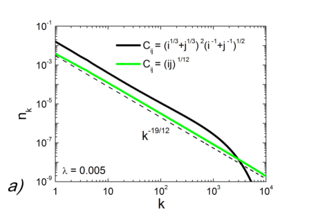
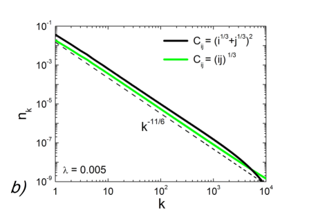
Figure 1: Particle size distribution in the case of complete decomposition into monomers. (a) The limiting case of energy equipartition $\left<E_{k}\right>={\rm const}$ for all species. The solid black line corresponds to the system with complete kinetic coefficients (9), while the solid green line corresponds to the simplified coefficients (12) with the same degree of homogeneity, $2\mu=1/6$. The dashed line has slope $n_{k}\propto k^{-19/12}$, predicted by the theory. (b) The limiting case of equal velocity dispersion for all species, $\left<{\bf v}_{k}^{2}\right>={\rm const}$. The solid black line refers to the system with the complete kinetic coefficients (11), while the solid green line corresponds to the simplified coefficients (12) with the same degree of homogeneity, $2\mu=2/3$. The dashed line shows the theoretical dependence, $n_{k}\propto k^{-11/6}$. In all cases the power-law distribution turns into an exponential decay for large sizes.

Our analytical findings are confirmed by simulations. In Fig. 1, the results of a direct numerical solution of the system of rate equations (3)–(2.2) are shown for both limiting kernels, (9) and (11), together with their simplified counterparts (12). The stationary distributions for the systems with the complete kinetic coefficients (9)–(11) have exactly the same slope as the systems with the simplified kernel (12) of the same degree of homogeneity and hence quantitatively agree with the theoretical prediction (15). Moreover, the numerical solutions demonstrate an exponential cutoff for large $k$, in agreement with the theoretical predictions.

Kernels (9) and (11) with homogeneity degree $\varkappa=1/6$ and $\varkappa=2/3$ correspond to two limiting cases of the size dependence of the average kinetic energy $\left<E_{k}\right>=\frac{1}{2}m_{k}\left<{\bf v}_{k}^{2}\right>\sim k^{\beta}$. Namely, $\beta=0$ corresponds to $\varkappa=1/6$ and $\beta=1$ to $\varkappa=2/3$. Physically, we expect that $\beta$ is constrained within the interval $0\leq\beta\leq 1$. Indeed, negative $\beta$ would imply vanishing velocity dispersion for very large particles, which is only possible for the unrealistic condition of the collision-free motion. The condition $\beta>1$ is unrealistic as well, since it would imply that the energy in the random motion, pumped by particle collisions, increases with particle mass faster than linearly; there is no evidence for such processes. We conclude that $\beta$ must be limited within the interval $[0,1]$, and therefore $\mu=\varkappa/2$ varies in the interval $1/12\leq\mu\leq 1/3$.

2.3 Power-law collisional decomposition and erosion

Although the fragmentation model with a complete decomposition into monomers allows a simple analytical treatment, a more realistic model implies power-law size distribution of debris [30, 31]; moreover, collisions with erosion also take place [31, 37].

Power-law decomposition. Experiments [30, 31] show that the number of debris particles of size $k$ produced in the fragmentation of a particle of size $i$ scales as $x_{k}(i)\sim B(i)/k^{\alpha}$. If the distribution $x_{k}(i)$ of the debris size is steep enough, the emerging steady-state particle distribution should be close to that for complete fragmentation into monomers. A scaling analysis, outlined below confirms this expectation, provided that $\alpha>2$; moreover, in this case $B(i)=i$ (see SI Appendix).

Substituting the debris size distribution $x_{k}(i)\sim i/k^{\alpha}$ into the basic kinetic equations (2.1), we notice that the equation for the monomer production rate coincides with Eq. (2.2), up to a factor in the coefficients $A_{ij}$. At the same time, the general equations (2.1) for $n_{k}$ have the same terms as Eqs. (3) for complete decomposition, but with two extra terms – the forth and fifth terms in Eqs. (2.1). These terms describe an additional gain of particles of size $k$ due to decomposition of larger aggregates. Assuming that the steady-state distribution has the same form as for monomer decomposition, $n_{k}\sim k^{-\gamma}e^{-\nu k}$, one can estimate (up to a factor) these extra terms for the homogeneous kinetic coefficients, $A_{ij}=\lambda C_{ij}\sim(ij)^{\mu}$ [see Eq. (12)]. One gets

$$\sum_{i=1}^{k}\sum_{j=k+1}^{\infty}A_{ij}n_{i}n_{j}B(j)k^{-\alpha}\sim k^{-\alpha}$$ (16)

$$\sum_{i,j\geq k}A_{ij}n_{i}n_{j}\left[B(i)+B(j)\right]k^{-\alpha}\sim k^{\mu-\gamma+1-\alpha}\,.$$ (17)

Here we also require that $\nu k\ll 1$, which is the region where the size distribution exhibits a power-law behavior. The above terms are to be compared with the other three terms in Eqs. (2.1) or Eqs. (3), which are the same for monomer and power-law decomposition:

$$\sum_{i+j=k}C_{ij}n_{i}n_{j}\sim\sum_{i\geq 1}C_{ik}n_{i}n_{k}\sim\sum_{i\geq 1}A_{ik}n_{i}n_{k}\sim k^{\mu-\gamma}\,.$$ (18)

If the additional terms (16) and (17) were negligible, as compared to the terms (18) that arise for both models, the emergent steady-state size distributions would be the same. For $k\gg 1$, one can neglect (16) and (17) compared to (18) if $\alpha>\gamma-\mu$ and $\alpha>1$. Taking into account that the equations for the monomers for the two models coincide when $\alpha>2$, we arrive at the following criterion for universality of the steady-state distribution: $\alpha>{\rm max}\left\{\gamma-\mu,2\right\}$. In the case of complete decomposition into monomers we have $\gamma=\mu+3/2$ [see (15)]. Hence the above criterion becomes $\alpha>2$. In other words, if $\alpha>2$, the model of complete decomposition into monomers yields the same steady-state size distribution as the model with any power-law distribution of debris.

Collisions with erosion. In collisions with erosion only a small fraction of a particle mass is chipped off [31, 37, 38]. Here we consider a simplified model of such collisions: It takes place when the relative kinetic energy exceeds the threshold energy $E_{\rm eros}$, which is smaller than the fragmentation energy $E_{\rm frag}$. Also, we assume that the chipped-off piece always contains $l$ monomers. Following the same steps as before one can derive rate equations that describe both disruptive and erosive collision. For instance, for complete decomposition into monomers the equation for $n_{k}$ with $k\geq l+2$ acquires two additional terms

$$\lambda_{e}\sum_{i=1}^{\infty}C_{i\,k+l}n_{i}n_{k+l}-\lambda_{e}\sum_{i=1}^{\infty}C_{ik}n_{i}n_{k},$$

with similar additional terms for $l+2>k>1$ and for the monomer equation. Here $\lambda_{e}$ gives the ratio of the frequencies of aggregative and erosive collisions, which may be expressed in terms of $E_{\rm eros}$ (see SI Appendix). We assume that $\lambda_{e}$ is small and is of the same order of magnitude as $\lambda$. We also assume that $\lambda_{e}$ is constant and that $l\lambda_{e}\ll 1$. Then we can shown that for $k\gg 1$ the size distribution of aggregates $n_{k}$ has exactly the same form, Eq. (15), as for the case of purely disruptive collisions (see SI Appendix).

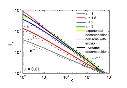
Figure 2: Particle size distribution in the case of power-law decomposition. The black solid line depicts the particle size distribution for the case of complete decomposition. The other solid lines show the emergent steady-state distributions for the following size distributions of debris: the power-law distribution, $x_{k}(i)\sim k^{-\alpha}$, with $\alpha=1$ (gray), $\alpha=1.5$ (red), $\alpha=2$ (blue), $\alpha=3$ (green), exponential distribution $x_{k}(i)\sim\exp\left(-k\right)$ (yellow) and collisions with an erosion, $\lambda_{e}=0.05$, $l=3$ (violet). The dashed lines indicate the corresponding fit $n_{k}\sim k^{-\gamma}$. Note that for steep size distributions of debris (power law with $\alpha>2$, exponential distribution) all slopes coincide with the one for the case of complete decomposition into monomers. All curves correspond to the case of constant kinetic coefficients with $\lambda=C_{ij}/A_{ij}=0.01$.

Universality of the steady-state distribution. The steady-state size-distribution of aggregates (15) is generally universal: It is the same for all size distributions of debris, with a strong dominance of small fragments, independently of its functional form. Moreover, it may be shown analytically (see SI Appendix), that the form (15) of the distribution persists when collisions with erosion are involved. We checked this conclusion numerically, solving the kinetic equations (2.1) with a power-law, exponential size distribution of debris and for collisions with an erosion (Fig. 2). We find that the particle size distribution (15) is indeed universal for steep distributions of debris size. Fig. 2 also confirms the condition of universality of the distribution (15), if $\alpha>2$ for power-law debris size-distributions.

A steep distribution of debris size, with strong domination of small fragments appears plausible from a physical point of view: The aggregates are relatively loose objects, with a low average coordination number, that is, with a small number of bonds between neighboring constituents; it is easy to break such objects into small pieces. The erosion at collision also has no qualitative impact on the size distribution as long as the frequency of such collisions is significantly less than of the aggregative ones.

2.4 Size distribution of the ring particles

The distribution of the ring particles’ radii, $F(R)$, is constrained by space- and earth-bound observations [16]. To extract $F(R)$ we use the relation $R^{3}=r_{k}^{3}=kr_{1}^{3}$ (for spherical particles) in conjunction with $n_{k}dk=F(R)dR$. We find that $n_{k}\sim k^{-3/2-\mu}\exp(-\lambda^{2}k)$ implies

$$F(R) \sim R^{-q}e^{-(R/R_{c})^{3}}\qquad q=5/2+3\mu$$ (19)

$$R_{c} = r_{1}/\lambda^{2/3}\,.$$ (20)

Thus for $R\ll R_{c}$ the distribution is algebraic with exponent $q=5/2+3\mu$, and the crossover to exponential behavior occurs at $R\sim R_{c}$.

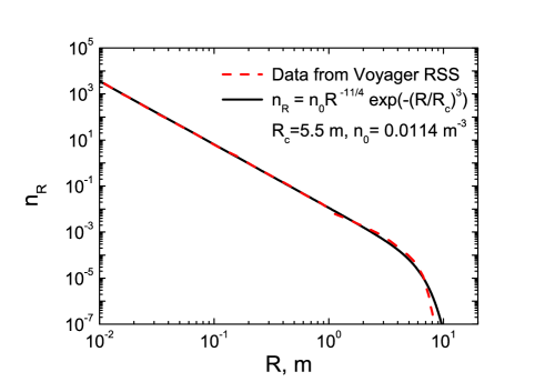
Figure 3: Particle size distribution for Saturn’s A ring. The dashed line represents the particle size distribution of Saturn’s A ring inferred from data obtained by the Voyager Radio Science Subsystem (RSS) during a radio occultation of the spacecraft by the rings [15]. A fit of the theoretical curve, Eq.(19), is shown as a solid line, giving a cutoff radius of $R_{c}=5.5\,{\rm m}$

We have shown that the exponent $\mu$ can vary within the interval $1/12\leq\mu\leq 1/3$, and hence the exponent $q$ for the size distribution varies in the range $2.75\leq q\leq 3.5$. This is in excellent agreement with observations, where values for $q$ in the range from $2.70$ to $3.11$ were reported [15, 17]. Fitting the theory to the particle size distribution of Saturn’s A ring inferred from data obtained by the Voyager Radio Science Subsystem (RSS) during a radio occultation of the spacecraft by Saturn’s A ring [15], we find $R_{c}=5.5$m (Fig. 3). For $r_{1}$ in the plausible range from $1$cm to $10$cm [16] we get (Eq. 20) $\lambda$ on the order of $10^{-4}$ to $10^{-3}$, which is the ratio of the frequencies of disruptive and coagulating collisions. It is also possible to estimate characteristic energies and the strength of the aggregates. Using the plausible range for random velocity, $v_{0}=0.01-0.1{\rm cm/s}$ [16], we obtain values that agree with the laboratory measurements (see SI Appendix).

3 Conclusion and Outlook

We have developed a kinetic model for the particle size distribution in a dense planetary ring and showed that the steady-state distribution emerges from the dynamic balance between aggregation and fragmentation processes. The model quantitatively explains properties of the particle size distribution of Saturn’s rings inferred from observations. It naturally leads to a power-law size distribution with an exponential cutoff (Eq. 19). Interestingly, the exponent $q=2.5+3\mu$ is universal, for a specific class of models we have investigated in detail. That is, $q$ does not depend on details of the collisional fragmentation mechanism, provided the size distribution of debris, emerging in an impact, is steep enough; collisions with erosion do not alter $q$ as well. The exponent $q$ is a sum of two parts: The main part, $2.5$, corresponds to the ”basic” case when the collision frequency does not depend on particle size ($\mu=0$); such slope is generic for a steady size-distribution, stemming from the aggregation-fragmentation balance in binary collisions. The additional part, $3\mu$, varying in the interval $0.25\leq 3\mu\leq 1$, characterizes size dependence of the collision frequency. The latter is determined by the particles’ diameters and the mean square velocities $\left<{\bf v}_{k}^{2}\right>$ of their random motion. We have obtained analytical solutions for the limiting cases of energy equipartition, $\frac{1}{2}m_{k}\left<{\bf v}_{k}^{2}\right>={\rm const}$, ($3\mu=0.25$) and of equal velocity dispersion for all species $\left<{\bf v}_{k}^{2}\right>={\rm const}$, ($3\mu=1$). These give the limiting slopes of $q=2.75$ and $q=3.5$. Physically, we expect that an intermediate dependence between these two limiting cases may follow from a better understanding of the behaviors of threshold energies. This would imply a power-law size distribution with exponent in the range $2.75\leq q\leq 3.5$.

Observed variations of spectral properties of ring particles [39, 40] may indicate differences in the surface properties, and thus, in their elasticity and sticking efficiency. This implies differences in the velocity dispersion $\left<{\bf v}_{k}^{2}\right>$ and its dependence on $k$, resulting in different values of the exponent $q$. Moreover, variations in particle sizes among different parts of Saturn’s ring system have been inferred from Cassini data [16, 41]. For our model, a different average particle size, or monomer size, implies different values of $E_{\rm frag}$ and $E_{\rm agg}$ as well as different values of the upper cutoff radius $R_{c}$. The model gives $R_{c}$ in terms of the primary grain radius and the ratio of the disruptive and aggregative collisions, Eq. (20). Since this ratio increases with increasing kinetic energy of particles’ random motion, the cutoff radius is expected to be smaller for rings with larger velocity dispersion.

Our results essentially depend on three basic assumptions: (i) ring particles are aggregates comprised from primary grains which are kept together by adhesive (or gravitational) forces; (ii) the aggregate sizes change due to binary collisions, which are aggregative, bouncing, or disruptive (including collisions with erosion); (iii) the collision rates and type of impacts are determined by sizes and velocities of colliding particles. We wish to stress that the power-law distribution with a cutoff is a direct mathematical consequence of the above assumptions only, that is, there is no need to suppose a power-law distribution and search for an additional mechanism for a cutoff as in previous semi-quantitative approaches [9].

The agreement between observations and predictions of our model for the size distribution indicates that dense planetary rings are indeed mainly composed of aggregates similar to the Dynamic Ephemeral Bodies suggested three decades ago [6, 7]. This means that the (ice) aggregates constituting the cosmic disks permanently change their mass due to collision-caused aggregation and fragmentation, while their distribution of sizes remains stationary. Thus, our results provide another (quantitative) proof that the particle size distribution of Saturn’s rings is not primordial. The same size distributions are expected for other collision dominated rings, as the rings of Uranus [42, 43], Chariklo [44, 45] and Chiron [46, 47], and possibly around extrasolar objects [48, 49, 50].

The predictive power of the kinetic model further emphasizes the role of adhesive contact forces between constituents which dominate for aggregate sizes up to the observed cutoff radius of $R_{c}\sim 5-10\,{\rm m}$. The model does not describe the largest constituents in the rings, with sizes beyond $R_{c}$. These are the propeller-moonlets in the A and B rings of Saturn, which may be remnants of a catastrophic disruption [20, 12]. We also do not discuss the nature of the smallest constituents, that is, of the primary grains. These particles are probably themselves comprised of still smaller entities and correspond to the least-size free particles observed in the rings [13].

Recently, cohesion was studied for dense planetary rings in terms of N-Body simulations [51, 52]. This model is similar to ours in that the authors use critical velocities for merging and fragmentation while we use threshold energies $E_{\rm agg}$ and $E_{\rm frag}$; both criteria are based on the cohesion model. In these simulations a power-law distribution for the aggregates size $F(R)\sim R^{-q}$ was obtained with slopes $2.75\leq q\leq 3$ for reasonable values of the cohesive parameter, consistent with our theoretical result. Moreover, the critical velocities for merging and fragmentation differ in most of the simulations by a factor of two, which is in reasonable agreement with our model, where we estimated $E_{\rm frag}$ to be roughly twice $E_{\rm agg}$ (SI Appendix). However, the simulations cannot resolve an exponential cutoff of $F(R)$, due to the small number of large aggregates, but the dependence of the largest aggregate size is inferred for different cohesion parameters and critical velocities.

4 Materials and Methods

4.1 Boltzmann equation

The general equations (2.1) for the concentrations $n_{k}$ have been derived from the Boltzmann kinetic equation. Here we consider a simplified case of a force-free and spatially uniform system. It is possible to take into account the effects of non-homogeneity, as it is observed in self-gravity wakes, and gravitational interactions between particles. These, however, do not alter the form of resulting rate equations (2.1), which may be then formulated for the space-averaged values (see SI Appendix).

Let $f_{i}\equiv f(m_{i},{\bf v}_{i},t)$ be the mass-velocity distribution function which gives density of particles of mass $m_{i}$ with the velocity ${\bf v}_{i}$ at time $t$. In the homogeneous setting, the distribution function evolves according to the Boltzmann equation,

$$\frac{\partial}{\partial t}f_{k}\left({\bf v}_{k},t\right)=I^{\rm b}_{k}+I^{\rm heat}_{k}+I^{\rm agg}_{k}+I^{\rm frag}_{k}\,,$$ (21)

where the right-hand side accounts for particles collisions. The first term $I^{\rm b}_{k}$ accounts for bouncing collisions of particles (see e.g. [24]), the second term $I^{\rm heat}_{k}$ describes the viscous heating caused by the Keplerian shear (see e.g. [53]); the terms $I^{\rm agg}_{k}$ and $I^{\rm frag}_{k}$ account, respectively, for the aggregative and disruptive impacts (explicit expressions for these terms are given in SI Appendix). To derive the rate equations (2.1) for the concentrations of the species, $n_{k}(t)=\int d{\bf v}_{k}f_{k}({\bf v}_{k},t)$, one needs to integrate Eq. (21) over ${\bf v}_{k}$. Assuming that all species have a Maxwell velocity distribution function with average velocity $\left<{\bf v}_{k}\right>=0$ and velocity dispersion $\left<{\bf v}_{k}^{2}\right>$ we obtain the rate equations (2.1) and the rate coefficients (2.1) (see SI Appendix for the detail).

4.2 Generating Function Techniques

To solve Eqs. (6) we use the generating function $\mathcal{N}(z)=\sum_{k\geq 1}n_{k}\,z^{k}$ which allows us to convert these equations into the single algebraic equation

$$\mathcal{N}(z)^{2}-2(1+\lambda)N\mathcal{N}(z)+2(1+\lambda)Nn_{1}z=0\,.$$ (22)

Its solution reads

$$\mathcal{N}(z)=\left(1+\lambda\right)N\left[1-\sqrt{1-\frac{2n_{1}}{(1+\lambda)N}\,z}\,\right]\,.$$ (23)

Expanding $\mathcal{N}(z)$ we arrive at the distribution (7).

4.3 Efficient numerical algorithm

  The numerical solution of Smoluchowski-type equations (2.1) is challenging as one has to solve infinitely many coupled non-linear equations. We developed an efficient and fast numerical algorithm dealing with a large number of such equations. The application of our algorithm requires the condition

$$\sum_{i=1}^{k}C_{i,k+1}n_{i}\gg\sum_{i=k+1}^{N}C_{i,k+1}n_{i}$$ (24)

is obeyed for $k\gg 1$ and $N\gg 1$, where $n_{i}$ are the steady-state concentrations. For the case of interest this condition is fulfilled. Our algorithm first solves a relatively small set ($\sim 100$) of equations using the standard technique and then obtains other concentrations of much larger set ($\sim 10,000$) using an iterative procedure (see SI Appendix).

- [1] Cuzzi, J. N. & Durisen, R. H. Bombardment of planetary rings by meteoroids - General formulation and effects of Oort Cloud projectiles. Icarus 84, 467–501 (1990).
- [2] Cuzzi, J. N. & Estrada, P. R. Compositional Evolution of Saturn’s Rings Due to Meteoroid Bombardment. Icarus 132, 1–35 (1998).
- [3] Tiscareno, M. S. et al. Observations of Ejecta Clouds Produced by Impacts onto Saturn’s Rings. Science 340, 460–464 (2013).
- [4] Cuzzi, J. et al. An Evolving View of Saturn’s Dynamic Rings. Science 327, 1470–1475 (2010).
- [5] Harris, A. W. Collisional breakup of particles in a planetary ring. Icarus 24, 190–192 (1975).
- [6] Davis, D. R., Weidenschilling, S. J., Chapman, C. R. & Greenberg, R. Saturn ring particles as dynamic ephemeral bodies. Science 224, 744–747 (1984).
- [7] Weidenschilling, S. J., Chapman, C. R., Davis, D. R. & Greenberg, R. Ring particles - Collisional interactions and physical nature. In Planetary Rings, 367–415 (1984).
- [8] Gorkavyi, N. & Fridman, A. M. Astronomy Letters 11, 628 (1985).
- [9] Longaretti, P. Y. Saturn’s main ring particle size distribution: An analytic approach. Icarus 81, 51–73 (1989).
- [10] Canup, R. M. & Esposito, L. W. Accretion in the Roche zone: Coexistence of rings and ring moons. Icarus 113, 331–352 (1995).
- [11] Spahn, F., Albers, N., Sremcevic, M. & Thornton, C. Kinetic description of coagulation and fragmentation in dilute granular particle ensembles. Europhysics Letters 67, 545–551 (2004).
- [12] Esposito, L. Planetary Rings (2006).
- [13] Bodrova, A., Schmidt, J., Spahn, F. & Brilliantov, N. Adhesion and collisional release of particles in dense planetary rings 218, 60–68 (2012).
- [14] Marouf, E. A., Tyler, G. L., Zebker, H. A., Simpson, R. A. & Eshleman, V. R. Particle size distributions in Saturn’s rings from Voyager 1 radio occultation. Icarus 54, 189–211 (1983).
- [15] Zebker, H. A., Marouf, E. A. & Tyler, G. L. Saturn’s rings - Particle size distributions for thin layer model. Icarus 64, 531–548 (1985).
- [16] Cuzzi, J. et al. Ring Particle Composition and Size Distribution, 459–509 (Springer, 2009).
- [17] French, R. G. & Nicholson, P. D. Saturn’s Rings II. Particle sizes inferred from stellar occultation data. Icarus 145, 502–523 (2000).
- [18] Zebker, H. A., Tyler, G. L. & Marouf, E. A. On obtaining the forward phase functions of Saturn ring features from radio occultation observations. Icarus 56, 209–228 (1983).
- [19] Tiscareno, M. S. et al. 100-metre-diameter moonlets in Saturn’s A ring from observations of ’propeller’ structures. Nature 440, 648–650 (2006).
- [20] Sremcevic, M. et al. A Belt of Moonlets in Saturn’s A ring. Nature 449, 1019–1021 (2007).
- [21] Tiscareno, M. S., Burns, J. A., Hedman, M. M. & Porco, C. C. The Population of Propellers in Saturn’s A Ring. The Astronomical Journal 135, 1083–1091 (2008).
- [22] Guimaraes, A. H. F. et al. Aggregates in the strength and gravity regime: Particles sizes in saturn’s rings. Icarus 220, 660–678 (2012).
- [23] Borderies, N., Goldreich, P. & Tremaine, S. A granular flow model for dense planetary rings. Icarus 63, 406–420 (1985).
- [24] Brilliantov, N. V. & Pöschel, T. Kinetic Theory of Granular Gases (Oxford University Press, Oxford, 2004).
- [25] Araki, S. & Tremaine, S. The dynamics of dense particle disks. Icarus 65, 83–109 (1986).
- [26] Araki, S. The dynamics of particle disks. II. Effects of spin degrees of freedom. Icarus 76, 182–198 (1988).
- [27] Araki, S. The dynamics of particle disks III. Dense and spinning particle disks. Icarus 90, 139–171 (1991).
- [28] Dominik, C. & Tielens, A. G. G. The Physics of Dust Coagulation and the Structure of Dust Aggregates in Space. Astrophys. J. 480, 647 (1997).
- [29] Wada, K. Collisional Growth Conditions for Dust Aggregates. Astrophys. J. 702, 1490–1501 (2009).
- [30] Astrom, J. A. Statistical models of brittle fragmentation. Advances in Physics 55, 247–278 (2006).
- [31] Guettler, C., Blum, J., Zsom, A., Ormel, C. & Dullemond, C. P. The outcome of protoplanetary dust growth: pebbles, boulders, or planetesimals? 1. mapping the zoo of laboratory collision experiments. Astronomy and Astrophysics, A 56, 513 (2010).
- [32] Srivastava, R. C. J. Atom. Sci. 39, 1317 (1982).
- [33] Salo, H. Numerical simulations of dense collisional systems: II. Extended distribution of particle size. Icarus 96, 85–106 (1992).
- [34] Bodrova, A., Levchenko, D. & Brilliantov, N. Universality of temperature distribution in granular gas mixtures with a steep particle size distribution. Europhysics Letters 106, 14001 (2014).
- [35] Leyvraz, F. Scaling theory and exactly solved models in the kinetics of irreversible aggregation. Physics Reports 383, 95–212 (2003).
- [36] Krapivsky, P. L., Redner, A. & Ben-Naim, E. A Kinetic View of Statistical Physics (Cambridge University Press, Cambridge, UK, 2010).
- [37] Schrapler, R. & Blum, J. The physics of protopanetesimal dust agglomerates. vi. erosion of large aggregates as a source of micrometer-sized particles. Astrophys. J. 734, 108 (2011).
- [38] Krapivsky, P. L. & Ben-Naim, E. Shattering transitions in collision-induced fragmentation. Phys. Rev. E 68, 021102 (2003).
- [39] Nicholson, P. D. et al. A close look at Saturn’s rings with Cassini VIMS. Icarus 193, 182–212 (2008).
- [40] Filacchione, G. et al. Saturn’s icy satellites and rings investigated by Cassini-VIMS. III. Radial compositional variability. Icarus (2012).
- [41] Colwell, J. E., Cooney, J., Esposito, L. W. & Sremcevic, M. Saturn’s Rings Particle and Clump Sizes from Cassini UVIS Occultation Statistics. AGU Fall Meeting Abstracts 1 (2013).
- [42] Elliot, J. L. & Nicholson, P. D. The rings of uranus. In Planetary Rings, 25–72 (1984).
- [43] Elliot, J. L., French, R. G., Meech, K. J. & Elias, J. H. Structure of the Uranian rings. I - Square-well model and particle-size constraints. Astron. J. 89, 1587–1603 (1984).
- [44] Braga-Ribas, F. et al. A ring system detected around the Centaur(10199) Chariklo. Nature 1–13 (2014).
- [45] Duffard, R. et al. Photometric and spectroscopic evidence for a dense ring system around Centaur Chariklo. A&A 568, A79 (2014).
- [46] Ortiz, J. L. et al. Possible ring material around centaur (2060) Chiron. A&A 576, A18 (2015).
- [47] Ruprecht, J. D. et al. 29 November 2011 stellar occultation by 2060 Chiron: Symmetric jet-like features. Icarus 252, 271–276 (2015).
- [48] Ohta, Y., Taruya, A. & Suto, Y. Predicting Photometric and Spectroscopic Signatures of Rings Around Transiting Extrasolar Planets. ApJ 690, 1–12 (2009).
- [49] Mamajek, E. E. et al. Planetary Construction Zones in Occultation: Discovery of an Extrasolar Ring System Transiting a Young Sun-like Star and Future Prospects for Detecting Eclipses by Circumsecondary and Circumplanetary Disks. The Astronomical Journal 143, 72 (2012).
- [50] Kenworthy, M. A. et al. Mass and period limits on the ringed companion transiting the young star J1407. Monthly Notices RAS 446, 411–427 (2015).
- [51] R. P. Perrine, D. C. Richardson and D. J. Scheeres. A numerical model of cohesion in planetary rings. Icarus 212, 719735 (2011).
- [52] R. P. Perrine and D. C. Richardson. N-body simulations of cohesion in dense planetary rings: A study of cohesion parameters. Icarus 219, 515533 (2012).
- [53] Schmidt, J., Ohtsuki, K., Rappaport, N., Salo, H. & Spahn, F. Dynamics of Saturn’s Dense Rings, 413–458 (Springer, 2009).
- [54] Garzo, V. & Dufty, J. W. Phys. Rev. E 59, 5895 (1999).
- [55] Brilliantov, N. V. & Spahn, F. Mathematics and Computers in Simulation 72, 93 (2006).
- [56] Garzo, V., Hrenya, C. M. & Dufty, J. W. Enskog theory for polydisperse granular mixtures. ii. sonine polynomial approximation. Phys. Rev. E 76, 031304 (2007).
- [57] Piasecki, J., Trizac, E. & Droz, M. Dynamics of ballistic annihilation. Phys. Rev. E 66, 066111 (2002).
- [58] Colwell, J. E. et al. The Structure of Saturn’s Rings, 375 (Springer, 2009).
- [59] Salo, H. Gravitational wakes in Saturn’s rings. Nature 359, 619–621 (1992).
- [60] Colwell, J. E., Esposito, L. W. & Sremcevic, M. Self-gravity wakes in saturn’s a ring measured by stellar occultations from cassini. Geophysical Research Letters 33, L07201 (2006).
- [61] Hedman, M. et al. Self-gravity wake structures in saturn’s a ring revealed by cassini vims. Astronomical Journal 133, 2624–2629 (2007).
- [62] French, R. G., Salo, H., McGhee, C. A. & Dones, L. H. Hst observations of azimuthal asymmetry in saturn’s rings. Icarus 189, 493–522 (2007).
- [63] Toomre, A. On the gravitational stability of a disk of stars. Astrophys. J. 139, 1217–1238 (1964).
- [64] Résibois, P. & De Leener, M. Classical kinetic theory of fluids (Wiley & Sons, New York, 1977).
- [65] Peters, E. A., Kollmann, M., Barenbrug, T. M. & Philipse, A. P. Caging of a d-dimensional sphere and its relevance for the random dense sphere packing. Phys. Rev. E 63, 021404 (2001).
- [66] A.P. Hatzes, D. N. C. L., F. Bridges & Sachtjen, S. Coagulation of Particles in Saturn’s Rings: Measurements of the Cohesive Force of Water Frost. Icarus 89, 113–121 (1991).
- [67] F. Bridges, D. N. C. L. R. K., K. D. Supulver & Zafra, M. Energy Loss and Sticking Mechanisms in Particle Aggregation in Planetesimal Formation. Icarus 123, 422435 (1996).
- [68] Brilliantov, N. V., Albers, N., Spahn, F. & Pöschel, T. Collision dynamics of granular particles with adhesion. Phys. Rev. E 76, 051302 (2007).
- [69] Flajolet, P. & Sedgewick, R. Analytic Combinatorics (Cambridge University Press, 2009).