Structure of CB 26 Protoplanetary Disk Derived from Millimeter Dust Continuum Maps

Abstract

Observations of the circumstellar disk in the Bok globule CB 26 at 110, 230, and 270 GHz are presented together with the results of the simulations and estimates of the disk parameters. These observations were obtained using the SMA, IRAM Plateau de Bure, and OVRO interferometers. The maps have relatively high angular resolutions (0.4 – 1^′′), making it possible to study the spatial structure of the gas–dust disk. The disk parameters are reconstructed via a quantitative comparison of observational and theoretical intensity maps. The disk model used to construct the theoretical maps is based on the assumption of hydrostatic and radiative equilibrium in the vertical direction, while the radial surface density profile is described phenomenologically. The system of equations for the transfer of the infrared and ultraviolet radiation is solved in the vertical direction, in order to compute the thermal structure of the disk. The disk best-fit parameters are derived for each map and all the maps simultaneously, using a conjugate gradient method. The degrees of degeneracy of the parameters describing the thermal structure and density distribution of the disk are analyzed in detail. All three maps indicate the presence of an inner dust-free region with a radius of approximately 35 AU, in agreement with the conclusions of other studies. The inclination of the disk is 78^∘, which is smaller than the value adopted in our earlier study of rotating molecular outflows from CB 26. The model does not provide any evidence for the growth of dust particles above $a_{\rm max}\approx 0.02$ cm.

1 Introduction

The rapidly growing number of detected planetary systems, which have very different orbital configurations and orbit stars with masses varying over a wide range, suggests that the formation of planets is a widespread process in the Galaxy. Since gas–dust disks are natural predecessors of planetary systems, theoretical and observational studies of such disks have become intense over the past decade.

According to current understanding, stars are formed during the gravitational collapse of molecular clouds McKee and Ostriker (2007). Since clouds always have non-zero angular momenta, the collapsing matter cannot directly fall into a protostar, and fairly rapidly (over $\sim 10^{4}$ yr) forms a circumstellar disk surrounded by an envelope Hueso and Guillot (2005). The angular momentum inside the disk is redistributed so that the bulk of the matter falls onto the protostar, and only a smaller portion moves outward, carrying away angular momentum Lynden-Bell and Pringle (1974); Armitage (2011); Tutukov and Pavlyuchenkov (2004). The characteristic evolutionary timescales of dust disks around young single stars are several million years Haisch et al. (2001). At this time, a key mechanism is initiated that can eventually lead to the formation of planets: the growth of the size of the dust particles and their settling toward the central plane of the disk. The enlargement of dust particles with the subsequent formation of planetesimals form the basis of the core accretion theory Safronov (1969), which appears to describe the main regime of planetary formation Janson et al. (2012). The evolution of dust in disks around young stars is confirmed by their observed spectral energy distributions (SEDs) in the IR and (sub)millimeter McClure et al. (2010); Andrews and Williams (2005); together with the high rate of occurence of exoplanets, this suggests a protoplanetary nature for these disks. Additional important factors affecting the evolution of young stars are bipolar jets, outflows, and disk winds Pudritz et al. (2007), which play an important role in the final stages of evaporation of the gaseous disk. The variety of controlling processes and the wide range of their physical parameters makes protoplanetary disks very interesting objects; a complete understanding of their nature will be only possible through a synthesis of modern observations and detailed simulations.

Observations of protoplanetary disks are difficult, since these objects have relatively small sizes and low temperatures, but a number of basic facts concerning their evolution and structures have been more or less reliably established Williams and Cieza (2011). Observations in the middle-IR can be used to determine the rate of occurence and lifetime of these disks Mamajek (2009). Their masses can be determined using millimeter observations Mann and Williams (2010), and the structures of protoplanetary disks can be reconstructed using interferometric observations Sauter and Wolf (2011). A number of tools have been developed as a theoretical basis for understanding the physics of protoplanetary disks, and for the interpretation of SEDs (see, e.g., the list of publicly available software codes in Wood (2008)). However, the problem of degeneracy remains, when observations are equally well described by several sets of parameters, and a model can only provide limits for these sets Hetem and Gregorio-Hetem (2007). Increasing the angular resolution of observations can help to resolve this problem. Spatially resolved observations are currently available for more than one hundred and fifty protoplanetary disks at wavelengths from the optical to the radio, in both molecular lines and the continuum. These high-quality observational data require adequate interpretations and new approaches to deriving as much information as possible about the physical and chemical structure of the disk. The successful determination of the parameters of a number of protoplanetary disks using multi-frequency, spatially resolved observations Kwon et al. (2011); Madlener et al. (2012) and the operation of the ALMA interferometer make this area promising.

The aim of our study is to determine a self-consistent physical structure for the protoplanetary disk located at the edge of the Bok globule CB 26. This disk is about a hundred AU in size, has a mass of $0.1M_{\odot}$, and belongs to Class I of young stellar objects according to the classification of Lada (1987). The disk in CB 26 has been well studied and modeled Launhardt and Sargent (2001); Stecklum et al. (2004). A rotating outflow responsible for the removal of angular momentum from the disk was detected in Launhardt et al. (2009). A central region $45\pm 5$ AU in size where dust is depleted was later discovered in the disk using spatially resolved observations at 230 GHz Sauter et al. (2009). The best-fit model was derived by comparing observed images and synthetic maps. However, due to the computationally intensive method used for the radiative-transfer calculations, a step-by-step method was used to determine the parameters, and possible degeneracy of the model parameters was not analyzed. Another shortcoming of the above work is the phenomenological law used for the disk density distribution in the vertical direction. Our aim is to develop new tools to reconstruct disk structure and advanced routine to identify best-fit model parameters and their degeneracies. We aim to determine to what degree the modeling of mm maps of CB 26 are reproducible and reliable in the light of (a) new observations with the IRAM Plateau de Bure Interferometer (PdBI), (b) a refined model for the vertical density distribution, and (c) a more well-grounded parameter search technique.

The paper contains four sections, describing the observations, a physical model for the disk, the procedures used to obtain the synthetic maps, and our searches for the best-fit model. The main results and conclusions are given at the end of the paper.

2 OBSERVATIONS AND DATA REDUCTION

2.1 OVRO observations

CB 26 was observed with the Owens Valley Radio Observatory (OVRO) interferometer between January 2000 and December 2001. The 1.3 and 2.7 mm continuum emission was observed simultaneously in 2-GHz bands using an analog correlator, except in the highest-resolution configuration, where the 4-GHz capability of the new 1 mm receivers was used. Four configurations of the six 10.4 m antennas provided baselines in the range 10 – 170 k$\lambda$ at 2.7 mm (110 GHz) and 10 – 370 k$\lambda$ at 1.3 mm (236 GHz). The average system noise temperatures of the He-cooled SIS receivers were 300 – 400 K at 110 GHz and 300 – 600 K at 236 GHz. The observing parameters are summarized in Table 1.

Table 1: Millimeter interferometric observations of CB 26 in the continuum: $\lambda_{0}$ and $\nu_{0}$ are the central wavelength and frequency, $\theta$ the width of the antenna main beam, $a$ and $b$ the semi-major and semi-minor axes of the interferometer beam, PA the position angle of the beam major axis measured from the northern protoplanetary disk axis in the clockwise direction, $\sigma_{\nu}$ the rms map uncertainty in mJy/$\Omega_{\nu}$, and $\Omega_{\nu}=1.133ab$ the effective solid angle of the beam.

Telescope		$\lambda_{0}$	$\nu_{0}$	$\theta$	$a\times b$	PA	$\sigma_{\nu}$
					HPBW
		[mm]	[GHz]	[′′]	[′′]	[deg]	[mJy/$\Omega_{\nu}$]
OVRO	2001	2.7	110	65	$1.20\times 0.88$	93	0.3
PdBI	2005/08	3.4	88	57	$3.18\times 3.02$	102	0.1
OVRO	2001	1.3	236	25	$0.58\times 0.40$	92	0.6
PdBI	2005/09	1.3	230	22	$0.46\times 0.39$	22	0.3
SMA	2006	1.1	270	47	$1.00\times 0.84$	$-$89	2.7
OVRO+PdBIa)	2001–08	2.7	110	60	$1.37\times 1.05$	124	0.15
OVRO+PdBIa)	2001–09	1.3	230	22	$0.39\times 0.36$	75	0.5
SMAa)	2006	1.1	270	47	$1.00\times 0.84$	$-$57	2.7

a) Composite maps have been rotated by 32^∘ in order for the plane of the disk to align with the $x$ axis.

The amplitude and phase calibration were based on frequent observations of a nearby quasar. The flux densities were calibrated using observations of Uranus and Neptune, yielding relative uncertainties of 20%. The raw data were calibrated and edited using the MMA software package Scoville et al. (1993). The mapping and data analysis were carried out using the MIRIAD package Sault et al. (1995). The final maps were obtained by combining the OVRO and IRAM PdBI data.

2.2 IRAM PdBI observations

Observations of CB 26 were carried out with the IRAM Plateau de Bure Interferometer in November 2005 (D configuration with five antennas) and December 2005 (C configuration with six antennas; project PD0D). Two receivers were used simultaneously, tuned to single side bands at 89.2 GHz and 230.5 GHz, respectively. Higher resolution observations at 230 GHz were carried out in January 2009 (B configuration with six antennas) and February 2009 (A configuration with six antennas; Project S078). Further observations at 86.7 GHz were obtained in November 2008 (C configuration) and March 2009 (D configuration; project SC1C) with six antennas, using the new 3 mm receivers. Several nearby phase calibrators were observed during each track to determine the time-dependent complex antenna gains. The correlator bandpass was calibrated using 3C 454.3 and 3C 273, and the absolute flux-density scale was derived from observations of MWC 349. The flux calibration uncertainty is estimated to be $\leq$20% at both wavelengths. The observing parameters are summarized in Table 1.

The raw data were calibrated and imaged using the latest version of the GILDAS software. The final maps were obtained by combining the OVRO and PdBI data.

2.3 SMA Observations

Observations with the Submillimeter Array (SMA, Ho et al. (2004)) were made on December 6, 2006 (extended configuration) and December 31, 2006 (compact configuration), covering frequencies from 267 to 277 GHz in the lower and upper sidebands, respectively, and providing baselines of 12 – 62 k$\lambda$. The typical system temperatures were 350 – 500 K. The quasar 3C 279 was used for the bandpass calibration, and the quasars B0355+508 and 3C 111 for the gain calibration. Uranus was used for the absolute flux calibration, which is accurate to 20% – 30%. The 1.1 mm continuum map was constructed using line-free channels in both sidebands. The main observational parameters are summarized in Table 1. The raw data were calibrated using the IDL MIR package Qi (2005) and visualized using a package MIRIAD.

3 PHYSICAL MODEL

A global aim of this paper is to develop a set of software for determining the parameters of protoplanetary disks using observed millimeter maps. The reconstruction of the disk parameters is based on a quantitative comparison of synthetic and observed images of the disk. Mathematically, the problem is reduced to searching for the minimum of the parameter-dependent function describing the difference between the observed and synthetic maps. In this Section, we present the protoplanetary disk model used to construct the synthetic maps.

The main sources of disk heating in the model are the radiation of the central star and viscous heating (important only in dense central regions), while the source of cooling is thermal radiation in the continuum. Determining the disk’s thermal structure is reduced to the problem of radiative transfer in a dusty medium, since the dust contributes mostly to the opacity of the matter in protoplanetary disks. The density distribution in a low-mass disk around a single star can be considered to be axially symmetric in a first approximation (this is also valid for peripheral regions around close binaries). The thickness of the disk increases fairly rapidly with radius, so that the central star directly illuminates not only the inner edge of the disk, but also its peripheral parts Kenyon and Hartmann (1987). Moreover, the dust temperature is mainly determined by the radiation incident from the disk surface, i.e., by the vertical radiation transfer, since the optical depth rapidly increases in the radial direction. This makes it possible to decompose the two-dimensional problem and construct a so-called 1+1D model of the protoplanetary disk, in which the vertical and radial structures of the disk are determined independently D’Alessio et al. (1998); Dullemond et al. (2002).

The radial distribution of the surface density in our model is given by the analytical expression

$$\Sigma_{\rm T}=\Sigma_{0}^{\rm gas}\left(\frac{R}{1\,\mbox{AU}}\right)^{p},$$ (1)

whose parameters are determined from observational data. The disk was considered to be hydrostatic in the vertical direction, and the gas-density distribution was calculated based on its temperature. The dust and gas were assumed to be well mixed, so that the ratio of their densities did not change over the disk, and was equal to 0.01. It was additionally assumed that the gas and dust temperatures were equal; this equality is achieved in dense regions due to effective collisions between the dust particles and molecules. In the disk atmosphere, the gas can be much more hotter than the dust Jonkheid et al. (2004), but there is only a small mass of dust in this region. Therefore, the assumption that the dust and gas temperatures are equal is justified when obtaining synthetic maps of the disk in the mm, where the disk is optically thin and the radiation-intensity distribution reflects the dust density distribution.

The calculation of radiation transfer in a protoplanetary disk is a computationally intensive task due to the high optical depths for photons in the UV (up to $\sim 10^{5}$). Since the computation time required to calculate one model is critical to searches for the best-fit model, we developed a fast method for calculating the dust temperature in the disk with acceptable accuracy. This was achieved through an accurate transition to a two-frequency approximation and the use of the Schuster–Schwarzschild and Eddington approximations. We tested the method and compared it with another algorithm for calculating the radiative transfer, in which the dust opacity coefficients are functions of the wavelength. The transition from monochromatic opacities to mean opacities makes it possible to appreciably reduce the computational time without losing accuracy when calculating the dust temperature.

3.1 Momentum Equations for the IR Radiation Transfer

Let us consider a ring in the disk at the radius $R$. The gas surface density at this radius, in a layer between the equatorial plane and the surface of the disk, is $\Sigma_{\rm T}$. The key assumption of the model is that the disk does not radiate in the UV. Thus, we divided the spectral range into UV and IR parts and describe them separately. It was also assumed that the disk is geometrically thin and the plane-parallel approximation is valid. If $\Sigma=\int\limits_{0}^{z}\rho(\tilde{z})d\tilde{z}$ is the surface density in a layer from 0 to $z$, then the momentum equations for IR radiation transfer in the grey and Eddington approximations can be represented in the form

$$\dfrac{dF}{d\Sigma}=c\kappa_{P}(B-E),$$ (2)

$$F=-\dfrac{c}{3\kappa_{R}}\dfrac{dE}{d\Sigma},$$ (3)

where $F$ [erg cm^-2 s^-1] and $E$ [erg cm^-3] are the integrated energy flux and energy density, $B=aT^{4}$ is the integrated density of black-body radiation, and $\kappa_{P}$ and $\kappa_{R}$ [cm² g^-1] are the Planck and Rosseland mean opacities:

$$\kappa_{P}=\dfrac{\int\limits_{0}^{\infty}\kappa_{\nu}^{\rm abs}B_{\nu}d\nu}{\int\limits_{0}^{\infty}B_{\nu}d\nu},$$ (4)

$$\dfrac{1}{\kappa_{R}}=\dfrac{\int\limits_{0}^{\infty}\dfrac{1}{\left(\kappa_{\nu}^{\rm abs}+\kappa_{\nu}^{\rm sca}\right)}\dfrac{\partial B_{\nu}}{\partial T}d\nu}{\int\limits_{0}^{\infty}\dfrac{\partial B_{\nu}}{\partial T}d\nu}.$$ (5)

Here, $\kappa_{\nu}^{\rm abs}$ and $\kappa_{\nu}^{\rm sca}$ are the monochromatic coefficients of true absorption and scattering. Note that $\kappa_{P}$ and $\kappa_{R}$ are functions of the dust temperature.

3.2 Balance Equation and the Heating Functions

The equations considered must be closed by an energy-balance equation. The total radiative flux in the IR is due to heating of the surrounding medium. The change in this flux in the vertical direction is described by the formula

$$\frac{dF}{d\Sigma}=S_{\rm star}+S_{\rm acc}.$$ (6)

Here, $S_{\rm star}$ and $S_{\rm acc}$ [erg s^-1 g^-1] represent the heating due to stellar UV radiation and gas accretion. The stellar radiation heating function is

$$S_{\rm star}=4\pi\kappa_{P}^{\rm uv}J_{\rm uv},$$ (7)

where $\kappa_{P}^{\rm uv}$ is the Planck mean true absorption coefficient in the UV per unit mass, and $J_{\rm uv}$ is the UV intensity averaged over angles and frequencies. We used the two-flux Schuster–Schwarzschild approximation to calculate $J_{\rm uv}$, assuming that the disk does not radiate in the UV, and only absorbs and scatters the stellar radiation. The corresponding system of equations has the form

$$\dfrac{dF_{\rm uv}}{d\Sigma}=-4\pi\kappa_{P}^{\rm uv}J_{\rm uv},$$ (8)

$$F_{\rm uv}=-\dfrac{4\pi}{4\kappa_{F}^{\rm uv}}\dfrac{dJ_{\rm uv}}{d\Sigma},$$ (9)

where $\kappa_{F}^{\rm uv}$is the mean flux extinction coefficient (true absorption and scattering), and $F_{\rm uv}$ is the UV flux.

The boundary conditions at the surface of the disk can be written in the form

$$F_{\rm uv}=2\pi J_{\rm uv}-2\pi J_{\rm uv}^{-},$$ (10)

where $J_{\rm uv}^{-}$ is the intensity of the stellar radiation averaged over a hemisphere:

$$J_{\rm uv}^{-}=\dfrac{f}{\pi}\cdot L_{\rm star}/(4\pi R^{2}).$$ (11)

The coefficient $f$ determines the portion of the stellar radiation intercepted by the disk. Generally, $f$ depends on the inclination of the disk surface relative to the incident radiation. It is natural to combine the input model parameters $f$ and $L_{\rm star}$ into a single parameter $f\cdot L_{\rm star}$, representing the portion of the stellar luminosity intercepted by the disk.

The above system of equations can be solved analytically, if the opacities do not depend on $\Sigma$, or numerically, e.g., using the finite difference method. The UV opacities are defined as follows:

$$\kappa_{P}^{\rm uv}=\dfrac{\int\limits_{0}^{\infty}\kappa_{\nu}^{\rm abs}B_{\nu}d\nu}{\int\limits_{0}^{\infty}B_{\nu}d\nu},$$ (12)

$$\kappa_{F}^{\rm uv}=\dfrac{\int\limits_{0}^{\infty}\left(\kappa_{\nu}^{\rm abs}+\kappa_{\nu}^{\rm sca}\right)B_{\nu}d\nu}{\int\limits_{0}^{\infty}B_{\nu}d\nu}.$$ (13)

Here, the Planck function $B_{\nu}$ depends on the stellar temperature. Assuming that the gravitational energy release is proportional to the density, the heating function due to gas accretion is

$$S_{\rm acc}=\frac{G\dot{M}M_{\rm star}}{4\pi\Sigma_{\rm T}R^{3}},$$ (14)

where $\dot{M}$ is the accretion rate, and $M_{\rm star}$ is the stellar mass.

3.3 Solution of the System of Equations for the Thermal Structure

The above heating functions depend only on the surface density. Let us assume for the moment that $\kappa_{P}$ and $\kappa_{R}$ are only functions of the surface density (they are functions of temperature as well, but this problem will be solved further using an iteration process). In this case, we can obtain an analytical solution for $T(\Sigma)$. The temperature can be determined from Equations (2) and (6), i.e., from the relationship

$$c\kappa_{P}(aT^{4}-E)=S_{\rm star}+S_{\rm acc}.$$ (15)

It is necessary to find $E(\Sigma)$ in order to obtain $T(\Sigma)$. We integrate Equation (6) and obtain $F=F(\Sigma)$. Then, $F(\Sigma)$ is substituted in Equation (3), and the latter is integrated as $\int\limits_{0}^{\Sigma}d\Sigma^{\prime}$. As a result, we obtain an equation with the known function $\delta_{E}(\Sigma)$

$$E(\Sigma)-E(0)=\delta_{E}(\Sigma).$$ (16)

We must know the radiation energy density $E(0)$ in the equatorial plane of the disk in order to reconstruct $E(\Sigma)$ from this relationship. The radiation density can be found from boundary conditions. If the IR radiation from the disk is isotropic at the disk surface, i.e., at $\Sigma$=$\Sigma_{\rm T}$, whereas the IR radiation from the star can be neglected compared to the radiation from the disk itself, then $F(\Sigma_{0})=\dfrac{1}{2}cE(\Sigma_{\rm T})$. Therefore, the radiation energy density at the disk surface is

$$E(\Sigma_{\rm T})=\dfrac{2F(\Sigma_{\rm T})}{c}.$$ (17)

The formulas for $E(0)$ are obtained from (16) for $\Sigma=\Sigma_{\rm T}$:

$$E(0)=E(\Sigma_{\rm T})-\delta_{E}(\Sigma_{\rm T}).$$ (18)

When constructing the solution, we assumed that $\kappa_{P}$ and $\kappa_{R}$ are functions only of the surface density, not the temperature. An iterative process was implemented to solve this problem. After the thermal structure was found for the given opacities, we recalculated the opacities using information on the temperature profile $T(\Sigma)$. The new opacities were then used to recalculate a refined thermal structure. In practice, this iterative process converged over 8 – 10 steps.

3.4 Equation of Hydrostatic Equilibrium

The equation of hydrostatic equilibrium for a geometrically thin disk has the form

$$\dfrac{1}{\rho}\dfrac{d}{dz}(c_{T}^{2}\rho)=-\dfrac{GM_{\rm star}}{R^{3}}z,$$ (19)

where $c_{T}^{2}$is the sound speed. Since $T$, and therefore $c_{T}^{2}$ as a function of $\Sigma$, (but not as function of $z$) is known, the latter equation should be written in the form

$$\dfrac{dz}{d\Sigma}=\dfrac{1}{\rho},$$ (20)

$$\dfrac{d}{d\Sigma}(c_{T}^{2}\rho)=-\dfrac{GM_{\rm star}}{R^{3}}z.$$ (21)

This system of equations can be solved using the explicit integration scheme if the density $\rho(0)$ in the equatorial plane is known; this should correspond to the boundary condition $\rho(\Sigma_{\rm T})=\rho_{\rm ext}$, where $\rho_{\rm ext}$ is the given density at the disk surface. To search for the required value of $\rho(0)$, we used a combination of the shooting method and bisection method. The solution $z=z(\Sigma)$ and $\rho=\rho(\Sigma)$ of the system of Equations (20)–(21) can be used to obtain the required relationships $\rho=\rho(z)$ and $T=T(z)$.

The choice of a grid of spatial coordinates is an important part of the model. A logarithmic grid is a natural choice for the radial direction. This grid smoothly traces the density gradients in the case of a power-law parametrization of the surface density (1). The left and right boundaries of the radial grid are the inner $R_{\rm in}$ and outer $R_{\rm out}$ radii of the disk.The choice of a grid in the vertical direction is a more complex task. If we knew the density distribution in the vertical direction a priori, we could place the grid nodes so that the density would change by no more than some specified factor between adjacent cells. However, the density profile is not known a priori. On the other hand, the density distribution can be found analytically for a vertically isothermal disk with a specified temperature. Therefore, we used the grid for an isothermal disk to calculate the density distribution in a nonisothermal disk with a similar temperature.

In practice, calculation of disk model on a grid of 500$\times$500 cells takes two to three minutes using a 3 GHz processor. Figure 5 shows examples of the density and temperature distributions for one model of the disk in CB 26.

4 CONSTRUCTION OF SYNTHETIC MAPS

After model temperature and density distributions in the disk have been constructed, it is necessary to calculate the spatial distribution of the radiation intensity $I_{\nu}$ coming to the Earth for a given disk orientation in the plane of the sky, i.e., to construct a theoretical image. The theoretical maps were constructed using the tracing routine from the NATALY software Pavlyuchenkov et al. (2011). The scattering was neglected, since the two-frequency disk model does not enable calculation of the distribution of the spectral radiation intensity $J_{\nu}$. Note, however, that scattering is negligible compared to thermal radiation in the millimeter wavelengths.

We must know the monochromatic opacities $\kappa_{\nu}^{\rm abs}$ and $\kappa_{\nu}^{\rm sca}$ to construct theoretical maps and obtain the mean opacities in (4), (5), (12), and (13). The monochromatic opacities were calculated based on the true absorption efficiency factor $Q_{\rm abs}(\nu,a)$ and the scattering efficiency factor $Q_{\rm sca}(\nu,a)$, calculated using Mie theory:

$$\kappa_{\nu}^{\rm abs}=\frac{1}{\rho_{\rm d}}\int\limits_{a_{\min}}^{a_{\max}}Q_{\rm abs}(\nu,a)\pi a^{2}f(a)\,da,$$ (22)

$$\kappa_{\nu}^{\rm sca}=\frac{1}{\rho_{\rm d}}\int\limits_{a_{\min}}^{a_{\max}}Q_{\rm sca}(\nu,a)\pi a^{2}f(a)\,da.$$ (23)

The dust-particle size distribution function $f(a)$ was assumed to be a power-law, parametrized in terms of the maximum and minimum particle sizes $a_{\rm max}$ and $a_{\rm min}$ and the slope $a_{\rm pow}$. An additional parameter is the mass fraction of silicate $f_{\rm Si}$ in the mixture of silicate and graphite dust particles.

To obtain a model disk image $I_{\nu}^{*}$ (synthetic map), the ideal disk image $I_{\nu}$ must be convolved with the beam:

$$I_{\nu}^{*}(x,y)=\int\int I_{\nu}(x^{\prime},y^{\prime})W(x^{\prime}-x,y^{\prime}-y)\,{\rm d}x^{\prime}{\rm d}y^{\prime}.$$ (24)

The full widths at half maximum of the beam $W(a,b)$ were determined using the major and minor axes ${\rm HPBW}_{a}$ and ${\rm HPBW}_{b}$, and the position angle ${\rm PA}$:

$$W(a,b)=\frac{1}{\pi H_{x}H_{y}}$$

$$\times\exp{\left[-\left(\frac{a\cos\alpha-b\sin\alpha}{H_{x}}\right)^{2}\right]}$$

$$\times\exp{\left[-\left(\frac{a\sin\alpha+b\cos\alpha}{H_{y}}\right)^{2}\right]},$$ (25)

where

$$H_{x}=\frac{{\rm HPBW}_{a}}{2\sqrt{\ln 2}},\quad H_{y}=\frac{{\rm HPBW}_{b}}{2\sqrt{\ln 2}},\quad\alpha=\frac{\pi}{2}+{\rm PA}.$$ (26)

We focused on the development of a rapid and accurate calculation technique, since the convolution with the beam is the most resource-intensive step of the numerical integration. The multiple integral (24) reduces to an iterated integral that was calculated using a composite quadrature formula with a highest degree of accuracy (the composite Gaussian quadrature); i.e., the entire integration interval was divided into unequal subintervals, within each of which a simple Gaussian quadrature was used. The subintervals are searched for using a local double recalculation method: a subinterval is divided into two new subintervals only if it yields a significant improvement in the integration accuracy. This adaptive control of the integration accuracy enables us to appreciably reduce the time required to compute (24).

5 SEARCH FOR THE BEST-FIT MODEL

We used an analog of the reduced $\chi^{2}_{\rm red}$ as a criterion for agreement between the calculated and observed images:

$$\chi^{2}_{\rm red}=\frac{1}{N}\sum_{(x,y)}\frac{\left[I_{\nu}^{\rm obs}(x,y)-I_{\nu}^{\rm*}(x,y)\right]^{2}}{\sigma_{\nu}^{2}},$$ (27)

where $N$ is the number of degrees of freedom of the model, which is equal to the difference between the number of observational points and the number of model parameters, if the model is a linear function of these parameters. If the model is nonlinear, it is difficult (or even impossible) to determine the number of degrees of freedom, since the computation of one model becomes fairly resource-intensive Andrae et al. (2010). We took $N$ to be equal to the difference between the number of map pixels (60$\times$60=3600 pixels for a 3^′′$\times$3^′′ map) and the number of free parameters ($<10$).

The reconstruction of the disk properties is reduced to searching for the minimum $\chi^{2}_{\rm red}$ as a function of the free model parameters. It is quite natural to single out four groups of parameters describing the following disk properties:

I.

Density distribution:

• $R_{\rm in}$ — radius of the inner dust-depleted region;

• $R_{\rm out}$ — outer radius of the disk;

• $\Sigma_{0}^{\rm gas}$ — gas surface density at a radius of 1 AU;

• $p$ — index of the power-law function describing the surface density.

II.

Thermal structure:

• $fL_{\rm star}$ — part of star radiative energy intercepted by the disk;

• $M_{\rm star}\dot{M}$ — product of the stellar mass $M_{\rm star}$ and the accretion rate $\dot{M}$, describing the accretion heating.

III.

Disk position:

• $i$ — inclination between the plane of the disk and the line of sight ($i=90^{\circ}$ corresponds to an edge-on disk);

• ${\rm PA}$ — position angle of the major axis of the disk image relative to the $x$ axis of the map;

• $D$ — distance to the disk;

• $x_{s}$ — shift of the central star position relative to the map point (0,0) along the $x$ axis;

• $y_{s}$ — shift of the central star position relative to the map point (0,0) along the $y$ axis.

IV.

Dust particle properties:

• $f_{\rm Si}$ — mass fraction of silicate grains mixtured with graphite grains;

• $a_{\rm min}$ — minimum size of the dust grains;

• $a_{\rm max}$ — maximum size of the dust grains;

• $a_{\rm pow}$ — index of the power-law dust grain size distribution.

Some of these parameters can be kept fixed. Tests have shown that synthetic maps depend only weakly on the accretion rate. This is due to the fact that viscous heating dominates over heating by the stellar radiation in the inner, dense regions that are heated more, and whose maximum radiation occurs in the middle IR. The outer rarefied and cool regions of the disk are primarily responsible for the radiation in the millimeter. Therefore, it is not surprising that synthetic millimeter maps are not sensitive to $\dot{M}$. Further, we can independently determine the position angle PA of the major axis of the disk image in the plane of the sky and the shifts of the image centers $x_{s},y_{s}$ relative to the central star. We fixed the distance to the disk to be $D=140$ pc, since there is reason to believe that the disk in CB 26 is a member of the Taurus–Auriga star-forming region Launhardt and Sargent (2001). It is reasonable to take the same parameters for the silicate and graphite particle-size distributions, since it has been shown that their evolutions do not differ appreciably [Jürgen Blum, priv. comm.]. We are going to determine to what degree the dust particles can grow, i.e., to determine their maximum size $a_{\rm max}$; thus, for simplicity, we fixed the minimum size to be $a_{\rm min}=5\cdot 10^{-7}$ cm and the distribution slope to be $a_{\rm pow}=-3.5$, corresponding to the interstellar medium Mathis et al. (1977).

After the above parameters are excluded from consideration, the following set of eight free parameters remains: $(R_{\rm in},R_{\rm out},\Sigma_{0}^{\rm gas},p;fL_{\rm star};i;f_{\rm Si},a_{\rm max})$. If these parameters were determined using only spatially unresolved observations, this would yield certain difficulties due to the small number of degrees of freedom in the model. The coverage of the frequency range considered would be determined by only about 20 points, corresponding to the available observations (HST, IRAS, Spitzer, Herschel, SMA, SCUBA); therefore, attempts to fit an SED alone often results in significant degeneracy of the model parameters. However, interferometric data provide additional information about the object’s structure, making it possible to reduce the degeneracy, or, for a number of parameters, even remove this problem altogether.

!Ht 5mm normal

Figure 1: An example of searching for the best-fit model using the Powell method.

We used the conjugate-gradient method of Powell Powell (1964) to search for the minimum (27).This is a fairly rapid algorithm that can solve the minimization problem efficiently if the function considered has ’’broad valleys’’. These regions are characterized by shallow, extended minima, such as are expected in the problem considered here. For example, the radiation flux from the disk is proportional to the disk mass and the Planck function of the dust temperature, if the disk is optically thin at a given wavelength. The same flux could come from both a cool, massive disk and a hotter, less massive disk. Therefore, the problem is degenerate for the disk mass and mean dust temperature in the disk, if the observations are not spatially resolved. If interferometric observations are analyzed, this problem can result in a mutual dependence between the parameters for groups I and II. One of our goals was to study the degree of degeneracy of these parameters for spatially resolved observations at a level of 1^′′ or better. The conjugate-gradient method is optimal for solving such problems. Figure 1 presents an example of the convergence history of this method for one observed map. The computation time for one model is 5–20 min using one 3 GHz processor.

We determined the parameter uncertainties as follows. The boundaries of a confidence interval for a given parameter were taken to be the points at which the value of $\chi^{2}_{\rm red}$ increases by unity compared to the minimum value, if all the other parameters are fixed and correspond to the minimum Press et al. (1992). Thus, if $\min\chi^{2}_{\rm red}=\chi^{2}_{\rm red}\left(a_{1}^{(0)},a_{2}^{(0)},a_{3}^{(0)},...\right)$, then the confidence interval for the parameter $a_{1}$ is the interval $\left(a_{1}^{(0)}-\sigma^{-},a_{1}^{(0)}+\sigma^{+}\right)$, such that

$$\chi^{2}_{\rm red}\left(a_{1}^{(0)}\pm\sigma^{\pm},a_{2}^{(0)},a_{3}^{(0)},...\right)=\min\chi^{2}_{\rm red}+1.$$ (28)

The non-linearity of the model (more exactly, the complexity of determining the number of degrees of freedom $N$) means that these confidence interval cannot be taken to be accurate $1\sigma$ uncertainties, but we consider them to be a measure of the parameter uncertainty, close to the frequently used level of 68.3%.

6 RESULTS

6.1 Best-Fit Models for Individual Maps

In the first step of our study, we searched for best-fit models for each of the three maps independently. Figure 2 presents the results of this search, where the disk images are given at 110 GHz (left), 230 GHz (center), and 270 GHz (right). The upper row shows ideal images that would be observed with a telescope having a point-like beam. A prominent feature is the presence of the central region devoid of dust, with radii of approximately 55 AU at 110 GHz and 35 AU at 230 and 270 GHz. The maximum radiation intensity is reached at the edge of this region: 35, 280, and 560 mJy/arcsec² at 110, 230, and 270 GHz, respectively. The synthetic maps obtained by convolving the ideal images with a beam are presented in the second row. A comparison between the ideal and convolved maps illustrates the difficulties arising in attempts to establish the disk sizes (morphology) and orientations using the corresponding observed maps. The maximum intensities in the synthetic maps are 10, 20, and 110 mJy/$\Omega_{\nu}$ at 110, 230, and 270 GHz, respectively. The intensities are expressed in terms of the effective beam solid angles $\Omega_{\nu}$, for convenience in comparing with the observational data in the third row in Figure 2 ($\Omega_{110}=1.63$ arcsec², $\Omega_{230}=0.16$ arcsec², $\Omega_{270}=0.95$ arcsec²). The fourth row in Figure 2 presents the distribution of $\chi^{2}_{\rm red}$ (27) over the image. On the whole, the differences in the 230 and 270 GHz maps are distributed randomly, while the disk image seems to display structure at 110 GHz. This may provide evidence for the existence of systematic difference between the theoretical and observed maps at this frequency.

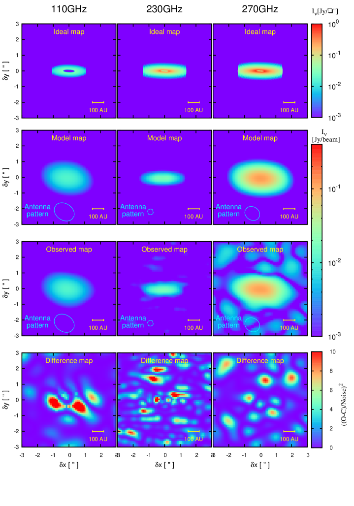
2mm normal

Figure 2: Maps of the disk radiation intensity at 110 GHz (left column), 230 GHz (central column), and 270 GHz (right column). The upper row shows the ideal disk images for observations using a telescope with a point-like beam, the second row is the ideal disk images convolved with the beam, the third row is the observed images, and the fourth row is the maps of the difference between the observed (O) and model (C) images in noise units $\sigma_{\nu}$: $\rm((O-C)/\sigma_{\nu})^{2}$.

Numerical values of some model parameters corresponding to the presented synthetic maps are given in Table 2, together with the confidence intervals calculated according to (28) and the minimum values $\chi^{2}_{\rm red}$. Note the high level of agreement between the observed and synthetic maps: the mean deviation over a map is less than 1.5 times the noise.

0mm
Parameter 110 GHz 230 GHz 270 GHz 230+270 GHz 110+230+270 GHz $\chi^{2}_{\rm red}$ 0.9 1.3 1.1 1.7 2.2 $R_{\rm in}$, AU $54^{+7}_{-3}$ $38^{+18}_{-12}$ $36^{+15}_{-13}$ 37${}^{+16}_{-14}$ 33${}^{+13}_{-15}$ $R_{\rm out}$, AU $157^{+6}_{-12}$ $204^{+161}_{-64}$ $210^{+61}_{-41}$ 222${}^{+75}_{-57}$ 207${}^{+25}_{-32}$ $\Sigma_{0}^{\rm gas}$, g/cm² $782^{+37}_{-78}$ $809^{+206}_{-218}$ $757^{+142}_{-126}$ 710${}^{+152}_{-147}$ 865${}^{+116}_{-114}$ $p$ $-0.64^{+0.02}_{-0.02}$ $-0.96^{+0.06}_{-0.06}$ $-0.87^{+0.04}_{-0.04}$ $-0.81^{+0.04}_{-0.05}$ $-0.69^{+0.03}_{-0.03}$ $i$, deg $72^{+12}_{-13}$ $78^{+12}_{-13}$ $78^{+9}_{-21}$ 78${}^{+8}_{-16}$ 82${}^{+3}_{-17}$ $f\cdot L_{\star}$ $0.03^{+0.004}_{-0.008}$ $0.15^{+0.14}_{-0.09}$ $0.12^{+0.06}_{-0.04}$ 0.08${}^{+0.05}_{-0.03}$ 0.015${}^{+0.005}_{-0.004}$ $f_{\rm Si}$ $0.38^{+0.04}_{-0.10}$ $0.49^{+0.28}_{-0.26}$ $0.47^{+0.18}_{-0.20}$ 0.59${}^{+0.19}_{-0.20}$ 0.37${}^{+0.13}_{-0.13}$ $a_{\rm max}$, cm $<1.7\cdot 10^{-2}$ $<1.4\cdot 10^{-2}$ $<1.0\cdot 10^{-2}$ $<1.3\cdot 10^{-2}$ $<1.7\cdot 10^{-2}$

Table 2: Parameters of the best-fit model.

We have analyzed in detail $\chi^{2}_{\rm red}$ as a function of a number of important parameters: $R_{\rm in}$, $i$ and $a_{\rm max}$. Figure 3 shows the dependence $\chi^{2}_{\rm red}(R_{\rm in})$ in the vicinity of the minimum, keeping the remaining parameters fixed. In this case also, the parameters obtained for 110 GHz differ appreciably from those obtained for the other two frequencies. The inner disk radius is approximately $37\pm 15$ AU at 230 and 270 GHz, and approximately $55\pm 5$ AU at 110 GHz. The presence of a dust-free region with a size of $45\pm 5$ AU was suggested in Sauter et al. (2009) based on the presence of a central plateau in the 230 GHz map. Figure 3 demonstrates that neither the new observations obtained using the PdBI (110 and 230 GHz) nor those used in Sauter et al. (2009) (obtained using the SMA at 270 GHz) can be explained without assuming the existence of a large, free-dust central region. This region could have arisen due to both dynamical effects, such as the sweeping up of dust by a binary star, and evolutionary effects, such as the formation of planetesimals in the central regions. In this case, the absence of radiation from the central region can be explained by inefficient reprocessing of the radiation from the central star, rather than an absence of matter. Such holes are often observed in other disks Dutrey et al. (2008); Brown et al. (2009).

5mm

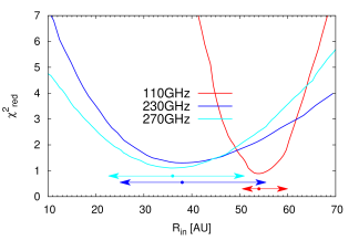
Figure 3: Fit criterion $\chi^{2}_{\rm red}$ as a function of the inner disk radius $R_{\rm in}$. The other parameters were fixed at the values reached at the minimum $\chi^{2}_{0}=\min\chi^{2}_{\rm red}$. The arrows indicate the confidence intervals corresponding to $\chi^{2}_{\rm red}=\chi^{2}_{0}+1$, and the points on the arrows correspond to the minimum.

The disk inclination $i$ is an important parameter for modeling the bipolar outflow from CB 26. The accuracy in this parameter can be estimated using Figure 4, which presents the dependence $\chi^{2}_{\rm red}(i)$ for the three frequencies. We show confidence intervals for $i<90^{\circ}$, since the southern edge of the disk is nearer to the Earth, as is suggested by observations of the outflow in molecular lines. The mean inclination over the three maps is $76^{\circ}$. None of these millimeter maps are sensitive to the edge of the disk that is nearest the observer (the symmetry of $\chi^{2}_{\rm red}(i)$ relative to $90^{\circ}$).

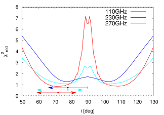
5mm normal

Figure 4: Fit criterion $\chi^{2}_{\rm red}$ as a function of the inclination angle $i$ of the disk to the plane of the sky. The other parameters were fixed at the values reached at the minimum $\chi^{2}_{0}=\min\chi^{2}_{\rm red}$. The arrows indicate the confidence intervals corresponding to $\chi^{2}_{\rm red}=\chi^{2}_{0}+1$ and $i<90^{\circ}$ (this orientation follows from observations in molecular lines). The points on the arrows correspond to the minimum. For $i<90^{\circ}$, the south pole of the disk axis is oriented toward the Earth.

Figure 6 shows the dependence $\chi^{2}_{\rm red}(a_{\rm max})$. The synthetic maps are not sensitive to the maximum size of the dust particles in the range from interstellar values to $10^{-2}$ cm. Our model suggests an upper limit to the maximum size of the dust particles in CB 26 of $0.02$ cm.

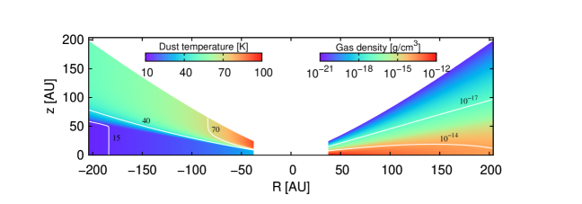
normal

Figure 5: Dust temperature (left) and gas density (right) distributions for the disk models whose best-fit parameters correspond to the observed maps at 230 and 270 GHz.

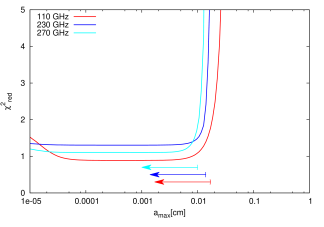
5mm normal

Figure 6: Fit criterion $\chi^{2}_{\rm red}$ as a function of the maximum size of the dust particles $a_{\rm max}$. The other parameters were fixed at the values reached at the minimum $\chi^{2}_{0}=\min\chi^{2}_{\rm red}$. The arrows indicate the confidence intervals corresponding to $\chi^{2}_{\rm red}=\chi^{2}_{0}+1$.

6.2 Combined Model

The fifth column in Table 2 presents the model parameters determined using the 230 and 270 GHz maps jointly. The maps at these two frequencies obtained with different angular resolutions using different instruments yield quite similar disk parameters, whereas the 110 GHz map gives different parameters and shows the presence of correlated features in the residuals (Figure 2). Therefore, we excluded the 110 GHz map from our final search for the disk parameters. The mean value of $\chi^{2}_{\rm red}=(\chi^{2}_{\rm 230}+\chi^{2}_{\rm 270})/2$ was used for $\chi^{2}_{\rm red}$. The results obtained using all three maps are given in the last column of Table 2 for comparison.

The physical structure of the disk corresponding to the joint minimum $\chi^{2}_{\rm red}$ is shown in Figure 5. The dust temperature varies from 10 K in the peripheral regions near the equatorial plane to 100 K in the atmosphere of the disk at its center. The maximum gas density in the equatorial plane reaches $10^{-12}$ g/cm³. The normalized surface density, power-law index, and portion of the stellar radiation intercepted by the disk are $\Sigma_{0}^{\rm gas}=710$ g/cm², $p=-0.8$, and $fL_{\star}=0.08L_{\odot}$. The full optical depth of the disk is close to unity at all three frequencies. The maximum optical depth is reached in the vicinity of the disk inner boundary, and is equal to 0.35, 0.6, and 0.9 for 110, 230, and 270 GHz, correspondingly.

6.3 Model Degeneracy

The fact that we observe the disk edge-on and cannot see the direct radiation from the star hinders determination of the spectral type of the central star. The lack of information about the effective temperature of the star means that the thermal structure of the disk must be reconstructed, and the characteristic dust temperature required to determine the disk mass Andrews and Williams (2005) must be estimated. There is a fundamental (physical) constraint on the joint, simultaneous determination of the mass and characteristic temperature of the disk in the case of spatially unresolved observations in the millimeter. We constructed maps of $\chi^{2}_{\rm red}$ as functions of the structural parameters in order to study the degeneracy of spatially resolved observations. Figure 7 shows $\chi^{2}_{\rm red}$ as functions of the normalization of the surface density $\Sigma_{0}^{\rm gas}$ and the portion of the stellar radiation intercepted by the disk $fL_{\star}$. For ease of viewing, the latter quantity has been transformed to the effective temperature of the star using the standard formula $fL_{\star}=f4\pi R_{\rm star}^{2}\cdot\sigma_{B}T_{\rm star}^{4}$ for $R_{\rm star}=R_{\odot},f=0.1$. The values of parameters from the dark-grey region with $\chi^{2}_{\rm red}\lesssim 2$ (Figure 7) describe the observations equally well. This region of parameters can be described by the law $\Sigma_{0}^{\rm gas}T^{\alpha}={\rm const}$, where $\alpha=1.3\div 1.7$. $\chi^{2}_{\rm red}$ behaves similarly in the $\left(\Sigma_{0}^{\rm gas},p\right)$ parameter plane (Figure 8), with the steeper decrease in the surface density toward the periphery corresponding to greater values of $\Sigma_{0}^{\rm gas}$.

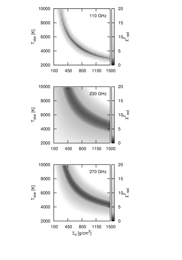
5mm normal

Figure 7: Fit criterion $\chi^{2}_{\rm red}$ as a function of the normalization of the surface density $\Sigma_{0}^{\rm gas}$ and the temperature $T_{\rm star}$ of the central star.

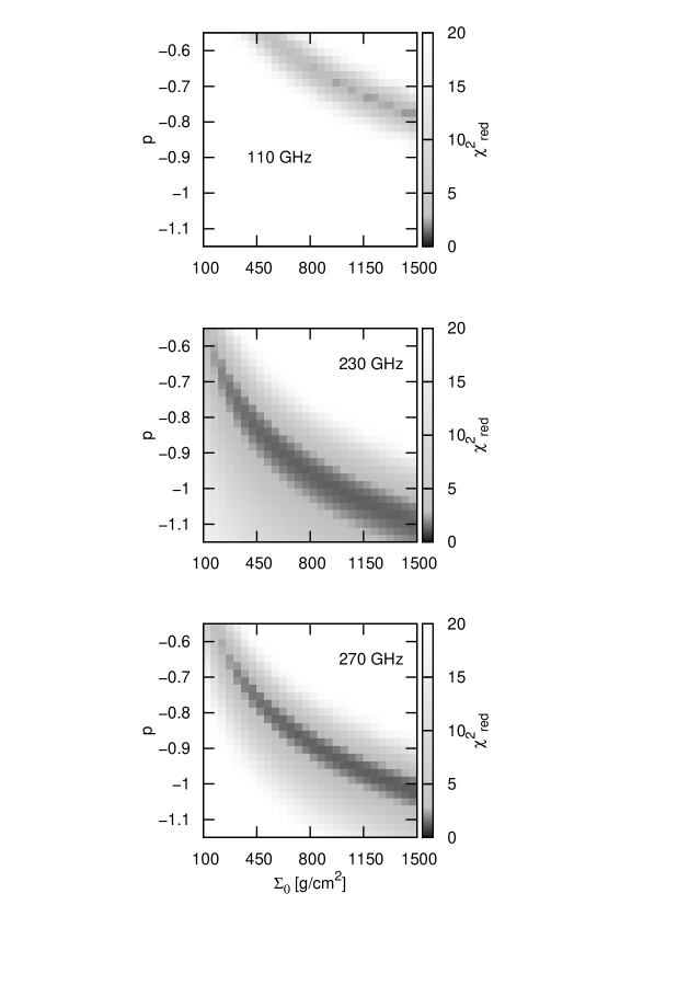
5mm normal

Figure 8: Fit criterion $\chi^{2}_{\rm red}$ as a function of the normalization of the surface density $\Sigma_{0}^{\rm gas}$ and the index $p$ of the power-law function for $\Sigma_{\rm T}$.

6.4 Origin of the Differences of 110 GHz Map

5mm normal

Figure 9: SED of CB 26. The open circles show the data from which the envelope’s contribution has been subtracted. For ease of viewing, the straight line shows the slope of the Rayleigh–Jeans part of the spectrum, derived using the last four points, except for 110 GHz.

All the available data indicate that the 110 GHz map (corresponding to longest of the wavelengths considered) differs from the remaining two. First, the residuals display correlated features within the disk image (Figure 2), suggesting a systematic difference between the observational and theoretical data at this frequency, or that the derived $\chi^{2}_{\rm red}$ represents a local minimum. Second, the disk parameters derived using this map differ appreciably from those obtained using the 230 and 270 GHz maps (Table 2). Third, if the point corresponding to 110 GHz is plotted on the SED (Figure 9), it deviates appreciably from the straight line in the Rayleigh–Jeans part of the spectrum. To plot Figure 9 we used the fluxes from Sauter et al. (2009) together with data from the Herschel. The deviation of a linear SED and the differences in the disk parameters at 110 GHz and at the other frequencies can be explained in the following way:

• there exists an additional radiative mechanism that is not taken into account in the model, which is not important at high frequencies, but becomes appreciable at 110 GHz (e.g., free–free radiation arising in the accretion region or bipolar outflow);

• an envelope around the disk could also contribute to the radiation, since the 110 GHz beam is larger than the 230 and 270 GHz beams (we are planning to use CO line observations to estimate the envelope’s contribution);

• it is difficult to establish an accurate dust model (chemical composition and extinction efficiency coefficients).

These (or other) effects could result in the overall difference between the 110 GHz map and the maps at 230 and 270 GHz. It seems reasonable to use the results based on the latter two maps (rather than all three) as a final disk model, until we determine the nature of the operating additional mechanism and take it into account.

7 CONCLUSIONS

The appearance of modern radio interferometers with high sensitivities and good angular resolutions (SMA, Plateau de Bure, CARMA, ALMA) has made it possible to obtain spatially resolved images of protoplanetary disks. The reconstruction of the physical structures of the disks from these observations is a challenging task that requires an integrated approach, that is simultaneously self-consistent physically and correct mathematically, aimed at modeling and fitting the observations. One of the main goals of this paper was to develop such an approach.

The key characteristic of the protoplanetary disk model we used to reconstruct the disk parameters is a compromise between the completeness of the description provided and the time required to compute the physical structure of the disk. The use of a two-frequency approximation and the corresponding mean opacities in the radiative transfer model, as well as the iterative scheme employed to solve the equation of hydrostatic equilibrium, yield a short model computation time. Together with the rapid computation of the theoretical maps, the adaptive algorithm for convolution of the images with the beam, and the efficient method used to minimize $\chi^{2}_{\rm red}$, this made it possible to use the developed code to search for best-fit model parameters of the disk.

We applied this code to determine the physical structure of the protoplanetary disk in CB 26 using interferometric images in the millimeter. Observational data at 110, 230, and 270 GHz from the SMA, IRAM Plateau de Bure, and OVRO interferometers were used to search for best-fit models. Best-fit model parameters were obtained for each of the frequencies, for all the frequencies jointly, and for 230 and 270 GHz jointly. All three observational maps suggest the existence of a central, dust-free region in the disk, approximately 35 AU in radius. This corresponds well to the value of 45 AU obtained in Sauter et al. (2009) at 230 GHz. However, our simulated maps yield a disk inclination of $78^{\circ}$, which is lower than the value of $85^{\circ}$ used in Launhardt et al. (2009). This should lead to an appreciable decrease in the bipolar outflow velocity for the model Launhardt et al. (2009), and to a lower rate of angular momentum transfer from the disk. We cannot determine whether or not the dust particles in the disk can grow appreciably in size (see also Sauter et al. (2009)); we can only establish an upper bound on the dust size ($a_{\rm max}<0.02$ cm) using our dust model, comprising a mixture of silicate and graphite particles with a power-law size distribution.

We came across the following difficulties when simulating CB 26. The 110 GHz map stands out from the others due to the change in the SED slope, the presence of symmetrical features in the residual map within the disk image, and differences in the physical parameters implied by the best-fit model. These may indicate that (a) the model does not include free–free radiation, although this may be comparable with the thermal radiation of the disk at longer wavelengths; (b) the contribution from a disk envelope has been neglected; (c) the dust model is not sufficiently realistic. All these factors must be considered in more detail. Our analysis also indicates a wide region of degeneracy between the thermal and density characteristics of the disk. In our opinion, this is a fundamental problem hindering our ability to unambiguously establish the disk parameters. This problem can be avoided in objects, in which the radiation of the central star is not screened by the circumstellar disk, and the stellar parameters can be determined independently. It is also obvious that an increase in angular resolution is necessary for this degeneracy to be removed. We plan to study in future whether or not the region of parameter degeneracy can be diminished using maps from other wavebands.

Translated by N. Lipunova