Type-I Intermittency With Noise
Versus Eyelet Intermittency

Abstract

In this article we compare the characteristics of two types of the intermittent behavior (type-I intermittency in the presence of noise and eyelet intermittency taking place in the vicinity of the chaotic phase synchronization boundary) supposed hitherto to be different phenomena. We show that these effects are the same type of dynamics observed under different conditions. The correctness of our conclusion is confirmed by the consideration of different sample systems, such as quadratic map, Van der Pol oscillator and Rössler system. Consideration of the problem concerning the upper boundary of the intermittent behavior also confirms the validity of the statement on the equivalence of type-I intermittency in the presence of noise and eyelet intermittency observed in the onset of phase synchronization.

Introduction

Intermittency is well-known to be an ubiquitous phenomenon in nonlinear science. Its arousal and main statistical properties have been studied and characterized already since long time ago, and different types of intermittency have been classified as types I–III intermittencies [1, 2], on–off intermittency [3, 4], eyelet intermittency [5, 6, 7] and ring intermittency [8].

Despite of some similarity (the presence of two different regimes alternating suddenly with each other in the time series), every type of intermittency is governed by its own certain mechanisms and characteristics of the intermittent behavior (such as the dependence of the mean length of the laminar phases on the control parameter, the distribution of the laminar phase lengths, etc.) of different intermittency types are distinct. There are no doubts that different types of intermittent behavior may take place in a wide spectrum of systems, including cases of practical interest for applications in radio engineering, medical, physiological, and other applied sciences.

This article is devoted to the comparison of characteristics of type-I intermittency in the presence of noise and eyelet intermittency taking place in the vicinity of the phase synchronization boundary. Although these types of intermittency are known to be characterized by different theoretical laws, we show here for the first time that these two types of the intermittent behavior considered hitherto as different phenomena are, in fact, the same type of the system dynamics.

The structure of the paper is the following. In Sec. 1 we give the brief theoretical data concerning both the type-I intermittency with noise and eyelet intermittency observed in the vicinity of the phase synchronization boundary as well as arguments confirming the equivalence of these types of the dynamics. The next Sections 2–3 aim to verify the statement given in the Sec. 1 by means of numerical simulations of the dynamics of several model systems such as a quadratic map, Rössler oscillators, etc. Eventually, in Sec. 4 we discuss the problem of the upper boundary of the intermittent behavior. The final conclusions are given in Sec. 5.

1 Relation between type-I intermittency with noise and eyelet intermittency

First, we consider briefly both eyelet intermittency in the vicinity of the phase synchronization boundary and type-I intermittency in the presence of noise following conceptions accepted generally. The main arguments confirming equivalence of these types of the intermittent behavior are given afterwards.

1.1 Type-I intermittency with noise

The intermittent behavior of type-I is known to be observed below the saddle-node bifurcation point, with the mean length of laminar phases $T$ being inversely proportional to the square root of the criticality parameter $(\varepsilon_{c}-\varepsilon)$, i.e.

$$T\sim(\varepsilon_{c}-\varepsilon)^{-1/2},$$ (1)

where $\varepsilon$ is the control parameter and $\varepsilon_{c}$ is its bifurcation value corresponding to the bifurcation point [9]. The influence of noise on the system results in the transformation of characteristics of intermittency [10, 11, 12], with the intermittent behavior being observed in this case both below and above the saddle-node bifurcation point $\varepsilon_{c}$. In the supercritical region [12] of the control parameter values (i.e., above the point of bifurcation, ${\varepsilon>\varepsilon_{c}}$) the mean length $T$ of the laminar phases is given by

$$T=\frac{1}{k\sqrt{\varepsilon-\varepsilon_{c}}}\exp\left(\frac{4(\varepsilon-\varepsilon_{c})^{3/2}}{3D}\right),$$ (2)

where $k=\mathrm{const}$, $D$ is the intensity of a delta-correlated white noise $\xi_{n}$ [${\langle\xi_{n}\rangle=0}$, ${\langle\xi_{n}\xi_{m}\rangle=D\delta(n-m)}$], with Equation (2) being applicable in the region

$$D^{2/3}\ll|\varepsilon-\varepsilon_{c}|\ll 1$$ (3)

of the control parameter plane [10, 13]. In this region the criticality parameter ${(\varepsilon-\varepsilon_{c})}$ is large enough and, therefore, the approximate equation

$$\ln T=B(\varepsilon-\varepsilon_{c})^{3/2}-\ln k$$ (4)

(where $B=\mathrm{const}$) is used typically (see [11] for detail) instead of (2). In turn, the distribution $p(\tau)$ of the laminar phase lengths $\tau$ is governed by the exponential law [12]

$$p(\tau)=T^{-1}\exp\left(-{\tau/T}\right).$$ (5)

1.2 Eyelet intermittency

For the chaotic systems in the vicinity of the phase synchronization boundary (if the natural frequencies of oscillator and external signal are detuned slightly) two types of the intermittent behavior and, correspondingly, two critical values are reported to exist [5, 14, 6]. Below the boundary of the phase synchronization regime the dynamics of the phase difference $\Delta\varphi(t)$ features time intervals of the phase synchronized motion (laminar phases) persistently and intermittently interrupted by sudden phase slips (turbulent phases) during which the value of $|\Delta\varphi(t)|$ jumps up by $2\pi$. For two coupled chaotic systems there are two values of the coupling strength $\varepsilon_{1}<\varepsilon_{2}$ being the characteristic points which are considered to separate the different types of the dynamics. Below the coupling strength value $\varepsilon_{1}$ the type-I intermittency is observed, with the power law $T\sim(\varepsilon_{1}-\varepsilon)^{-1/2}$ taking place for the mean length of the laminar phases, whereas above the critical point $\varepsilon_{2}$ the phase synchronization regime is revealed. For the coupling strength $\varepsilon\in(\varepsilon_{1};\varepsilon_{2})$ the super-long laminar behavior (the so called “eyelet intermittency”) should be detected. For eyelet intermittency (see, e.g. [5, 6]) the dependence of the mean length $T$ of the laminar phases on the criticality parameter is expected to follow the law

$$T\sim\exp\left(\kappa(\varepsilon_{2}-\varepsilon)^{-1/2}\right)$$ (6)

or

$$\ln(1/T)=c_{0}-c_{1}(\varepsilon_{2}-\varepsilon)^{-1/2},$$ (7)

($c_{0}$, $c_{1}$ and $\kappa$ are the constants) given for the first time in [15] for the transient statistics near the unstable-unstable pair bifurcation point. The analytical form of the distribution of the laminar phase lengths has not been reported anywhere hitherto for eyelet intermittency.

The theoretical explanation of the eyelet intermittency phenomenon is based on the boundary crisis of the synchronous attractor caused by the unstable-unstable bifurcation when the saddle periodic orbit and repeller periodic orbit join and disappear [5, 14]. This type of the intermittent behavior has been observed both in the numerical calculations [5, 6] and experimental studies [7] for the different nonlinear systems, including Rössler oscillators.

1.3 Theory of equivalence of the considered types of behavior

Although type-I intermittency with noise and eyelet intermittency taking place in the vicinity of the chaotic phase synchronization onset seem to be different phenomena, they are really the same type of the dynamics observed under different conditions. The difference between these types of the intermittent behavior is only in the character of the external signal. In case of the type-I intermittency with noise the stochastic signal influences on the system, while in the case of eyelet intermittency the signal of chaotic dynamical system is used to drive the response chaotic oscillator. At the same time, the core mechanism governed the system behavior (the motion in the vicinity of the bifurcation point disturbed by the stochastic or deterministic perturbations) is the same in both cases. To emphasize the weak difference in the character of the driving signal we shall further use the terms “type-I intermittency with noise” and “eyelet intermittency” despite of the fact of the equivalence of these types of the intermittent behavior.

Indeed, the phenomena observed near the synchronization boundary for periodic systems whose motion is perturbed by noise (in other words, the behavior in the vicinity of the saddle-node bifurcation perturbed by noise) have been shown recently to be the same as for chaotic oscillators in the vicinity of the phase synchronization boundary [16, 13, 5, 12]. Thus, both for two coupled chaotic Rössler systems and driven Van der Pol oscillator the same scenarios of the synchronous regime destruction have been revealed [16]. Moreover, for two coupled Rössler systems the behavior of the conditional Lyapunov exponent in the vicinity of the onset of the phase synchronization regime is governed by the same laws as in the case of the driven Van der Pol oscillator in the presence of noise [13]. Additionally, when the turbulent phase begins the phase trajectory demonstrates motion being close to periodic both for the eyelet intermittency observed in the vicinity of the phase synchronization boundary (see [14]) and for type-I intermittency with noise. Finally, the repeller and saddle periodic orbits of the same period in the vicinity of the parameter region corresponding to the intermittent behavior tend to coalesce with each other (see, e.g. [5, 12]) for both these types of the intermittent behavior. Obviously, if the phenomena observed near the saddle-node bifurcation point for the systems whose motion is perturbed by noise are the same as for chaotic oscillators in the vicinity of the phase synchronization onset, one can expect that the intermittent behavior of two coupled chaotic oscillators near the phase synchronization boundary (eyelet intermittency) is also exactly the same as intermittency of type-I in the presence of noise in the supercritical region.

So, if type-I intermittency with noise and eyelet intermittency taking place in the vicinity of the chaotic phase synchronization onset are the same type of the system dynamics, the theoretical equations (4) and (7) obtained for these types of the intermittent behavior are the approximate expressions being the different forms of Eq. (2) describing the dependence of the mean length of the laminar phases on the criticality parameter. Therefore, Eq. (7) can be deduced from Eq. (4) and vice versa. As a consequence, the coefficients $B$, $k$ and $c_{0}$, $c_{1}$ in (4) and (7) are related with each other. Obviously, the mean length of the laminar phases must obey Eq. (4) and Eq. (7) simultaneously, independently whether the system behavior is classified as eyelet intermittency or type-I intermittency with noise. Additionally, the laminar phase length distribution for the considered type of behavior must satisfy the exponential law (5).

The intermittent behavior under study is considered in the coupling strength range ${\varepsilon_{c}<\varepsilon<\varepsilon_{2}}$. In the case of the system driven by external noise (type-I intermittency with noise) the lower boundary value $\varepsilon_{c}$ corresponds to the saddle-node bifurcation point when external noise is switched off. For the dynamical systems demonstrating the chaotic behavior (eyelet intermittency) the lower boundary $\varepsilon_{c}$ may be found, e.g., in the way described in [13]. As far as the choice of the upper boundary value $\varepsilon_{2}$ is concerned, this subject is discussed in detail in Sec. 4 of this paper both for chaotic and stochastic external signals.

To find the relationship between coefficients in (4) and (7) we introduce the auxiliary variable $\xi=(\varepsilon_{2}-\varepsilon)^{-1/2}$ and expand $\ln(1/T)$ determined by Eq. (4) (type-I intermittency with noise) into Taylor series in the vicinity of the point $\xi_{0}=(\varepsilon_{2}-\varepsilon_{0})^{-1/2}$, where ${\varepsilon_{c}<\varepsilon_{0}<\varepsilon_{2}}$, i.e.

$$\begin{array}[]{ll}\displaystyle\ln\left(1/T\right)&=\left(\ln k-B(\varepsilon_{0}-\varepsilon_{c})^{3/2}\right)-\\ \\ &-3\left(B\sqrt{\varepsilon_{0}-\varepsilon_{c}}\left(\varepsilon_{2}-\varepsilon_{0}\right)^{3/2}\right)(\xi-\xi_{0})+\\ \\ &\displaystyle+\frac{3B(\varepsilon_{2}-\varepsilon_{0})^{2}(4\varepsilon_{0}-\varepsilon_{2}-3\varepsilon_{c})}{2\sqrt{\varepsilon_{0}-\varepsilon_{c}}}(\xi-\xi_{0})^{2}+o\left((\xi-\xi_{0})^{3}\right)=\\ \\ &\displaystyle=\ln k-\frac{B\left(20\varepsilon_{0}^{2}-21\varepsilon_{0}\varepsilon_{2}+3\varepsilon_{2}^{2}-19\varepsilon_{c}\varepsilon_{0}+15\varepsilon_{c}\varepsilon_{2}+2\varepsilon_{c}^{2}\right)}{2\sqrt{\varepsilon_{0}-\varepsilon_{c}}}\\ \\ &\displaystyle-\frac{3B\left(\varepsilon_{2}-\varepsilon_{0}\right)^{2}(5\varepsilon_{0}-\varepsilon_{2}-4\varepsilon_{c})}{\sqrt{\varepsilon_{0}-\varepsilon_{c}}\sqrt{\varepsilon_{2}-\varepsilon_{0}}}(\varepsilon_{2}-\varepsilon)^{-1/2}+\\ \\ &\displaystyle+\frac{3B\left(\varepsilon_{2}-\varepsilon_{0}\right)^{2}(4\varepsilon_{0}-\varepsilon_{2}-3\varepsilon_{c})}{2\sqrt{\varepsilon_{0}-\varepsilon_{c}}}(\varepsilon_{2}-\varepsilon)^{-1}+o\left((\xi-\xi_{0})^{3}\right).\end{array}$$ (8)

Having neglected the term $o\left((\xi-\xi_{0})^{3}\right)$ in (8) one can write Eq. (8) in the form

$$\ln(1/T)=c_{0}-c_{1}(\varepsilon_{2}-\varepsilon)^{-1/2}+c_{2}(\varepsilon_{2}-\varepsilon)^{-1}.$$ (9)

Having required

$$c_{2}=\frac{3B\left(\varepsilon_{2}-\varepsilon_{0}\right)^{2}(4\varepsilon_{0}-\varepsilon_{2}-3\varepsilon_{c})}{2\sqrt{\varepsilon_{0}-\varepsilon_{c}}}\equiv 0$$ (10)

we obtain, that

$$\varepsilon_{0}=\frac{\varepsilon_{2}+3\varepsilon_{c}}{4},\qquad\varepsilon_{c}<\varepsilon_{0}<\varepsilon_{2}$$ (11)

and, therefore, equation (9) describing the dependence of the mean length $T$ of the laminar phases on the criticality parameter for type-I intermittency with noise coincides exactly with Eq. (7) corresponding to eyelet intermittency. Correspondingly, in terms of Eq. (11) the relationship between coefficients $B$, $k$ and $c_{0}$, $c_{1}$ in (4) and (7) is the following

$$\begin{array}[]{ll}c_{0}&=\ln k+B(\varepsilon_{2}-\varepsilon_{c})^{3/2},\\ \\ \displaystyle c_{1}&=\frac{\displaystyle 9\sqrt{3}}{\displaystyle 16}B(\varepsilon_{2}-\varepsilon_{c})^{2}.\end{array}$$ (12)

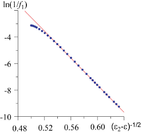
Figure 1: The dependence ${f_{1}(\varepsilon)=k^{-1}\exp(B\varepsilon^{3/2})}$ simulating the theoretical law (4) and its approximation by the curve $f_{2}(x)=c_{0}-c_{1}(\varepsilon-\varepsilon_{2})^{-1/2}$ corresponding to law (7) for eyelet intermittency. The parameter values are $k^{-1}=23$, $B=3.33$, $c_{0}=23.5$, $c_{1}=51.9$, $x_{2}=4.0$. The points corresponding to $f_{1}(x)$ are shown by symbols $\bullet$. The theoretical law (7) for eyelet intermittency is shown by the solid line

Fig. 1 illustrates the relationship of two theoretical laws (4) and (7) in the region $\varepsilon>\varepsilon_{c}$. Here function $f_{1}(x)=k^{-1}\exp(B\varepsilon^{3/2})$ simulates the theoretical law (4) (the critical point is supposed to be $\varepsilon_{c}=0$), whereas the curve $f_{2}(x)=c_{0}-c_{1}(\varepsilon-\varepsilon_{2})^{-1/2}$ corresponds to law (7) for eyelet intermittency. The value of coefficients $B$, $k$, $c_{0}$ and $c_{1}$ have been selected according to Eq. (12). One can see that in the region of the study both curves coincide with each other. It means that the mean length of the laminar phases obeys Eq. (4) and Eq. (7) simultaneously, independently whether the system behavior is classified as eyelet intermittency or type-I intermittency with noise.

2 Numerical verifications

To confirm the concept of the equivalence of intermittencies being the subject of this study we consider several examples of the intermittent behavior classified both as eyelet intermittency taking place in the vicinity of the phase synchronization onset (two coupled Rössler systems) and type-I intermittency with noise (quadratic map and driven Van der Pol oscillator).

2.1 Two coupled Rössler systems

As we have mentioned above, the intermittent behavior of two coupled chaotic oscillators in the vicinity of the phase synchronization boundary is classified traditionally as eyelet intermittency [5, 14, 6]. Nevertheless, the behavior of two coupled Rössler oscillators close to the phase synchronization onset was considered from the point of view of type-I intermittency with noise for the first time in [11], whereas the same dynamics from the position of eyelet intermittency was studied in [6]. According to different works the mean length of laminar phases happens to satisfy both Eq. (4) (Ref. [11]) and Eq. (7) (Ref. [6]). Recently [17] the distribution of the laminar phase lengths has been found to obey the exponential law (5) corresponding to type-I intermittency with noise. To give the complete picture we replicate the consideration of two coupled Rössler systems near the onset of the phase synchronization regime for the different type of coupling between oscillators and another set of the control parameter values and show that the observed intermittent behavior may be classified both as eyelet intermittency and type-I intermittency with noise.

The system under study is represented by a pair of unidirectionally coupled Rössler systems, whose equations read as

$$\begin{array}[]{l}\dot{x}_{d}=-\omega_{d}y_{d}-z_{d},\\ \dot{y}_{d}=\omega_{d}x_{d}+ay_{d},\\ \dot{z}_{d}=p+z_{d}(x_{d}-c),\\ \\ \dot{x}_{r}=-\omega_{r}y_{r}-z_{r}+\sigma(x_{d}-x_{r}),\\ \dot{y}_{r}=\omega_{r}x_{r}+ay_{r},\\ \dot{z}_{r}=p+z_{r}(x_{r}-c),\\ \end{array}$$ (13)

where $(x_{d},y_{d},z_{d})$ [$(x_{r},y_{r},z_{r})$] are the Cartesian coordinates of the drive [the response] oscillator, dots stand for temporal derivatives, and $\sigma$ is a parameter ruling the coupling strength. The other control parameters of Eq. (13) have been set to $a=0.15$, $p=0.2$, $c=10.0$, in analogy with our previous studies [18, 19]. The $\omega_{r}$–parameter (representing the natural frequency of the response system) has been selected to be $\omega_{r}=0.95$; the analogous parameter for the drive system has been fixed to $\omega_{d}=0.93$. For such a choice of the control parameter values, both chaotic attractors of the drive and response systems are phase coherent. The instantaneous phase of the chaotic signals $\varphi(t)$ can be therefore introduced in the traditional way as the rotation angle ${\varphi_{d,r}=\arctan(y_{d,r}/x_{d,r})}$ on the projection plane $(x,y)$ of each system.

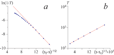
Figure 2: The points obtained numerically for two unidirectionally coupled Rössler oscillators (13) are shown by symbols “$\bullet$”. The theoretical laws (7) and (4) are shown by the solid lines. (a) Eyelet intermittency: the dependence of $\ln(1/T)$ on the parameter ${(\sigma_{2}-\sigma)^{-1/2}}$; $\sigma_{2}=0.042$, $c_{0}=-0.75$, $c_{1}=0.55$. (b) Type-I intermittency with noise: the dependence of the mean laminar phase length $T$ on the parameter ${(\sigma-\sigma_{c})^{3/2}}$, with the ordinate axis being shown in the logarithmic scale; $\sigma_{c}=0.0345$, $B=1.01\times 10^{4}$, $k=6.68\times 10^{-4}$

In Fig. 2 one and the same result of the numerical simulation of two coupled Rössler systems (13) is shown in different ways to compare obtained data with the analytical predictions (7) and (4) for eyelet intermittency taking place near the phase synchronization boundary (Fig. 2, a) and type-I intermittency with noise (Fig. 2, b), respectively. The dependence of $T$ on ${(\sigma_{2}-\sigma)}$ is shown in the whole range of the coupling parameter strength values (Fig. 2, a) to make evident the deviation of numerically obtained data from law (7) far away from the onset of the phase synchronization. The coupling strength $\sigma$ plays the role of the control parameter. The critical point $\sigma_{2}\approx 0.042$ relates to the onset of the phase synchronization regime in two coupled Rössler systems. The point $\sigma_{c}\approx 0.0345$ used in (2) and (4) corresponds to the saddle-node bifurcation point if the chaotic dynamics being the analog of noise could be switched off. The value of this point has been found from the dependence of the zero conditional Lyapunov exponent on the coupling strength (see for detail [13]).

One can see, that the intermittent behavior of two coupled Rössler systems may be treated both as eyelet and noised type-I intermittency with the excellent agreement between numerical data and theoretical curve in both cases. Moreover, the coefficients $c_{0}$, $c_{1}$ and $B$, $k$ of the theoretical equations (7) and (4) agree very well with each other according to Eq. (12). It allows us to state that both these effects are the same type of the system dynamics. Nevertheless, to be totaly convinced of the correctness of our decision we have to consider other examples of the intermittent behavior classified traditionally (contrary to the previous case of two coupled Rössler systems) as type-I intermittency with noise.

2.2 Driven Van der Pol oscillator with noise

The second sample dynamical system to be considered is Van der Pol oscillator

$${\ddot{x}-(\lambda-x^{2})\dot{x}+x=A\sin(\omega_{e}t)+D\xi(t)}$$ (14)

driven by the external harmonic signal with the amplitude $A$ and frequency $\omega_{e}$ with the added stochastic term $D\xi(t)$. The values of the control parameters have been selected as $\lambda=0.1$, $\omega_{e}=0.98$. For the selected values of the control parameters and $D=0$ the dynamics of the driven Van der Pol oscillator becomes synchronized when ${A=A_{c}=0.0238}$ that corresponds to the saddle-node bifurcation. The probability density of the random variable $\xi(t)$ is

$$p(\xi)=\frac{1}{\sqrt{2\pi}\sigma}\exp\left(-\frac{\xi^{2}}{2\sigma^{2}}\right),$$ (15)

where $\sigma^{2}=1$. To integrate Eq. (14) the one-step Euler method has been used with time step $h=5\times 10^{-4}$, the value of the noise intensity has been fixed as $D=1$.

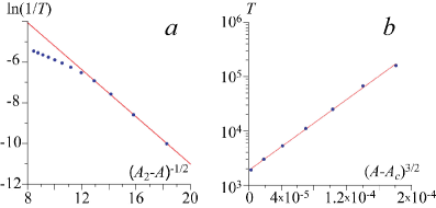
Figure 3: The points obtained numerically for driven Van der Pol oscillator with the stochastic force (14) are shown by symbols “$\bullet$”. The theoretical laws (7) and (4) are shown by the solid lines. (a) Eyelet intermittency: the dependence of $\ln(1/T)$ on the parameter ${(A_{2}-A)^{-1/2}}$; $A_{2}=0.029$, $c_{0}=1.24$, $c_{1}=0.62$. (b) Type-I intermittency with noise: the dependence of the mean laminar phase length $T$ on the parameter ${(A-A_{c})^{3/2}}$; $A_{c}=0.0238$, $B=2.37\times 10^{4}$, $k=4.76\times 10^{-4}$

On the one hand, as it has been discussed above, the intermittent behavior in this case have to be classified as type-I intermittency with noise. The corresponding dependence of the mean length of laminar phases on the criticality parameter ${(A-A_{c})}$ is shown in Fig. 3, b. If the amplitude $A$ of the external signal exceeds the critical value $A_{c}$ the exponential law ${T\sim\exp(\alpha(A-A_{c})^{3/2})}$ is expected to be observed. To make this law evident the abscissa in Fig. 3, b has been selected in the $(A-A_{c})^{3/2}$-scale and the ordinate axis $T$ is shown in the logarithmic scale. One can see again the excellent agreement between the numerically calculated data and theoretical prediction (4). The distribution of the lengths of the laminar phases $p(t)$ obtained for $A>A_{c}$ also confirms the theoretical curve (5), see Fig. 7 in [12].

On the other hand, trying to choose the corresponding values of $A_{2}$ for the driven Van der Pol oscillator (14) one can find out that the intermittent behavior of this system also may be identified as eyelet intermittency. Indeed, in Fig. 3, a one can see a very good agreement between the numerically obtained mean length $T$ of the laminar phases for the different values of the coupling parameter and theoretical law (7) corresponding to the eyelet intermittency. Note also, that for the well chosen values of $A_{2}$ the dependence $T(A_{2}-A)$ in the axes $((A_{2}-A)^{-1/2},\ln(1/T))$ behaves in the same way as the corresponding function $T(\sigma_{2}-\sigma)$ in the axes $((\sigma_{2}-\sigma)^{-1/2},\ln(1/T))$ for two coupled Rössler systems (13). Again, as well as for two coupled Rössler oscillators, the coefficients $c_{0}$, $c_{1}$ and $B$, $k$ of the theoretical equations (7) and (4) agree very well with each other according to Eq. (12).

2.3 Quadratic map with stochastic force

The next example is the quadratic map

$$x_{n+1}=x_{n}^{2}+\lambda-\varepsilon+D\xi_{n},\qquad\mathrm{mod}~{}1,$$ (16)

where the operation of “$\mathrm{mod~{}}1$” is used to provide the return of the system in the vicinity of the point $x=0$, ${\lambda=0.25}$ and the probability density of the stochastic variable $\xi$ is distributed uniformly throughout the interval ${\xi\in[-1,1]}$. If the intensity of noise $D$ is equal to zero the saddle-node bifurcation is observed for $\varepsilon=0$. The intermittent behavior of type-I is observed for $\varepsilon<0$, whereas the stable fixed point takes place for $\varepsilon>0$. Having added the stochastic force (${D>0}$) in (16) we suppose that the intermittent behavior must be also observed in the area of the positive values of the criticality parameter $\varepsilon$, with the mean length of the laminar phases obeying law (4).

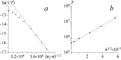
Figure 4: The points obtained numerically for quadratic map (16) are shown by symbols “$\bullet$”. The theoretical laws (7) and (4) are shown by the solid lines. (a) Eyelet intermittency: the dependence of $\ln(1/T)$ on the parameter ${(\varepsilon_{2}-\varepsilon)^{-1/2}}$; $\varepsilon_{2}=10^{-9}$, $c_{0}=7.9$, ${c_{1}=6.45\times 10^{-4}}$. (b) Type-I intermittency with noise: the dependence of the mean laminar phase length $T$ on the parameter ${\varepsilon^{3/2}}$; $\varepsilon_{c}=0$, $D=10^{-7}$, $B=6.62\times 10^{14}$, $k=2.35\times 10^{-6}$

Although in this case we deal with type-I intermittency with noise, the numerically obtained points corresponding to the mean length of laminar phases are approximated successfully both by Eq. (7) and (4) (see Fig. 4), with the coefficients $c_{0}$, $c_{1}$ and $B$, $k$ of the theoretical equations (7) and (4) agreeing with each other according to Eq. (12). These findings confirm our statement about identity of the considered types of the intermittent behavior.

So, having studied the intermittent behavior of different systems which (based on the prior knowledge) should be classified either eyelet intermittency in the vicinity of the phase synchronization boundary or type-I intermittency with the presence of noise, we can conclude that the obtained characteristics are exactly the same in all cases described above. Two next sections are devoted to the consideration of another systems to give the additional proofs of the correctness of the introduced concept.

3 Van der Pol oscillator driven by the chaotic signal

In this section we consider Van der Pol oscillator driven by the chaotic signal of Rössler system

$$\begin{array}[]{l}\dot{x}_{d}=\alpha(-\omega y-z),\\ \dot{y}_{d}=\alpha(\omega x+ay),\\ \dot{z}_{d}=\alpha(p+z(x-c)),\\ \ddot{u}-(\lambda-u^{2})\dot{u}+u=\varepsilon(Dy-\dot{u}),\\ \end{array}$$ (17)

where ${a=0.15}$, ${p=0.2}$, ${c=10}$, $\lambda=0.1$, $\omega=0.9689$ are the control parameters. The auxiliary parameters $\alpha=0.99$ and $D=0.0664$ alter the characteristics (the amplitude and main frequency) of the chaotic signal influencing on Van der Pol oscillator.

From the formal point of view the behavior of system (17) can be classified neither eyelet intermittency nor type-I intermittency with noise. Indeed, since the response oscillator is periodic there are no unstable periodic orbits embedded into its attractor to be synchronized, therefore, the system dynamics can not be considered as eyelet intermittency. Alternatively, due to the presence of chaotic perturbations there is no pure saddle-node bifurcation in this system to say about type-I intermittency. Nevertheless, it is intuitively clear that this example is nearly related to all cases considered above and one can expect to observe here the same type of intermittency as before.

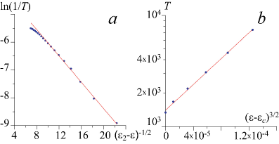
Figure 5: The points obtained numerically for Van der Pol oscillator driven by chaotic signal of Rössler system (17) are shown by symbols “$\bullet$”. The theoretical laws (7) and (4) are shown by the solid lines. (a) Eyelet intermittency: the dependence of $\ln(1/T)$ on the parameter ${(\varepsilon_{2}-\varepsilon)^{-1/2}}$; $\varepsilon_{2}=0.023$, $c_{0}=-3.50$, ${c_{1}=2.46\times 10^{-1}}$. (b) Type-I intermittency with noise: the dependence of the mean laminar phase length $T$ on the parameter ${(\varepsilon-\varepsilon_{c})^{3/2}}$; $\varepsilon_{c}=0.0185$, $B=1.25\times 10^{4}$, $k=6.90\times 10^{-4}$

Fig. 5 makes this statement evident. Indeed, the numerically obtained data obey both laws (7) and (4), with the coefficients $c_{0}$, $c_{1}$ and $B$, $k$ of the theoretical equations (7) and (4) agreeing with each other in accordance with Eq. (12). Additionally, the distribution of the lengths of the laminar phases follows the exponential law [20], that allows us to say that we deal here with the same type of the dynamics as in the cases of quadratic map (16), driven Van der Pol oscillator (14) and two coupled Rössler systems (13) considered above.

4 Upper boundary of the intermittent behavior

All arguments given above may be considered as the evidence of the proposed statement on the equivalence of both types of the intermittent behavior. At the same time, one great difference between type-I intermittency with noise and eyelet intermittency taking place near the onset of the phase synchronization seems to exist. This difference is connected with the upper boundary of the intermittent behavior and this point could refute the main statement of this manuscript. Indeed, for type-I intermittency with noise in the supercritical region there is no an upper threshold (see Eq. (1)) and the intermittent behavior may be (theoretically) observed for arbitrary values of the criticality parameter $(\varepsilon-\varepsilon_{c})>0$, although the length of the laminar phases may be extremely long in this case, depending on the ratio between the criticality parameter value and the noise intensity. Alternatively, the existence of the boundary of the phase synchronization regime being the upper border of the eyelet intermittency is believed to be undeniable, since there is a great amount of works where the boundary of the phase synchronization had been observed and determined. So, this circumstance along with the arguments given above in Sections 1–2 involve a seeming contradiction. To resolve this disagreement we consider the probability $P(L,\varepsilon)$ to observe the turbulent phase in the time realization of the system demonstrating type-I intermittency with noise in the supercritical region ${\varepsilon>\varepsilon_{c}}$ during the observation interval with the length $L$.

The probability to detect the turbulent phase depends on the length $L$ of the observation interval and the length $\tau$ of the laminar phase being realized at the beginning of the system behavior examination. Obviously, if ${\tau<L}$ the turbulent phase is detected with the probability $P_{\tau<L}^{det}=1$ and, in turn, the probability for the laminar phase with length $\tau<L$ to be realized is

$$P(\tau<L)=\int\limits_{0}^{L}p(\tau)\,d\tau,$$ (18)

where $p(\tau)$ is given by Eq. (5). Otherwise, when ${\tau>L}$ the probability to detect the turbulent phase is ${P_{\tau>L}^{det}=L/\tau}$, whereas the laminar phase with the length $\tau$ takes place with the probability $P(\tau)=p(\tau)\,d\tau$. Correspondingly, the probability to observe the turbulent phase is

$$\begin{array}[]{ll}\displaystyle P(L,\varepsilon)&\displaystyle=\int\limits_{0}^{L}P_{\tau<L}^{det}\,p(\tau)\,d\tau+\int\limits_{L}^{+\infty}P_{\tau>L}^{det}\,p(\tau)\,d\tau=\\ \\ &\displaystyle=\int\limits_{0}^{L}\frac{e^{\textstyle-\frac{\tau}{T(\varepsilon)}}}{T(\varepsilon)}\,d\tau+\int\limits_{L}^{+\infty}\frac{L}{\tau}\frac{e^{\textstyle-{\frac{\tau}{T(\varepsilon)}}}}{T(\varepsilon)}\,d\tau=\\ \\ &=\displaystyle 1-e^{\textstyle-\frac{L}{T(\varepsilon)}}+\frac{L}{T(\varepsilon)}\times\Gamma\left(0,\frac{L}{T(\varepsilon)}\right),\end{array}$$ (19)

where $\Gamma(a,z)$ is the incomplete gamma function, $T(\varepsilon)$ is the mean length of laminar phases depending on the criticality parameter $\varepsilon$ and given by Eq. (2).

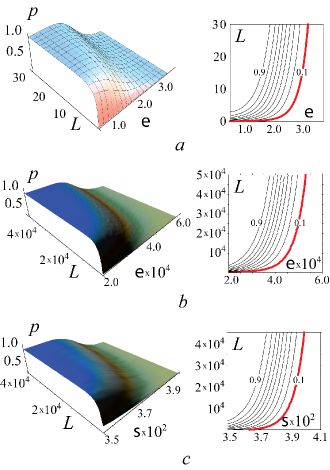
Figure 6: The surface of probability to detect the turbulent phase in the time realization of the system during the observation interval with the length $L$ and corresponding to it the level curves with the step $\Delta P=0.1$. The level curves $P_{b}=0.1$ demarcating the regions with the high and low probabilities to detect the turbulent phase are shown by solid lines. (a) The theoretical expression (19), for the simplicity the values of the control parameters in Eq. (2) are taken $D=1$, $k=1$, $\varepsilon_{c}=0$. (b) The probability surface $P(L,\varepsilon)$ for the circle map with noise (21). (c) The probability surface $P(L,\varepsilon)$ for two coupled Rössler systems (13)

The surface $P(L,\varepsilon)$ determined by the analytical expression (19) and level curves corresponding to it are shown in Fig. 6,a. It is clear that the probability to detect the turbulent phase for type-I intermittency with noise during one observation grows with the increase of the examination length $L$ but decreases when the criticality parameter ${\varepsilon-\varepsilon_{c}}$ is enlarged. Obviously, if one examines (experimentally or numerically) the system behavior in the time interval with the length $L$ varying the control parameter $\varepsilon$, one observes the alternation of the laminar and turbulent phases for the relatively small values of the $\varepsilon$-parameter, where $P(L,\varepsilon)$ is close to one, and only the laminar behavior for the relatively large ones, where $P(L,\varepsilon)$ is close to zero. Having no information about the kind of intermittency (e.g., when the experimental study of some system is carried out) one can suppose the presence of the boundary separating two different types (intermittent and steady) of dynamics and, moreover, find a value $\varepsilon_{2}$ corresponding to the “onset” of the laminar behavior. Evidently, this “boundary point” would be correspond to the low probability $P(L,\varepsilon)$, say, e.g. $P_{b}=P(L,\varepsilon)=0.1$. In addition, one can perform “more careful” measurements with the increased length $L^{\prime}$ of the observation to determine the value of the boundary point $\varepsilon_{2}$ more precisely. In this case a new value $\varepsilon_{2}(L^{\prime})$ would be obtained (${P(L^{\prime},\varepsilon_{2}(L^{\prime}))\approx P_{b}}$), with it being slightly larger than the previous one. The schematic location of the “boundary” curve $\varepsilon_{2}(L)$ on the plane $(\varepsilon,L)$ is shown in Fig. 6,a by the solid line. It is clearly seen, that for the $P_{b}$-level the length $L$ grows extremely rapidly with the increase of the $\varepsilon$-value. In other words, the major extensions of the observation interval $L$ result in the minor corrections of the “boundary” point $\varepsilon_{2}$. Since the resources of the both experimental and numerical studies are always limited, some final value $\varepsilon_{2}$ with the maximal possible accuracy will be eventually found. So, despite the fact, that for the type-I intermittency with noise in the supercritical region the turbulent phases can always be observed theoretically, from the practical point of view (in the experimental studies or numerical calculations) the boundary point $\varepsilon_{2}$ exists, above which only the laminar behavior is observed. Moreover, with the further development of the experimental and computational resources the additional studies would result only in the insufficient increase of the boundary value.

To illustrate the drawn conclusion we consider the circle map

$$x_{n+1}=x_{n}+2\Omega(1-\cos x_{n})-\varepsilon+\xi_{n},\qquad\mathrm{mod}~{}2\pi$$ (20)

in the interval $x\in[-\pi,\pi)$, where $\varepsilon$ is the control parameter, $\Omega=1.0$, $\xi_{n}$ is supposed to be a delta-correlated Gaussian white noise [${\langle\xi_{n}\rangle=0}$, ${\langle\xi_{n}\xi_{m}\rangle=D\delta(n-m)}$]. If the intensity of noise $D$ is equal to zero, the saddle-node bifurcation is observed in (20) for $\varepsilon=\varepsilon_{c}=0$, when the stable and unstable fixed points annihilate at $x=0$. Obviously, for the selected value of the control parameter $\Omega$ the evolution of system (20) in the vicinity of the bifurcation point may be reduced to the quadratic map

$$x_{n+1}=x^{2}_{n}+\frac{1}{4}-\varepsilon+\xi_{n},$$ (21)

allowing an easy comparison with the results given in the previous sections.

The intermittent behavior of type-I is observed for ${\varepsilon<0}$, whereas the stable fixed point takes place for ${\varepsilon>0}$. For the added stochastic force (${D=4\times 10^{-6}}$) in circle map (20) the intermittent behavior is also observed in the supercritical region of the criticality parameter $\varepsilon$, with the mean length $T$ of the laminar phases and the distribution $p(\tau)$ of the laminar phase lengths $\tau$ obeying laws (4) and (5), respectively.

The surface of the probability $P(L,\varepsilon)$ to observe the turbulent phase for the circle map (20) as well as the corresponding level curves are shown in Fig. 6,b. To obtain this surface we have made ${N=2.5\times 10^{4}}$ observations for every point taken with the steps $\Delta L=2\times 10^{2}$, $\Delta\varepsilon=10^{-5}$ on the parameter plane $(\varepsilon,L)$. The probability $P(L,\varepsilon)$ was calculated as ${P(L,\varepsilon)=N_{1}(L,\varepsilon)/N}$, where $N_{1}(L,\varepsilon)$ is the number of observations for which the turbulent phase has been detected. One can see the excellent agreement between the results of numerical calculations and theoretical predictions (compare Fig. 6,a and b).

Similarly, the analogous probability surface $P(L,\sigma)$ and the level curves shown in Fig. 6,c have been calculated for two coupled Rössler systems (13) in the vicinity of the phase synchronization boundary, where eyelet intermittency is observed. In this case $N=10^{3}$ observations have been made for every point to be examined, with these points being taken with the steps $\Delta L=10^{4}$ and $\Delta\sigma=10^{-3}$ on the plane ${(\sigma,L)}$. It is easy to see that for the eyelet intermittency the probability surface as well as the level curves are exactly the same as for type-I intermittency with noise in the supercritical region. As a consequence, we can draw a conclusion, that the eyelet intermittency taking place in the vicinity of the phase synchronization boundary and type-I intermittency with noise in the supercritical region are the same type of the dynamics observed under different conditions. Another consequence of the made consideration is the fact, that the phase synchronization boundary point can not be found absolutely exactly, since it separates the regions with the high and low probabilities to observe the phase slips in the coupled chaotic systems with the help of the experimental and computational resources existing at the moment of study. If someone, using a more powerful tools, tried to refine, say, the value of the coupling strength corresponding to the phase synchronization boundary reported in the earlier paper, one would obtain a new value being close to the previous one, but larger. Exactly the same situation may be found, e.g., in the work [21], where two mutually coupled Rössler systems have been considered. In this work the refined boundary value $\varepsilon_{PS}=0.0416$ is reported with the reference to the earlier work [22], where the value $\varepsilon_{PS}=0.036$ was given.

5 Conclusions

Having considered two types of the intermittent behavior, namely eyelet intermittency taking place in the vicinity of the phase synchronization boundary and type-I intermittency with noise, supposed hitherto to be different, we have shown that these effects are the same type of the dynamics observed under different conditions. The analytical relation between coefficients of the theoretical equations corresponding to both types of the intermittent behavior has been obtained.

The difference between these types of the intermittent behavior is only in the character of the external signal. In case of the type-I intermittency the stochastic signal influences on the system, while in the case of eyelet intermittency the signal of chaotic dynamical system is used to drive the response chaotic oscillator. At the same time, the core mechanism governed the system behavior as well as the characteristics of the system dynamics are the same in both cases.

References

- [1] P. Bergé, Y. Pomeau, C. Vidal, L’Ordre Dans Le Chaos, Hermann, Paris, 1988.
- [2] M. Dubois, M. Rubio, P. Bergé, Experimental evidence of intermiasttencies associated with a subharmonic bifurcation, Phys. Rev. Lett. 51 (1983) 1446–1449.
- [3] N. Platt, E. A. Spiegel, C. Tresser, On–off intermittency: a mechanism for bursting, Phys. Rev. Lett. 70 (3) (1993) 279–282.
- [4] A. E. Hramov, A. A. Koronovskii, Intermittent generalized synchronization in unidirectionally coupled chaotic oscillators, Europhysics Lett. 70 (2) (2005) 169–175.
- [5] A. S. Pikovsky, G. V. Osipov, M. G. Rosenblum, M. Zaks, J. Kurths, Attractor–repeller collision and eyelet intermittency at the transition to phase synchronization, Phys. Rev. Lett. 79 (1) (1997) 47–50.
- [6] K. J. Lee, Y. Kwak, T. K. Lim, Phase jumps near a phase synchronization transition in systems of two coupled chaotic oscillators, Phys. Rev. Lett. 81 (2) (1998) 321–324.
- [7] S. Boccaletti, E. Allaria, R. Meucci, F. T. Arecchi, Experimental characterization of the transition to phase synchronization of chaotic laser systems, Phys. Rev. Lett. 89 (19) (2002) 194101.
- [8] A. E. Hramov, A. A. Koronovskii, M. K. Kurovskaya, S. Boccaletti, Ring intermittency in coupled chaotic oscillators at the boundary of phase synchronization, Phys. Rev. Lett. 97 (2006) 114101.
- [9] Y. Pomeau, P. Manneville, Inetrmittent transition to turbulence in dissipative dynamical systems, Commun. Math. Phys. 74 (1980) 189.
- [10] J. P. Eckmann, L. Thomas, P. Wittwer, Intermittency in the presence of noise, J. Phys. A: Math. Gen. 14 (1981) 3153–3168.
- [11] W. H. Kye, C. M. Kim, Characteristic relations of type-I intermittency in the presence of noise, Phys. Rev. E 62 (5) (2000) 6304–6307.
- [12] A. E. Hramov, A. A. Koronovskii, M. K. Kurovskaya, A. Ovchinnikov, S. Boccaletti, Length distribution of laminar phases for type-I intermittency in the presence of noise, Phys. Rev. E 76 (2) (2007) 026206.
- [13] A. E. Hramov, A. A. Koronovskii, M. K. Kurovskaya, Zero Lyapunov exponent in the vicinity of the saddle-node bifurcation point in the presence of noise, Phys. Rev. E 78 (2008) 036212.
- [14] E. Rosa, E. Ott, M. H. Hess, Transition to phase synchronization of chaos, Phys. Rev. Lett. 80 (8) (1998) 1642–1645.
- [15] C. Grebogi, E. Ott, J. A. Yorke, Fractal basin boundaries, long lived chaotic trancients, and unstable–unstable pair bifurcation, Phys. Rev. Lett. 50 (13) (1983) 935–938.
- [16] A. E. Hramov, A. A. Koronovskii, M. K. Kurovskaya, Two types of phase synchronization destruction, Phys. Rev. E 75 (3) (2007) 036205.
- [17] M. K. Kurovskaya, Distribution of laminar phases at eyelet-type intermittency, Technical Physics Letters 34 (12) (2008) 1063–1065.
- [18] A. E. Hramov, A. A. Koronovskii, Generalized synchronization: a modified system approach, Phys. Rev. E 71 (6) (2005) 067201.
- [19] A. E. Hramov, A. A. Koronovskii, O. I. Moskalenko, Generalized synchronization onset, Europhysics Letters 72 (6) (2005) 901–907.
- [20] O. I. Moskalenko, Transition to phase synchronization in a system with periodic dynamics under the action of a chaotic signal, Technical Physics Letters 33 (10) (2007) 841–843.
- [21] D. Pazó, M. Zaks, J. Kurths, Role of unstable periodic orbits in phase and lag synchronization between coupled chaotic oscillators, Chaos 13 (2002) 309–318.
- [22] M. G. Rosenblum, A. S. Pikovsky, J. Kurths, From phase to lag synchronization in coupled chaotic oscillators, Phys. Rev. Lett. 78 (22) (1997) 4193–4196.