Synchronization in networks of slightly nonidentical elements

Abstract

We study synchronization processes in networks of slightly non identical chaotic systems, for which a complete invariant synchronization manifold does not rigorously exist. We show and quantify how a slightly dispersed distribution in parameters can be properly modelled by a noise term affecting the stability of the synchronous invariant solution emerging for identical systems when the parameter is set at the mean value of the original distribution.

Complex networks are the prominent candidates to describe sophisticated collaborative dynamics in many areas revmod . Recently, the dynamics of complex networks has been extensively investigated with regard to collective (synchronized) behaviors booksPhaseSynchr , with special emphasis on the interplay between complexity in the overall topology and local dynamical properties of the coupled units. The usual case considered so far is that of networks of identical dynamical systems coupled by means of a complex wiring of connections. In this framework, several studies have shown how to enhance synchronization properties, by properly weighting the strengths of the connection wiring M. Chavez, D.-U. Hwang, A. Amann, H.G.E. Hentschel, S. Boccaletti (2005); D.-U. Hwang, M. Chavez, A. Amann, S. Boccaletti (2005); zhoukurths .

In this paper, we extend the study of synchronization phenomena in complex networks to the case of slightly non identical coupled dynamical systems, i.e. networks whose nodes are represented by dynamical systems each one of them evolving with the same functional form, but with a different, node dependent, value of the control parameters. This is motivated by the fact that such a representation seems a more adequate description of many relevant phenomena occurring in natural systems, where the hypothesis that the evolution in different nodes be identical is very often a too restrictive assumption.

Let us then consider a network of $N$ coupled dynamical systems with slightly mismatched control parameters described by the equations

$$\mathbf{\dot{x}}_{i}=\mathbf{F}(\mathbf{x}_{i},\mathbf{g}_{i})-\sigma\sum\limits_{j=1}^{N}G_{ij}\mathbf{H}[\mathbf{x}_{j}],{\quad}i=1,\dots,N,$$ (1)

where $\mathbf{x}_{i}$ are the state vectors in each network node, $\mathbf{F}$ defines the vector field of the considered systems, $\mathbf{g}_{i}$ are the control parameter vectors, $\mathbf{H}[\cdot]$ is an output function, and $\sigma$ is the coupling strength. $G$ is the Laplacian matrix of the network. As so, it is a symmetric zero row sum matrix, it has a real spectrum of eigenvalues ${\lambda_{1}\leq\dots\leq\lambda_{N}}$, $G_{ij}$ ($i\neq j$) is equal to 1 whenever node $i$ is connected with node $j$ and 0 otherwise, and $G_{ii}=-\sum_{j\neq i}G_{ij}$.

When the considered network consists of identical elements (i.e., $\mathbf{g}_{i}=\mathbf{g}$, $\forall i$) the stability of the synchronous state [$\mathbf{x}_{i}(t)=\mathbf{x}_{s}(t)$, $\forall i$] is known to be determined by the diagonalized linear stability equation L.M. Pecora, T.L. Carroll (1998), yielding $N$ blocks of the form

$$\mathbf{\dot{\zeta}}_{i}=\left[J\mathbf{F}(\mathbf{x}_{s},\mathbf{g})-\sigma\lambda_{i}J\mathbf{H}(\mathbf{x}_{s})\right]\zeta_{i},$$ (2)

where $J$ is the Jacobian operator. The blocks (2) differ from each other only by the eigenvalues ${\lambda_{1}\leq\dots\leq\lambda_{N}}$ of the coupling matrix $G$. Replacing $\sigma\lambda_{i}$ by $\nu$ in equation (2), the behavior of the largest (conditional) Lyapunov exponent $\Lambda$ vs $\nu$ [also called master stability function L.M. Pecora, T.L. Carroll (1998)] completely accounts for linear stability of the synchronized manifold. Indeed, the synchronized state associated with $\lambda_{1}=0$ is stable when all the remaining blocks related with the other eigenvalues $\lambda_{i}$ ($i=2,\dots,N$) of coupling matrix $G$ are characterized by the negative Lyapunov exponents. So, to analyze the stability of the synchronized state $\mathbf{x}_{s}(t)$ in the network (1) only one parametric variational equation

$$\mathbf{\dot{\zeta}}=\left[J\mathbf{F}(\mathbf{x}_{s},\mathbf{g})-\nu J\mathbf{H}(\mathbf{x}_{s})\right]\zeta$$ (3)

should be considered to obtain the dependence of the master stability function $\Lambda$ on the parameter $\nu$. Furthermore, the vector state $\mathbf{x}_{s}(t)$ may be obtained as a solution of the uncoupled equation

$$\mathbf{\dot{x}}_{s}(t)=\mathbf{F}(\mathbf{x}_{s}(t),\mathbf{g}).$$ (4)

It is worth noticing that the master stability function $\Lambda(\nu)$ may be negative for a finite interval of $\nu$-parameter values $I_{st}=(\nu_{1};\nu_{2})$ L.M. Pecora, T.L. Carroll (1998) or for an infinite one ($\nu_{2}=\infty$), depending on the specific choice of the functions $\mathbf{F}$ and $\mathbf{H}$. The stability condition is satisfied if the whole set of eigenvalues $\lambda_{i}$ ($i=2,\dots,N$) multiplied by the same $\sigma$ falls into the stability interval $I_{st}$, i.e., when conditions $\sigma\lambda_{2}>\nu_{1}$ and $\sigma\lambda_{N}<\nu_{2}$ take place simultaneously. The vector functions $\mathbf{F}(\cdot)$ and $\mathbf{H}[\cdot]$ are determining the boundaries $\nu_{1}$ and $\nu_{2}$ of the stability interval $I_{st}$, while the eigenvalue distribution is solely ruled by the topology of the imposed wiring of connections.

Natural systems, however, are modelled by networks that generally consist of elements for which parameters might differ. Therefore, equation (3) cannot be seen as a suitable representation of this case. As soon as the vector $\mathbf{g}_{i}$ depends on $i$, an invariant synchronization manifold $\mathbf{x}_{i}(t)=\mathbf{x}_{s}(t)$, $\forall i$ no longer exists, and therefore the arguments of the master stability function do not rigorously apply. However, it has been numerically verified in Ref. M. Chavez, D.-U. Hwang, A. Amann, H.G.E. Hentschel, S. Boccaletti (2005) that, when the difference in the parameters is limited to a slight mismatch, the synchronization behavior keeps on holding in the synchronization region predicted by the master stability function of the system corresponding to the parameter vector ${\mathbf{g}=\langle\mathbf{g}_{i}\rangle}$, where $\langle.\rangle$ stays for the ensemble average on the network nodes.

In the following, we will give ground to such a numerical evidence, and show that, unless a rigorous treatment of the complete synchronization state is prevented, an approximate treatment of these synchronization phenomena is possible under the assumption of a smallness in the parameter mismatch. Without lack of generality, we will develop our points with respect to a subclass of chaotic systems, namely the class of functions $\mathbf{F}$ describing self sustained chaotic oscillators.

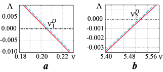
Figure 1: (Color online) The fragments of master stability function corresponding to those $\nu$ ranges for which $\Lambda(\nu)$ crosses the horizontal axis. In both plots a) and b), the dashed line refers to $\Lambda^{D}(\nu)$ calculated for the network of Rössler oscillators with slightly different parameters $\omega_{i}$ at $D=3.5$ (see text for details), whereas the solid line depicts $\Lambda(\nu)$ calculated for the network of identical Rössler oscillators with $\omega_{i}\equiv\bar{\omega}=1$.

The core idea that justifies our approximation comes from the well known property A. Pikovsky, M. Rosenblum, J. Kurths (2001) of a pair of coupled identical chaotic oscillators, where there are two important values ${\sigma_{1}<\sigma_{2}}$ of the coupling strength $\sigma$ determining the transition to complete synchronization. Precisely, $\sigma_{1}$ determines the blowout bifurcation Y. Nagai, Y.-C. Lai (1997); P. Ashwin and E. Stone (1997); Ying-Cheng Lai (1997), when the largest tangential Lyapunov exponent crosses zero. The second one, $\sigma_{2}$ corresponds to the loss of the stability in the tangential direction of the unstable periodic orbits with the lowest period embedded into the synchronized chaotic manifold. When the coupling parameter value is in the interval $\sigma_{1}<\sigma<\sigma_{2}$ the bubbling phenomenon S.C. Venkataramani, B.R. Hunt, E. Ott (1996); S.C. Venkataramani, B.R. Hunt, E. Ott, D.J. Gauthier, and J.C. Bienfang (1996) may be observed. If one considers two coupled identical oscillators the synchronous regime is detected (after expiration of the transient) for coupling strength values $\sigma>\sigma_{1}$. Alternatively, if the control parameters of the coupled oscillators differ slightly from each other, the synchronous behavior may be detected for the coupling strength values exceeding the threshold $\sigma_{2}$. The same effect takes place if two identical oscillators in the presence of noise are considered A. Pikovsky, M. Rosenblum, J. Kurths (2001). In both cases the onset of synchronization is shifted towards the larger values of coupling strength $\sigma$ and determined by the $\sigma_{2}$-value.

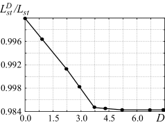
Figure 2: The dependence of the length $L_{st}^{D}$ of the stability interval $I_{st}^{D}$ on the noise intensity $D$ for the network of Rössler oscillators with slightly detuned parameter $\omega_{i}$. The value $L^{D}_{st}$ is normalized on the length $L_{st}$ of the stability interval $I_{st}$ for the network consisting of the identical Rössler oscillators

The idea here is that the property for synchronization of the network consisting of elements with slightly mismatched control parameters $\mathbf{g}_{i}$ may be estimated by means of the consideration of the network of identical elements with the control parameter ${\mathbf{g}=\langle\mathbf{g}_{i}\rangle}$ in the presence of noise. In practice, this assumption means that one can still evaluate the conditional Lyapunov exponents by means of equation (3) at ${\mathbf{g}=\langle\mathbf{g}_{i}\rangle}$, but the evolution of the state $\mathbf{x}_{s}(t)$ around which the conditional exponents are evaluated has to be taken as a solution of a stochastic differential equation, i.e. the evolution equation (4) has to be replaced by

$$\mathbf{\dot{x}}_{s}(t)=\mathbf{F}(\mathbf{x}_{s}(t))+D\mathbf{\xi}(t),$$ (5)

where $D\mathbf{\xi}(t)$ is a noise term with zero mean value.

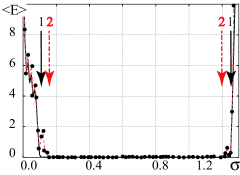
Figure 3: (Color online) $\langle E\rangle$ (see text for definition) vs $\sigma$ for the network of Rössler oscillators with identical parameters $\omega_{i}\equiv\omega=1$ (black solid line) and for the network of Rössler oscillators with slightly detuned parameters $\Delta\omega_{i}=0.07$ (red dashed line with black circles). The arrows labelled with “1” delimit the interval of coupling parameter $\sigma$ for which the error goes to zero in the case of identical oscillators, while the arrows labelled with “2” delimit the interval of $\sigma$ for which the error goes to zero when the oscillators have slightly detuned parameters.

The new stability interval ${I^{D}_{st}=(\nu_{1}^{D},\nu_{2}^{D})}$ for the selected intensity $D$ of noise may be found in the same way as it has been described above by means of calculating the master stability function $\Lambda^{D}(\nu)$. We will show that, under such an assumption, the increase of the noise intensity $D$ leads the boundaries $\nu_{1}^{D}$ and $\nu_{2}^{D}$ of the stability interval $I^{D}_{st}$ to converge to asymptotic values $\nu_{1}^{*}$ and $\nu_{2}^{*}$, respectively. These points $\nu_{1,2}^{*}$ are analogous to the coupling strength value $\sigma_{2}$ in the case of two coupled chaotic oscillators and determine the stability interval $I_{st}^{*}$ for the considered network of slightly non identical elements.

To illustrate the proposed approach let us consider a network of coupled Rössler systems. The dynamics of such network is described by equation (1) with ${\mathbf{x}_{i}=(x_{i},y_{i},z_{i})}$, $\mathbf{g}_{i}=(\omega_{i})$, $\mathbf{F}(\mathbf{x}_{i},\mathbf{g}_{i})=\mathbf{F}(\mathbf{x}_{i},\omega_{i})=[-\omega_{i}y_{i}-z_{i},\omega_{i}x_{i}+0.165y_{i},0.2+z_{i}(x_{i}-10)]$, $\mathbf{H}[\mathbf{x}]=x$:

$$\begin{array}[]{l}\dot{x}_{i}=-\omega_{i}y_{i}-z_{i}-\sigma\sum_{j=1}^{N}G_{ij}x_{j},\\ \dot{y}_{i}=\omega_{i}x_{i}+0.165y_{i},\\ \dot{z}_{i}=0.2+z_{i}(x_{i}-10).\end{array}$$ (6)

The mismatch in the parameters here corresponds to a detuning in the natural frequencies $\omega_{i}$ of the oscillators, that are supposed to be distributed randomly with a mean value $\bar{\omega}=\langle\omega_{i}\rangle=1$ and a small dispersion $\Delta\omega\cong 0.1$.

For the case of identical Rössler oscillators (i.e. assuming all oscillators to have the same natural frequency $\bar{\omega}=1$), it exists a finite range of values for the parameter $\nu$ (that we will call the stability interval $I_{st}$) for which the master stability function is negative L.M. Pecora, T.L. Carroll (1998).

To take into account the small difference in the frequencies of the coupled oscillators, equations (3) and (5) are instead used to calculate the stability interval $I_{st}^{D}$ as discussed above. To calculate the master stability function $\Lambda^{D}(\nu)$ characterizing the property for synchronization of the network with slightly detuned elements, we made use of a random process $\mathbf{\xi}(t)$ distributed uniformly over the interval $(-1.0;1.0)$. To integrate equation (5) the one-step method has been applied J. García-Ojalvo, J.M. Sancho (1999) with the time step $\Delta t=10^{-6}$.

The fragments of the dependence $\Lambda^{D}(\nu)$ around the boundary points $\nu_{1,2}$ are shown in Fig. 1. One can see that the influence of noise in (5) results in the shift of the boundary points $\nu_{1,2}^{D}$ and in the consequent reduction of the stability interval $I_{st}^{D}$. Therefore, the range of the coupling strength value $\sigma$ corresponding to the synchronous dynamics of the network of elements with slightly different values of parameters is less in comparison with the analogous network consisting of the identical elements.

The dependence of the normalized length $L_{st}^{D}/L_{st}$ (where ${L^{D}_{st}=\nu_{2}^{D}-\nu_{1}^{D}}$ and ${L_{st}=\nu_{2}-\nu_{1}}$, respectively) of the stability interval $I^{D}_{st}$ on the intensity of noise $D$ is shown in Fig. 2. One can see that, under the increase of the noise intensity $D$, the length of the stability interval $L^{D}_{st}$ converges to the value $L_{st}^{{\color[rgb]{1,0,0}D}*}$ which does not depend practically on $D$-value. At the same time, the boundaries $\nu_{1}^{D}$ and $\nu_{2}^{D}$ of the stability interval $I_{st}^{D}$ converge to the points $\nu_{1}^{*}$ and $\nu_{2}^{*}$, respectively. Therefore, the obtained interval $I_{st}^{*}$ is the region of parameter $\nu$-values corresponding the stable synchronized behavior of the considered network consisting of elements with slightly different parameter values. It is important to note, that the stability interval $I_{st}^{*}$ is found when the noise intensity $D$ is increased step-by-step. At the same time, if the $D$-value used in (5) is too large (e.g., the noise intensity is comparable to the amplitude of oscillations), the dynamics of oscillator may be destroyed completely by noise, and, as a result, the boundary points of the stability region $I_{st}^{*}$ will not be detected correctly. In other words, there is a range of the reasonable values of the noise intensity $D$ corresponding to the behavior of the network with slightly detuned elements.

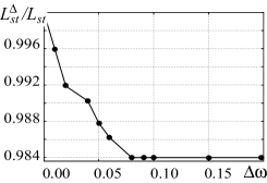
Figure 4: The length $L_{st}^{\Delta}$ of the stability interval $I_{st}^{\Delta}$ vs. the maximum deviation of the control parameter value $\Delta\omega$ for the network of Rössler oscillators with slightly detuned parameters. The value $L^{\Delta}_{st}$ is normalized to that of the length ($L_{st}$) of the stability interval $I_{st}$ for the network consisting of the identical Rössler oscillators.

In order to show that the approximate solution of the master stability formalism is valid already for networks of relatively small size, a direct numerical simulation of Eq. (6) has been carried out for various different values of the control parameters. This calculation allows to find the boundary of the stability of the synchronous regime directly and to compare them with the analogous ones obtained before (based on Equations (3), (5)). We consider here a network of $N=5$ non identical Rössler systems with $\Delta\omega_{i}=0.07$. The coupling matrix $G$ is selected as

$$\left(\begin{array}[]{ccccc}-2&0&0&1&1\\ 0&-3&1&1&1\\ 0&1&-3&1&1\\ 1&0&0&-1&0\\ 1&1&1&0&-3\end{array}\right),$$ (7)

having as eigenvalues $\lambda_{1}=0.0$; $\lambda_{2}\approx-1.6$; $\lambda_{3}\approx-2.0$; $\lambda_{4}\approx-4.0$; $\lambda_{5}\approx-4.4$.

In the simulations, the appearance of a synchronous state can be monitored by looking at the vanishing of the time average (over a window T) synchronization error

$$\langle E\rangle=\frac{1}{T(N-1)}\sum_{j>1}\int^{t+T}_{t}\|\mathbf{x}_{j}-\mathbf{x}_{1}\|dt^{\prime}.$$ (8)

In the present case, we adopt as vector norm $\|\mathbf{x}\|=|x|+|y|+|z|$. Fig. 3 reports the synchronization error versus $\sigma$ for a given network topology. The Figure comparatively reports the case of identical Rössler oscillators all with frequency $\omega=1$, and the case of slightly non identical oscillators with frequencies distributed around the same mean $\bar{\omega}=1$ and with $\Delta\omega=0.07$. One can see that the interval of $\sigma$ for which the error goes to zero reduces in this case, in accordance with the arguments extracted from the Master Stability Function description.

A relevant issue concerns the possibility of establishing a quantitative correspondence between the noise intensity $D$ in equation (5) and the dispersion of the control parameter values in (6). To clarify this point, we consider the ratio $L_{st}^{D}/L_{st}$ between the length of the stability interval for non identical elements in the presence of noise and the same length for the case of identical systems. For the network of elements with the slightly nonidentical control parameters  (6), the stability interval $I^{\Delta}_{st}$ may be defined as the coupling strength range where the synchronization error (8) vanishes.

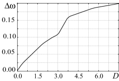
Figure 5: The noise intensity $D$ vs. the control parameter deviation $\Delta\omega$.

The dependence of the normalized length $L_{st}^{\Delta}/L_{st}$ of the stability interval $I^{\Delta}_{st}$ with the value of the maximal deviation $\Delta\omega$ is shown in Fig. 4. By comparison with Fig. 2, it is apparent how the curve in Fig.  4 is in excellent agreement with its analogue depicting the dependence of the normalized length $L_{st}^{D}/L_{st}$ on the noise intensity $D$. Notice that, as the the nonidentity of the network elements ($\Delta\omega$) increases, the length $L_{st}^{\Delta}$ strives for its asymptotic value $L_{st}^{\Delta*}$, which now does not depend on the specific $\Delta\omega$-value. Moreover, this limit value $L_{st}^{\Delta*}$ is in the good concordance with $L_{st}^{D*}$. Finally, in Fig. 5 the relationship between the noise intensity $D$ and the control parameter deviation $\Delta\omega$ is reported, showing that the network of non-identical oscillators can be suitably modelled by a noise addition to the synchronization manifold characterizing the evolution of the corresponding network of identical units.

In conclusion, we have estimated the property for synchronization of networks consisting of equal elements with slightly different control parameter values. This study may be considered as the extension of the already known method of analysis of the behavior of the networks of identical elements.

This work has been supported by Russian Foundation of Basic Research (projects 05–02–16273, 06–02–16451, 06–02–81013). S.B. acknowledges support from the Horovitz Center for Complexity. We also thank the “Dynasty” Foundation.

References

- (1) R. Albert and A. L. Barabási, Rev. Mod. Phys. 74, 47 (2002); S. Boccaletti, V. Latora, Y. Moreno, M. Chavez and D.-U. Hwang, Phys. Rep. 466, 175 (2006).
- (2) S. Boccaletti, J. Kurths, G. Osipov, D.L. Valladares and C.S. Zhou, Phys. Rep. 366, 1 (2002).
- M. Chavez, D.-U. Hwang, A. Amann, H.G.E. Hentschel, S. Boccaletti (2005) M. Chavez, D.-U. Hwang, A. Amann, H.G.E. Hentschel, S. Boccaletti, Phys. Rev. Lett. 94, 218701 (2005).
- D.-U. Hwang, M. Chavez, A. Amann, S. Boccaletti (2005) D.-U. Hwang, M. Chavez, A. Amann, S. Boccaletti, Phys. Rev. Lett. 94, 138701 (2005).
- (5) A. E. Motter, C. Zhou and J. Kurths, Europhys. Lett. 69, 334 (2005), Phys. Rev. E 71, 016116 (2005); C. Zhou, A. E. Motter and J. Kurths, Phys. Rev. Lett. 96, 034101 (2006).
- L.M. Pecora, T.L. Carroll (1998) L.M. Pecora, T.L. Carroll, Phys. Rev. Lett. 80, 2109 (1998).
- A. Pikovsky, M. Rosenblum, J. Kurths (2001) A. Pikovsky, M. Rosenblum, J. Kurths, Synchronization: a universal concept in nonlinear sciences (Cambridge University Press, 2001).
- Y. Nagai, Y.-C. Lai (1997) Y. Nagai, Y.-C. Lai, Phys. Rev. E 55, R1251 (1997).
- P. Ashwin and E. Stone (1997) P. Ashwin and E. Stone, Phys. Rev. E 56, 1635 (1997).
- Ying-Cheng Lai (1997) Ying-Cheng Lai, Phys. Rev. E 56, 1407 (1997).
- S.C. Venkataramani, B.R. Hunt, E. Ott (1996) S.C. Venkataramani, B.R. Hunt, E. Ott, Phys. Rev. E 54, 1346 (1996).
- S.C. Venkataramani, B.R. Hunt, E. Ott, D.J. Gauthier, and J.C. Bienfang (1996) S.C. Venkataramani, B.R. Hunt, E. Ott, D.J. Gauthier, and J.C. Bienfang, Phys. Rev. Lett. 77, 5361 (1996).
- J. García-Ojalvo, J.M. Sancho (1999) J. García-Ojalvo, J.M. Sancho, Noise in Spatially Extended Systems (New York: Springer, 1999).