FIRST EXPERIMENTAL OBSERVATION OF GENERALIZED SYNCHRONIZATION PHENOMENA IN MICROWAVE OSCILLATORS

Abstract

In this Letter we report for the first time on the experimental observation of the generalized synchronization regime in the microwave electronic systems, namely, in the multicavity klystron generators. A new approach devoted to the generalized synchronization detection has been developed. The experimental observations are in the excellent agreement with the results of numerical simulation. The observed phenomena gives a strong potential for new applications requiring microwave chaotic signals.

Chaotic synchronization is one of the fundamental phenomena, widely studied recently, having both theoretical and applied significance Boccaletti et al. (2002). One of the interesting and intricate types of the synchronous behavior of unidirectionally coupled chaotic oscillators is the generalized synchronization (GS) Abarbanel et al. (1996); Hramov and Koronovskii (2005), which means the presence a functional relation between the dynamics of the drive and response chaotic systems, though this relation may be very complicated and its explicit form cannot be found in most cases. Remarkably, that practically all studies of the generalized synchronization phenomenon deal with the low-dimensional model systems or the low frequency oscillators. Even if generalized synchronization in lasers is studied, the oscillations of the total intensity of the laser output are usually considered whose frequency is in the megahertz range, with the oscillator dynamics being described by the system of the ordinary differential equations Uchida et al. (2003). The more complicated objects with the infinite dimensional phase space (such as spatially extended systems (see, e.g., Hramov et al. (2005a)) or oscillators with the delayed feedback) are considered from the point of view of generalized synchronization rarely, and, practically always, numerically.

In this Letter we report for the first time on the experimental revelation of generalized synchronization in the microwave systems with the infinite dimensional phase space, namely, in the multicavity klystron oscillators with the delayed feedback. Along with the theoretical interest this study is also important from the point of view of the practical purposes of communication, where the microwave range signals are used very widely.

To detect the onset of generalized synchronization in the experiment a new approach being applicable to the microwave systems has been developed. Actually, there are various techniques for detecting the presence of GS between chaotic oscillators, such as the method of nearest neighbors Rulkov et al. (1995) or the auxiliary system approach Abarbanel et al. (1996). It is also possible to calculate the conditional Lyapunov exponents Pyragas (1996) to reveal the generalized synchronization regime. Unfortunately, these approaches are often difficult (or impossible) to implement in the experimental measurements (specifically, in the microwave range), due to the presence of noise and lack of the precisions. Therefore, in this Letter we propose the radically different approach which may deal with the chaotic oscillators of the microwave range to detect experimentally the onset of the generalized synchronization regime. Moreover, as we show below, the developed technique may be also used successfully to detect the onset of the GS regime for a very wide range of dynamical systems outside the microwave electronics.

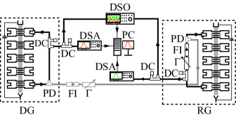
Figure 1: (Color online) The experimental setup for the GS observation in two unidirectionally coupled microwave klystron generators with the delayed feedback. The dashed rectangles correspond to the drive (DG) and response (RG) generators. FI — ferrite isolator; PD — power divider; DC — directional coupler; $\Gamma$ — waveguide attenuator; DSO — digital storage oscilloscope Agilent Technologies DSO81004B; DSA — digital spectrum analyzer Agilent Technologies E4402B; PC — computer. The control parameters of the drive (labeled by “d”) and response (labeled by “r”) oscillators are $V_{0}^{d}=2.1$ kV, $I^{d}=50$ mA, $V_{0}^{r}=1.9$ kV, $I^{r}=52$ mA

Our experimental setup is shown in Fig. 1. We use the S-band five-cavity floating-drift klystron amplifier with the delayed feedback Shigaev et al. (2005) as a drive generator (DG). We can tune the behavior of the generator by changing the acceleration voltage $V_{0}$ and the electron beam current $I_{0}$. The output signal of the drive system with the help of the coaxial line (shown in gray) is transmitted to the input of the response generator (RG), which is analogous to the drive one. To prevent the backward influence of the response klystron oscillator to the drive system we include the ferrite isolator (FI) into the coupling line. The coupling strength between interacting generators may be regulated within wide limits with the help of the attenuators ($\Gamma$). The output microwave signals of both drive [$x(t)$] and response [$y(t)$] generators are measured by the digital storage oscilloscope (DSO) and the digital spectrum analyzer (DSA) and stored in a computer (PC). The typical fragments of time series and power spectra obtained experimentally for the considered klystron generators are shown in Fig. 2.

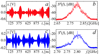
Figure 2: (Color online) The experimentally obtained time series and power spectra. Figures a, b correspond to the drive oscillator and c, d — to the response one. Both oscillators are in the autonomous regime

To detect the onset of the GS regime we propose to analyze the power spectra of chaotic oscillations being one of the important characteristics of the system dynamics. Additionally, they are easily obtained in the experiments. The main idea of the proposed approach is the following. Since the chaotic oscillator dynamics changed sufficiently when GS arises Hramov and Koronovskii (2005), one can expect that this transformation is also manifested in the power spectra modifications. To detect the qualitative changes in the power spectrum of the response system taking place with the increase of the coupling strength ${\varepsilon=10^{-\Gamma/20}}$ (where $\Gamma$ is the attenuation factor of the coupling microwave line) we propose the following characteristic

$$\begin{array}[]{l}\displaystyle{\sigma(\varepsilon)=\frac{1}{P^{d}}\int\limits_{0}^{\infty}\left(\frac{\partial S^{r}(f,\varepsilon)}{\partial\varepsilon}\right)^{2}df},\\ \end{array}$$ (1)

where $P^{d}=\int_{0}^{\infty}S^{d}(f)\,df$ is the total power of the spectrum $S^{d}(f)$ of the drive generator oscillations and $S^{r}(f,\varepsilon)$ — the power spectrum of the response oscillator observed for the coupling strength $\varepsilon$. The derivative $\partial S^{r}(f,\varepsilon)/\partial\varepsilon$ specifies the changes of the power spectra of the response system when the coupling strength $\varepsilon$ is changed. Unless the dynamics of the response system is transformed cardinally the value $\sigma(\varepsilon)$ is not supposed to be changed greatly. Since arising the GS regime means the major restructuring of the response system dynamics Hramov and Koronovskii (2005), one can expect that the noticeable variations in the evolution of the characteristic $\sigma(\varepsilon)$ corresponding to the onset of the GS regime may be observed. Since the power spectra obtained in the experiment are represented by the discrete sets of data, the integral in (1) should be replaced by the sum and, therefore, Eq. (1) takes the form

$$\begin{array}[]{l}\displaystyle{\sigma(\varepsilon)=\frac{1}{\Delta\varepsilon^{2}P^{d}}\sum^{N}_{i=0}\left(\langle S^{r}(f_{i},\varepsilon)\rangle-\langle S^{r}(f_{i},\varepsilon-\Delta\varepsilon)\rangle\right)^{2}},\\ \end{array}$$

where $P^{d}=\sum_{i=1}^{N}\langle(S^{d}(f_{i}))^{2}\rangle$, ${N=2^{12}}$ is the number of the spectral components in the discrete representation of the power spectrum, $\langle\cdot\rangle$ denotes the ensemble average. In the experiment we have used averaging over 512 measurements.

The characteristics $\sigma(\varepsilon)$ obtained from the experiment is shown in Fig. 3. One can see that after the monotonous decrease the curve $\sigma$ vs. $\varepsilon$ shows the pronounced peak ($\varepsilon_{GS}\approx 0.63$) being the manifestation of the great transformation of the response oscillator dynamics. This transformation of the response system behavior is expected to be associated with the onset of the GS regime. Nevertheless, we have to be convinced that the observed peak is really the evidence of the GS regime onset. Note, there is no complete synchronization between oscillators (see correlation plots $y$ vs. $x$ in frames in Fig. 3).

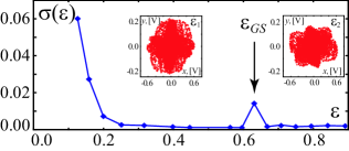
Figure 3: (Color online) The experimental characteristic $\sigma(\varepsilon)$ for two unidirectionally coupled klystron generators. The correlation plots $y$ vs. $x$ are shown in the frames for $\varepsilon_{1}=0.10$ and $\varepsilon_{2}=0.89$, respectively.

To verify the assumption made above, we consider the experimental time series of the drive and response oscillators for two different values of the coupling strength $\varepsilon_{1}=0.10$ and $\varepsilon_{2}=0.89$, below and above the critical value $\varepsilon_{GS}$ supposed to be the boundary of GS. Having selected on different time intervals ${\mathfrak{T}_{1}:t\in[t_{1},t_{1}+T)}$ and ${\mathfrak{T}_{2}:t\in[t_{2},t_{2}+T)}$ (where $T=130$ ns is the time delay of the generator feedback) two nearly identical pieces $x_{1}(\xi)$, $x_{2}(\xi)$ of the drive oscillator time series and corresponding to them two segments $y_{1}(\xi)$, $y_{2}(\xi)$ of the response system time series, we draw the correlation plots $x_{2}$ vs. $x_{1}$ and $y_{2}$ vs. $y_{1}$, respectively (Fig. 4). To detect such similar segments of the drive system time series we consider the distances $d=\int_{0}^{T}(x_{1}(\xi)-x_{2}(\xi))^{2}d\xi$ between two arbitrary pieces $x_{1}$, $x_{2}$ with length $T$ and find the minimal value of $d$. Obviously, if the drive system behavior is practically identical on time intervals $\mathfrak{T}_{1}$ and $\mathfrak{T}_{2}$ (see Fig. 4, a,c), the response system shows also nearly identical dynamics when the GS regime takes place (Fig. 4, d), whereas in the case of absence of GS the behavior of the response oscillator on $\mathfrak{T}_{1}$ and $\mathfrak{T}_{2}$ is different (Fig. 4, b).

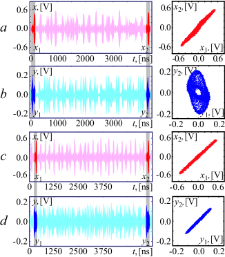
Figure 4: (Color online) The selected fragments of time series and corresponding to them correlation plots. Figures a (drive) and b (response) correspond to the coupling strength $\varepsilon_{1}=0.10$, whereas c (drive) and d (response) — to the coupling strength $\varepsilon_{2}=0.89$

In parallel with the experimental study we have also carried out a numerical simulations of a simple model of two unidirectionally coupled klystron generators with the delayed feedback. With the dynamics of the autonomous klystron generator being in accordance with the numerical simulations of this model Shigaev et al. (2005), the qualitative agreement between experimental and numerical results concerning the behavior of two unidirectionally coupled klystron generators with delay is expected to take place, too. The mathematical form of two coupled generator model is the following

$$\begin{array}[]{l}\displaystyle{\dot{F}^{d}_{1}(\tau)+\gamma^{d}{F}^{d}_{1}(\tau)=\gamma^{d}{F}^{d}_{2}(\tau-1)},\\ \displaystyle{\dot{F}^{d}_{2}(\tau)+\gamma^{d}{F}^{d}_{2}(\tau)=-2i\alpha^{d}{e}^{-i\psi}J_{1}(|F^{d}_{1}(\tau)|)\frac{F^{d}_{1}(\tau)}{|F^{d}_{1}(\tau)|}},\\ \displaystyle{\dot{F}^{r}_{1}(\tau)+\gamma^{r}{F}^{r}_{1}(\tau)=\gamma^{r}((1-\varepsilon){F}^{r}_{2}(\tau-1)+\varepsilon{F}^{d}_{2}(\tau))},\\ \displaystyle{\dot{F}^{r}_{2}(\tau)+\gamma^{r}{F}^{r}_{2}(\tau)=-2i\alpha^{r}{e}^{-i\psi}J_{1}(|F^{r}_{1}(\tau)|)\frac{F^{r}_{1}(\tau)}{|F^{r}_{1}(\tau)|}},\\ \end{array}$$ (2)

where indexes “$d$” and “$r$” relate to the drive and response oscillators; $F_{1}$ and $F_{2}$ are the slowly varying dimensionless amplitudes of oscillations in the input and output cavities, respectively; $\tau$ is the normalized time, $\psi$ is the phase shift during propagation along the feedback circuit, $J_{1}$ is a Bessel function of the first kind, $\gamma$ is the loss parameter, $\alpha$ is a beam current, $\varepsilon$ is a coupling strength. The control parameter values are $\alpha^{r}=10.9$, $\alpha^{d}=10.85$, $\psi=-0.5\pi$, $\gamma^{r}=1.0$, $\gamma^{d}=1.0$. For such a choice of the control parameter values, both the drive and response oscillators generate the chaotic signals.

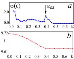
Figure 5: (Color online) (a) The characteristic $\sigma(\varepsilon)$ for two unidirectionally coupled klystron generators (2) and (b) the dependence of the value of the first harmonic of the bunched electron beam current $|I_{1}|$ in the response klystron oscillator on the coupling strength $\varepsilon$. The arrows show the GS onset in coupled microwave oscillators

The character of the evolution of $\sigma$ quantity (Fig. 5, a) is quite similar both for the experiment and numerical model. The peak being analogous to the one of the experimental curve happens to be also observed in the same range of the coupling strength value for the plot $\sigma(\varepsilon)$ obtained by means of numerical simulation of the model system (2) (see Fig. 5, a). Fortunately, the traditional methods of the GS detection mentioned above may be used for the numerical simulation data (contrary to the experimental ones). Based on the auxiliary system approach Abarbanel et al. (1996) we have found that the peak on the curve $\sigma(\varepsilon)$ is certainly the manifestation of the GS onset. Indeed, there is the exact coincidence of the values of coupling strength $\varepsilon$ corresponding to the extremum of the peak of the curve $\sigma(\varepsilon)$ and the onset of GS shown in Fig. 5, a by an arrow. So, the peak on the curve $\sigma(\varepsilon)$ really corresponds to the boundary of the GS regime.

Let us discuss briefly the mechanism of arising the GS regime in a system of unidirectionally coupled klystron oscillators. It is well-known Pyragas (1996); Hramov et al. (2005b) that the proper chaotic dynamics of the response system should be suppressed for the GS regime to take place. The same reason results in arising the GS regime in coupled klystron oscillators. Indeed, the dynamics of the klystron generator is determined by the value of the first harmonic of the bunched electron beam current. In the context of the used model (2) this dimensionless first harmonic of current may be written as $I_{1}=2\alpha^{r}J_{1}\left(|F_{1}(\tau)|/2\right)$.

The dependence of the value of the first harmonic of current on the coupling strength $\varepsilon$ obtained by means of the numerical simulations is shown in Fig. 5, b. One can see that the curve $I_{1}(\varepsilon)$ decreases from the value $I_{1}\approx 9.72$ to $I_{1}\approx 9.61$ when the coupling strength $\varepsilon$ grows, with the sharp decrease corresponding to the GS onset. The generalized synchronization arises when the first harmonic arrives the value $I_{1}\approx 9.61$ (see Fig. 5). Therefore, near the critical value of the coupling strength $\varepsilon_{c}\approx 0.4$ the influence of the drive klystron oscillator results in the decrease of the first harmonic of the current and, correspondingly, in the suppression of the proper chaotic dynamics of the response system, with the GS regime being revealed.

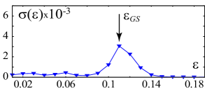
Figure 6: The characteristic $\sigma(\varepsilon)$ obtained from the numerical simulations of unidirectionally coupled Rössler oscillators with the diffusion type of coupling. The control parameters are $a=0.15$, $p=0.2$, $c=10.0$, $w_{r}=0.95$, $w_{d}=0.99$.

There is one more important problem to be considered, namely, whether the proposed GS onset detection technique associated with the characteristic (1) is applicable for a wide range of the different systems. To examine this problem we have studied the dependence of the measure $\sigma(\varepsilon)$ on the coupling strength $\varepsilon$ for two unidirectionally coupled Rössler oscillators

$$\begin{array}[]{ll}\displaystyle{\dot{x}_{d}=-w_{d}y_{d}-z_{d}},&\displaystyle{\dot{x}_{r}=-w_{r}y_{r}-z_{r}+\varepsilon(x_{d}-x_{r})},\\ \displaystyle{\dot{y}_{d}=w_{d}x_{d}+ay_{d}},&\displaystyle{\dot{y}_{r}=w_{r}x_{r}+ay_{r}},\\ \displaystyle{\dot{z}_{d}=p+z_{d}(x_{d}-c)},&\displaystyle{\dot{z}_{r}=p+z_{r}(x_{r}-c)}.\\ \end{array}$$ (3)

In (3) the indexes $``d"$ and $``r"$ relate to the drive and response oscillators, $\varepsilon$ is a coupling strength. The numerically obtained curve $\sigma(\varepsilon)$ is shown in Fig. 6. As well as in the case of two unidirectionally coupled klystron generators there is the pronounced peak in the curves $\sigma(\varepsilon)$ coinciding with the point where the GS regime arises (the onset of GS obtained by means of the auxiliary system approach is shown by an arrow in Fig. 6). The very same results have been obtained for the unidirectionally coupled Rössler and Lorenz oscillators and for the unidirectionally coupled complex Ginzburg-Landau equations (The phenomenon of GS in the coupled Ginzburg-Landau equations was described in Hramov et al. (2005a)). The obtained results provide a basis for expectation that the developed technique can be also applied to bidirectional coupled systems, but this problem deserves a further careful consideration going far beyond the subject of the present Letter.

In conclusion, we have reported on the first experimental observation of the generalized synchronization phenomena in the microwave oscillators with the delayed feedback. We have developed the new techniques of GS determination that can be applied to the experimental study. The proposed techniques have been tested both on experimentally and numerically obtained data. The mechanism of GS arising has been revealed. The experimental observations are in the excellent agreement with the results of numerical simulation. The observed phenomena is supposed to give a strong potential for new applications requiring microwave chaotic signals.

References

- Boccaletti et al. (2002) S. Boccaletti, J. Kurths, G. V. Osipov, D. L. Valladares, and C. T. Zhou, Physics Reports 366, 1 (2002).
- Abarbanel et al. (1996) H. D. Abarbanel, N. F. Rulkov, and M. M. Sushchik, Phys. Rev. E 53, 4528 (1996).
- Hramov and Koronovskii (2005) A. E. Hramov and A. A. Koronovskii, Phys. Rev. E 71, 067201 (2005).
- Uchida et al. (2003) A. Uchida, R. McAllister, R. Meucci, and R. Roy, Phys. Rev. Lett. 91, 174101 (2003).
- Hramov et al. (2005a) A. E. Hramov, A. A. Koronovskii, and P. V. Popov, Phys. Rev. E 72, 037201 (2005a).
- Rulkov et al. (1995) N. F. Rulkov, M. M. Sushchik, L. S. Tsimring, and H. D. Abarbanel, Phys. Rev. E 51, 980 (1995).
- Pyragas (1996) K. Pyragas, Phys. Rev. E 54, R4508 (1996).
- Shigaev et al. (2005) A. M. Shigaev, B. S. Dmitriev, Y. Zharkov, and N. M. Ryskin, IEEE Transactions on Electron Devices 52, 790 (2005).
- Hramov et al. (2005b) A. E. Hramov, A. A. Koronovskii, and O. I. Moskalenko, Europhysics Letters 72, 901 (2005b).