An adaptive POD approximation method for the control of advection-diffusion equations

Abstract.

We present an algorithm for the approximation of a finite horizon optimal control problem for advection-diffusion equations. The method is based on the coupling between an adaptive POD representation of the solution and a Dynamic Programming approximation scheme for the corresponding evolutive Hamilton-Jacobi equation. We discuss several features regarding the adaptivity of the method, the role of error estimate indicators to choose a time subdivision of the problem and the computation of the basis functions. Some test problems are presented to illustrate the method.

1. Introduction

The approximation of optimal control problems for evolutionary partial differential equations of parabolic and hyperbolic type is a very challenging topic with a strong impact on industrial applications. Although there is a large number of papers dealing with several aspects of control problems from controllability to optimal control, the literature dealing with the numerical approximation of such huge problems is rather limited. It is worth to note that when dealing with optimal control problems for parabolic equations we can exploit the regularity of the solutions, regularity which is lacking for many hyperbolic equations. We also recall that the main tools is still given by the Pontryagin maximum principle. This is mainly due to the fact that the discretization of partial differential equations already involves a large number of variables so that the resulting finite dimensional optimization problem easily reaches the limits of what one can really compute. The forward-backward system which describes Pontryagin’s optimality condition is certainly below that limit. However just solving that system one is using necessary conditions for optimality so, in principle, there is no guarantee that these are optimal controls. By this approach for general nonlinear control problems we can obtain just open-loop control. One notable exception is the linear quadratic regulator problem for which we have a closed-loop solution given by the Riccati equation. This explains why the most popular example for the control of evolutive partial differential equations is the control of the heat equation subject to a quadratic cost functional.
In recent years, new tools have been developed to deal with optimal control problems in infinite dimension. In particular, new techniques emerged to reduce the number of dimensions in the description of the dynamical system or, more in general, of the solution of the problem that one is trying to optimize. These methods are generally called reduced-order methods and include for example the POD (Proper Orthogonal Decomposition) method and reduced basis approximation (see [12]). The general idea for all this method is that, when the solution are sufficiently regular, one can represent them via Galerkin expansion so that the number of variables involved in this discretization will be strongly reduced. In some particular case, as for the heat equation, even 5 basis functions will suffice to have a rather accurate POD representation of the solution. Having this in mind, it is reasonable to start thinking to a different approach based on Dynamic Programming (DP) and Hamilton-Jacobi-Bellman equations (HJB). In this new approach we will first develop a reduced basis representation of the solution along a reference trajectory and then use this basis to set-up a control problem in the new space of coordinates. The corresponding Hamilton-Jacobi equation will just need 3-5 variables to represent the state of the system. Moreover, by this method one can obtain optimal control in feedback form looking at the gradient of the value function.
However, the solution of HJB equation it is not an easy task from the numerical point of view: the analytical solution of the HJB equation are non regular (typically, just Lipschitz continuous). Optimal control problems for ODEs were solved by Dynamic Programming, both analytically and numerically (see [1] for a general presentation of this theory). From the numerical point of view, this approach has been developed for many classical control problems obtaining convergence results and a-priori error estimates ([4], [6] and the book [5]). Although this approach suffers from the curse-of-dimensionality some algorithms in high-dimension are now available ([3] and [2]) and the coupling with POD reppresentation techniques will allow to attack by this technique optimal control problems in infinite dimension.
To set this paper into perspective we must say that a first tentative in this direction has been made by Kunisch and co-authors in a series of papers [7, 8] for diffusion dominated equations. In particular, in the paper by Kunisch, Volkwein and Xie [10] one can see a feedback control approach based on coupling between POD basis approximation and HJB equations for the viscous Burgers equation. Our contribution here is twofold. The first novelty is that we deal with advection-diffusion equations. The solutions to these equations exhibit low regularity properties with respect to non degenerate diffusion equations so that a rather large number of POD basis functions will be required to obtain a good approximation if we want to compute the POD basis just once. Naturally, this increases the number of variable in the HJB approach and constitutes a is a real bottle-neck. In order to apply the Dynamic Programming approach to this problem we have developed an adaptive technique which allows to recompute the POD basis on different sub-intervals in order to have always accurate results without an increase of the number of basis functions. The second contribution of this paper is the way the sub-intervals are determined. In fact, we do not use a simple uniform subdivision but rather decide to recompute the POD basis when an error indicator (detailed in Section 4) is beyond a given threshold. As we will show in the sequel, this procedure seems to be rather efficient and accurate to deal with these large scale problems.

2. The POD approximation method for evolutive PDEs

We briefly describe some important features of the POD approximation, more details as well as precise results can be found in the notes by Volkwein [14]. Let us consider a matrix $Y\in\mathbb{R}^{m\times n},$ with rank $d\leq\min\{m,n\}.$ We will call $y_{j}$ the $j-$th column of the matrix $Y.$ We are looking for an orthonormal basis $\{\psi_{i}\}_{i=1}^{\ell}\in\mathbb{R}^{m}$ with $\ell\leq n$ such that the minimum of the following functional is reached:

$$J(\psi_{1},\ldots,\psi_{\ell})=\sum_{j=1}^{n}\left\|y_{j}-\sum_{i=1}^{\ell}\langle y_{j},\psi_{i}\rangle\psi_{i}\right\|^{2}.$$ (2.1)

The solution of this minimization problem is given in the following theorem

Theorem 1.

Let $Y=[y_{1},\ldots,y_{n}]\in\mathbb{R}^{m\times n}$ be a given matrix with rank $d\leq\min\{m,n\}.$ Further, let $Y=\Psi\Sigma V^{T}$ be the Singular Value Decomposition (SVD) of $Y$, where $\Psi=[\psi_{1},\ldots,\psi_{m}]\in\mathbb{R}^{m\times m}$, $V=[v_{1},\ldots,v_{n}]\in\mathbb{R}^{n\times n}$ are orthogonal matrices and the matrix $\Sigma\in\mathbb{R}^{m\times n}$ is diagonal, $\Sigma=diag\{\sigma_{1},\dots,\sigma_{m}\}$. Then, for any $\ell\in\{1,\ldots,d\}$ the solution to (2.1) is given by the left singular vectors $\{\psi_{i}\}_{i=1}^{\ell}$, i.e, by the first $\ell$ columns of $\Psi$.

We will call the vectors $\{\psi_{i}\}_{i=1}^{\ell}$ POD basis of rank $\ell.$ This idea is really usefull, in fact we get a solution solving an equation whose dimension is decreased with respect to the initial one. Whenever it’s possible to compute a POD basis of rank $\ell,$ we get a problem with much smaller dimension of the starting one due to the fact $\ell$ is properly chosen very small.
Let us consider the following ODEs system

$$\left\{\begin{array}[]{ll}\dot{y}(s)=Ay(s)+f(s,y(s)),\;s\in(0,T]\\ \\ y(0)=y_{0}\end{array}\right.$$ (2.2)

where $y_{0}\in\mathbb{R}^{m},A\in\mathbb{R}^{m\times m}$ and $f:[0,T]\times\mathbb{R}^{m}\rightarrow\mathbb{R}^{m}$ is continuous and locally Lipschitz to ensure uniqueness.
The system (2.2) can be also interpreted as a semidiscrete problem, where the matrix $A$ represents the discretization in space of an elliptic operator, say Laplacian for instance. To compute the POD basis functions, first of all we have to construct a time grid $0\leq t_{1}\leq\ldots\leq t_{n}=T$ and we suppose to know the solution of (2.2) at given time $t_{j}$, $j=1,\dots,N$. We call snapshots the solution at those fixed times. For the moment we will not deal with the problem of selecting the snapshots sequence which is a difficult problem in itself, we refer the interested readers to [9]). As soon as we get the snapshots sequence, by Theorem 1, we will be able to compute our POD basis, namely, $\{\psi_{j}\}_{j=1}^{\ell}$.
Let us suppose we can write the solution in reduced form as

$$y^{\ell}(s)=\sum_{j=1}^{\ell}y_{j}^{\ell}(s)\psi_{j}=\sum_{j=1}^{\ell}\langle y^{\ell}(s),\psi_{j}\rangle\psi_{j},\qquad\forall s\in[0,T]$$

substituting this formula into (2.2) we obtain the reduced dynamics

$$\left\{\begin{array}[]{ll}\sum\limits_{j=1}^{\ell}\dot{y}_{j}^{\ell}(s)\psi_{j}=\sum\limits_{j=1}^{\ell}y_{j}^{\ell}(s)A\psi_{j}+f(s,y^{\ell}(s)),\qquad s\in(0,T]\\ \\ \sum\limits_{j=1}^{\ell}y_{j}^{\ell}(0)\psi_{j}=y_{0}.\end{array}\right.$$ (2.3)

We note that our new problem (2.3) is a problem for the $\ell\leq m$ coefficient functions $y_{j}^{\ell}(s),\;j=1,\ldots,\ell.$ Thus, the problem is low dimensional and with compact notation we get:

$$\left\{\begin{array}[]{ll}\dot{y}^{\ell}(s)=A^{\ell}y^{\ell}(s)+F(s,y^{\ell}(s))\\ \\ y^{\ell}(0)=y_{0}^{\ell}\end{array}\right.$$

where

$$A^{\ell}\in\mathbb{R}^{\ell\times\ell}\qquad\mbox{with }(A^{\ell})_{ij}=\langle A\psi_{i},\psi_{j}\rangle,$$

$$y^{\ell}=\left(\begin{array}[]{ccc}y_{1}^{\ell}\\ \vdots\\ y_{\ell}^{\ell}\\ \end{array}\right):[0,T]\rightarrow\mathbb{R}^{\ell}$$

$F=(F_{1},\ldots,F_{\ell})^{T}:[0,T]\times\mathbb{R}^{\ell}\rightarrow\mathbb{R}^{\ell},$

$$F_{i}(s,y)=\left\langle f\left(s,\sum_{j=1}^{\ell}y_{j}\psi_{j}\right),\psi_{i}\right\rangle\;\;\mbox{for }s\in[0,T]\;\;y=(y_{1},\ldots y_{\ell})\in\mathbb{R}^{\ell},$$

finally obtaining the representation of $y_{0}$ in $\mathbb{R}^{\ell}$

$$y_{0}^{\ell}=\left(\begin{array}[]{ccc}\langle y_{0},\psi_{1}\rangle\\ \vdots\\ \langle y_{0},\psi_{\ell}\rangle\\ \end{array}\right)\in\mathbb{R}^{\ell}.$$

In order to apply the POD method to our optimal control problem, the number $\ell$ of POD basis functions is crucial. In particular we would like to keep $\ell$ as low as possible still capturing the behaviour of the original dynamics. The problem is to define an indicator of the accuracy of our POD approximation. A good choice for this indicator is the following ratio

$$\mathcal{E}(\ell)=\dfrac{\sum\limits_{i=1}^{\ell}\sigma_{i}}{\sum\limits_{i=1}^{d}\sigma_{i}}.$$ (2.4)

where the $\sigma_{i}$ are the the singular value obtained by the SVD.

As much $\mathcal{E}(\ell)$ is close to one as much our approximation will be improved. This is strictly related to the truncation error due to the projection of $y_{j}$ onto the space generated by the orthonormal basis $\{\psi\}_{i=1}^{\ell},$ in fact:

$$J(\psi_{1},\ldots,\psi_{\ell})=\sum_{j=1}^{n}\left\|y_{j}-\sum_{i=1}^{\ell}\langle y_{j},\psi_{i}\rangle\psi_{i}\right\|^{2}=\sum_{i=\ell+1}^{d}\sigma_{i}^{2}$$

3. An optimal control problem

We will present this approach for the finite horizon control problem. Consider the controlled system

$$\left\{\begin{array}[]{l}\dot{y}(s)=f(y(s),u(s),s),\;\;s\in(t,T]\\ y(t)=x\in\mathbb{R}^{n},\end{array}\right.$$ (3.1)

we will denote by $y:[t,T]\rightarrow\mathbb{R}^{n}$ its the solution, by $u$ the control $u:[t,T]\rightarrow\mathbb{R}^{m}$, $f:\mathbb{R}^{n}\times\mathbb{R}^{m}\rightarrow\mathbb{R}^{n}$, $s\in(t,T]$ and by

$$\mathcal{U}=\{u:[0,T]\rightarrow U\}$$

the set of admissible controls where $U\subset\mathbb{R}^{m}$ is a compact set. Whenever we want to emphasize the depence of the solution from the control $u$ we will write $y(t;u)$. Assume that there exists a unique solution trajectory for (3.1) provided the controls are measurable (a precise statement can be found in [1]). For the finite horizon optimal control problem the cost functional will be given by

$$\min_{u\in\mathcal{U}}J_{x,t}(u):=\int_{t}^{T}L(y(s,u),u(s),s)e^{-\lambda s}\,ds+g(y(T))$$ (3.2)

where $L:\mathbb{R}^{n}\times\mathbb{R}^{m}\rightarrow\mathbb{R}$ is the running cost and $\lambda\geq 0$ is the discount factor.
The goal is to find a state-feedback control law $u(t)=\Phi(y(t),t),$ in terms of the state equation $y(t),$ where $\Phi$ is the feedback map. To derive optimality conditions we use the well-known dynamic programming principle due to Bellman (see [1]). We first define the value function:

$$v(x,t):=\inf\limits_{u\in\mathcal{U}}J_{x,t}(u)$$ (3.3)

Proposition 3.1 (DPP).

For all $x\in\mathbb{R}^{n}$and $0\leq\tau\leq t$ then:

$$v(x,t)=\min_{u\in\mathcal{U}}\left\{\int_{t}^{\tau}L(y(s),u(s),s)e^{-\lambda s}\;ds+v(y,t-\tau)\right\}.$$ (3.4)

Due to (3.4) we can derive the Hamilton-Jacobi-Bellman equations (HJB):

$$-\dfrac{\partial v}{\partial t}(y,t)=\min_{u\in U}\left\{L(y,u,t)+\nabla v(y,t)\cdot f(y,u,t)\right\}.$$ (3.5)

This is nonlinear partial differential equation of the first order which is hard to solve analitically although a general theory of weak solutions is available [1]. Rather we can solve it numerically by means of a finite differences or semi-Lagrangian schemes (see the book [5] for a comprehensive analysis of approximation schemes for Hamilton-Jacobi equations). For a semi-Lagrangian discretization one starts by a discrete version of (HJB) by discretizing the underlined control problem and then project the semi-discrete scheme on a grid obtaining the fully discrete scheme

$$\left\{\begin{array}[]{ll}v_{i}^{n+1}=\min\limits_{u\in U}[\Delta t\,L(x_{i},n\Delta t,u)+I[v^{n}](x_{i}+\Delta t\,F(x_{i},t_{n},u))]\\ \\ v_{i}^{0}=g(x_{i}).\end{array}\right.$$

with $x_{i}=i\Delta x,\;t_{n}=n\Delta t,\;v^{n}_{i}:=v(x_{i},t_{n})$ and $I[\cdot]$ is an interpolation operator which is necessary to compute the value of $v^{n}$ at the point $x_{i}+\Delta t\,F(x_{i},t_{n},u)$ (in general, this point will not be a node of the grid). The interested reader will find in [6] a detailed presentation of the scheme and a priori error estimates for its numerical approximation.

Note that, we also need to compute the minimum in order to get the value $v_{i}^{n+1}$. Since $v^{n}$ is not a smooth function, we compute the minimum by means of a minimization method which does not use derivatives (this can be done by the Brent algorithm as in [3]).

As we already told the HJB allows to compute the optimal feedback via the value function, but there are two major difficulties: the solution of an HJB equation are in general non-smooth and the approximation in high dimension is not feasible. The request to solve an HJB in high dimension comes up naturally whenever we want to control evolutive PDEs. Just to give an idea, if we build a grid in $[0,1]\times[0,1]$ with a discrete step $\Delta x=0.01$ we have $10^{4}$ nodes: to solve an HJB in that dimension is simply impossible. Fortunatelly, the POD method allows us to obtain reduced models even for complex dynamics. Let us focus on the following abstract problem:

$$\left\{\begin{array}[]{ll}\dfrac{d}{ds}\langle y(s),\varphi\rangle_{H}+a(y(s),\varphi)=\langle B(u(s),\varphi\rangle_{V^{\prime},V}\quad\forall\varphi\in V\\ \\ y(t)=y_{0}\;\;\in H,\end{array}\right.$$ (3.6)

where $B:U\rightarrow V^{\prime}$ is a linear and continuous operator. We assume that a space of admissible controls $\mathcal{U}_{ad}$ is given in such a way that for each $u\in\mathcal{U}_{ad}$ and $y_{0}\in H$ there exists a unique solution $y$ of (3.6). $V$ and $H$ are two Hilbert spaces, with $\langle\cdot,\cdot\rangle_{H}$ we denote the scalar product in $H;$ $a:V\times V\rightarrow\mathbb{R}:$ is symmetric coercive and bilinear. Then, we introduce the cost functional of the finite horizon problem

$$\mathcal{J}_{y_{0},t}(u):=\int_{t}^{T}L(y(s),u(s),s)e^{-\lambda s}\;ds+g(y(T)),$$

where $L:V\times U\times[0,T]\rightarrow\mathbb{R}.$ The optimal control problem is

$$\min\limits_{u\in\mathcal{U}_{ad}}\mathcal{J}_{y_{0},t}(u)$$ (3.7)

subject to the constraint: $$y\in W_{loc}(0,T;V)\times\mathcal{U}\hbox{ solves }(\ref{pabs})$$

with $W_{loc}(0,T)=\bigcap_{T>0}W(0,T),$ where $W(0,T)$ is the standard Sobolev space:

$$W(0,T)=\{\varphi\in L^{2}(0,T;V),\varphi_{t}\in L^{2}(0,T;V^{\prime})\}.$$

The model reduction approach for an optimal control problem (3.7) is based on the Galerkin approximation of dynamic with some informations on the controlled dynamic (snapshots). To compute a POD solution for (3.7) we make the following ansatz

$$y^{\ell}(x,s)=\sum_{i=1}^{\ell}w_{i}(s)\psi_{i}(x).$$ (3.8)

where $\{\psi\}_{i=1}^{\ell}$ is the POD basis computed as in the previous section.
We introduce mass and stiffness matrix:

$$M=((m_{ij}))\in\mathbb{R}^{\ell\times\ell}\mbox{ with }m_{ij}=\langle\psi_{j},\psi_{i}\rangle_{H},$$

$$S=((s_{ij}))\in\mathbb{R}^{\ell\times\ell}\mbox{ with }m_{ij}=a(\psi_{j},\psi_{i}),$$

and the control map $b:U\rightarrow\mathbb{R}^{\ell}$ is defined by:

$$u\rightarrow b(u)=(b(u)_{i})\in\mathbb{R}^{\ell}\mbox{ with }b(u)_{i}=\langle Bu,\psi_{i}\rangle_{H}.$$

The coefficients of the initial condition $y^{\ell}(0)\in\mathbb{R}^{\ell}$ are determined by $w_{i}(0)=(w_{0})_{i}=\langle y_{0},\psi\rangle_{X},\;\;1\leq i\leq\ell,$ and the solution of the reduced dynamic problem is denoted by $w^{\ell}(s)\in\mathbb{R}^{\ell}.$ Then, the Galerkin approximation is given by

$$\min J^{\ell}_{w^{\ell}_{0},t}(u)\\$$ (3.9)

with $u\in\mathcal{U}_{ad}$ and $w$ solves the following equation:

$$\left\{\begin{array}[]{ll}\dot{w}^{\ell}(s)=F(w^{\ell}(s),u(s),s)\;\;\;s>0,\\ \\ w^{\ell}(0)=w_{0}^{\ell}.\end{array}\right.$$ (3.10)

The cost functional is defined:

$$J^{\ell}_{w_{0}^{\ell},t}(u)=\int_{0}^{T}L(w^{\ell}(s),u(s),s)e^{-\lambda s}\;dt+g(w^{\ell}(T)),$$

with $w^{\ell}$ and $y^{\ell}$ linked to (3.8) and the nonlinear map $F:\mathbb{R}^{\ell}\times U\rightarrow\mathbb{R}^{\ell}$ is given by

$$F(w^{\ell},u,s)=M^{-1}(-Sw^{\ell}(s)+b(u(s))).$$

The value function $v^{\ell}$, defined for the initial state $w_{0}\in\mathbb{R}^{\ell},$

$$v^{\ell}(w^{\ell}_{0},t)=\inf_{u\in\mathcal{U}_{ad}}J^{\ell}_{w_{0}^{\ell},t}(u)$$

and $w^{\ell}$ solves (3.9) with the control $u$ and initial condition $w_{0}.$

We give an idea how we have computed the intervals for reduced HJB. HJBs are defined in $\mathbb{R}^{n},$ but we have restricted our numerically domain $\Upsilon_{h}$ which is a bounded subset of $\mathbb{R}^{n}.$ This is justified since $y+\Delta tF(y,u)\in\Upsilon_{h}$ for each $y\in\Upsilon_{h}$ and $u\in\mathcal{U}_{ad}.$ We can chose $\Upsilon_{h}=[a_{1},b_{1}]\times[a_{2},b_{2}]\times\ldots[a_{\ell},b_{\ell}]$ with $a_{1}\geq a_{2}\geq\ldots\geq a_{\ell}.$ How should we compute these intervals $[a_{i},b_{i}]$?
Ideally the intervals should be chosen so that the dynamics contains all the components of the controlled trajectory. Moreover, they should be encapsulated because we expect that their importance should decrease monotonically with their index and that our interval lengths decrease quickly.
Let us suppose to discretize the space control $U=\{u_{1},\ldots,u_{M}\}$ where $U$ is symmetric, to be more precise if $\bar{u}\in U\Rightarrow-\bar{u}\in U.$
Hence, if $y^{\ell}(s)=\sum\limits_{i=1}^{\ell}\langle y(s),\psi_{i}\rangle\psi_{i}=\sum_{i=1}^{\ell}w_{i}(s)\psi_{i},$ as a consequence, the coefficients $w_{i}(s)\in[a_{i},b_{i}].$ We consider the trajectories solution $y(s,u_{j})$ such that the control is constant $u(s)\equiv u_{j}$ for each $t_{j}$, $j=1,\ldots,M.$ Then, we have

$$y^{\ell}(s,u_{j})=\sum_{i=1}^{\ell}\langle y(s,u_{j}),\psi_{i}\rangle\psi_{i}.$$

We write $y^{\ell}(s,u_{j})$ to stress the dependence on the constant control $u_{j}.$ Each trajectory $y^{\ell}(s,u_{j})$ has some coefficients $w_{i}^{(j)}(t)$ for $i=1,\ldots,\ell,\,j=1,\ldots,M.$ The coefficients $w_{i}^{(j)}(s)$ will belong to intervals of the type $[\underline{w}_{i}^{(j)},\overline{\rm{w}}_{i}^{(j)}]$ where we chose for $i=1,\ldots,\ell,$ $a_{i},b_{i}$ such that:

$$a_{i}\equiv\min\{\underline{w}_{i}^{(1)},\ldots,\underline{w}_{i}^{(M)}\}$$

$$b_{i}\equiv\max\{\overline{\rm{w}}_{i}^{(1)},\ldots,\overline{\rm{w}}_{i}^{(M)}\}.$$

Then, we have a method to compute the intervals and we turn our attention to the numerical solution of an optimal control problem for evolutive equation, as we will see in the following section.

4. Adapting POD approximation

We now present an adaptive method to compute POD basis. Since our final goal is to obtain the optimal feedback law by means of HJB equations, we will have a big constraint on the number of variables in the state space for numerical solution of an HJB.
We will see that, for a parabolic equation, one can try to solve the problem with only three/four POD basis functions; they are enough to describe the solution in a rather accurate way. In fact the singular values decay pretty soon and it’s easier to work with a really low-rank dimensional problem.
On the contrary, hyperbolic equations do not have this nice property for their singular values and they will require a rather large set of POD basis functions to get accurate results. Note that we can not follow the approach suggested in [13] because we can not add more basis functions when it turns to be necessary due to the constraint already mentioned. Then, it is quite natural to split the problem into subproblems having different POD basis functions. The crucial point is to decide the splitting in order to have the same number of basis functions in each subdomain with a guaranteed accuracy in the approximation.
Let us first give an illustrative example for the parabolic case, considering a 1D advection-diffusion equation:

$$\left\{\begin{array}[]{ll}y_{s}(x,s)-\varepsilon y_{xx}(x,s)+cy_{x}(x,s)=0\\ y(x,0)=y_{0}(x),\end{array}\right.$$ (4.1)

with $x\in[a,b],s\in[0,T],\varepsilon,c\in\mathbb{R}.\\$ We use a finite difference approximation for this equation based on an explicit Euler method in time combined with the standard centered approximation of the second order term and with an up-wind correction for the advection term. The snapshots will be taken from the sequence generated by the finite difference method. The final time is $T=5$, moreover $a=-1$, $b=4$. The initial condition is $y_{0}(x)=5x-5x^{2},$ when $0\leq x\leq 1$, 0 otherwise.
For $\varepsilon=0.05$ and $c=1$ with only 3 POD basis functions, the approximation fails (see Figure 1). Note that in this case the advection is dominating the diffusion, a low number of POD basis functions will not suffice to get an accurate approximation (Figure 1.b). However, the adaptive method which only uses 3 POD basis functions will give accurate results (Figure 1.d).

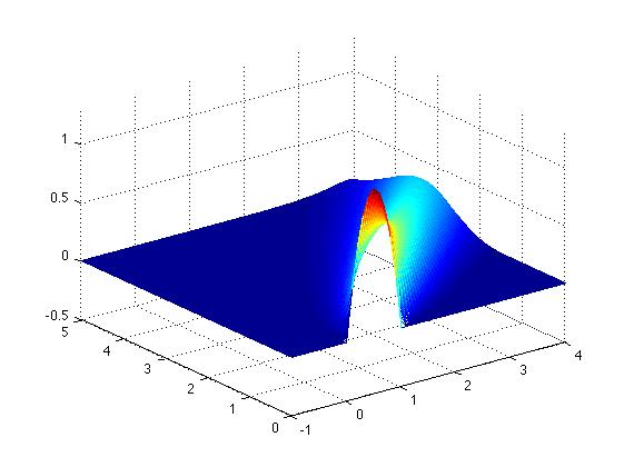
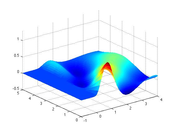
(a)                                               (b)

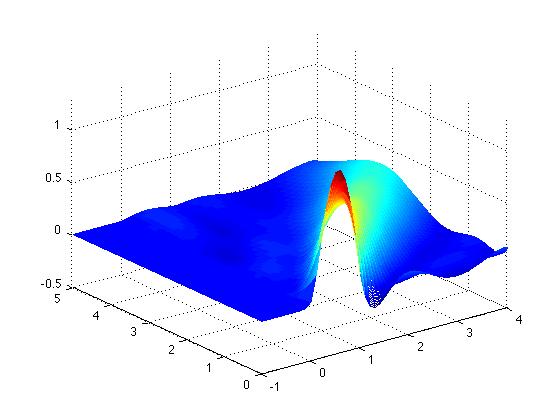
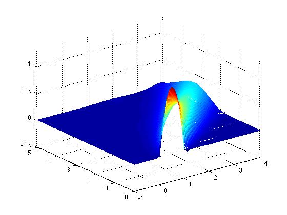
(c)                                               (d)

Figure 1. Equation (4.1):(a) solved with finite difference; (b) POD-Galerkin approximation with 3 POD basi; (c) solved via POD-Galerkin approximation with 5 POD basis; (d) Adapting 3 POD basis functions.

The idea which is behind the adaptive method is the following: we do not consider all the snapshots together in the whole interval $[0,T]$ but we group them. Instead of taking into account the whole interval $[0,T],$ we prefer to split it in sub-intervals

$$[0,T]=\cup_{k=0}^{K}[T_{k},T_{k+1}]$$

where $K$ is a-priori unknown, $T_{0}=0,T_{K}=T$ and $T_{k}=t_{i}$ for some $i.$ In this way, choosing properly the length of the $k-$th interval $[T_{k},T_{k+1}],$ we consider only the snapshots falling in that sub-interval, typically there will be at least three snapshots in every sub-interval. Then we have enough informations in every sub-interval and we can apply the standard routines (explained in Section 2) to get a ”local” POD basis.
Now let us explain how to divide our time interval $[0,T]$. We will choose a parameter to check the accuracy of the POD approximation and define a threshold. Above that threshold we loose in accuracy and we need to compute a new POD basis. A good parameter to check the accuracy is $\mathcal{E}(\ell)$ (see (2.4)), as it was suggested by several authors. The method to define the splitting of $[0,T]$ and the size of every sub-interval works as follows. We start computing the SVD of the matrix $Y$ that gives us informations about our dynamics in the whole time interval. We check the accuracy at every $t_{i}$, $i=1,\dots N$, and if at $t_{k}$ the indicator is above the tolerance we set $T_{1}=t_{k}$ and we divide the interval in two parts, $[0,T_{1})$ and $(T_{1},T]$. Now we just consider the snapshots related the solution up to the time $T_{1}$. Then we iterate this idea until the indicator is below the threshold. When the first interval is found, we restart the procedure in the interval $[T_{1},T]$ and we stop when we reach the final time $T$. Note that the extrema of every interval coincide by construction with one of our discrete times $t_{i}=i\Delta t$ so that the global solution is easily obtained linking all the sub-problems which always have a snapshot as initial condition. A low value for the threshold will also guarantee that we will not have big jumps passing from one sub-interval to the next.

This idea can be applied also when we have a controlled dynamic (see (5.1)). First of all we have to decide how to collect the snapshots, since the control $u(t)$ is completely unknown. One can make a guess and use the dynamics and the functional corresponding to that guess, by these informations we can compute the POD basis. Once the POD basis is obtained we will get the optimal feedback law after having solved a reduced HJB equation as we already explained. Let us summarize the method in the following step-by-step presentation.

ALGORITHM
Start: Inizialization
Step 1: collect the snapshots in [0,T]
Step 2: divide $[0,T]$ according to $\mathcal{E}(\ell)$
For i=0 to N-1
Do
x  Step 3: apply SVD to get the POD basis in each sub-interval $[t_{i},t_{i+1}]$
x  Step 4: discretize the space of controls
x  Step 5: project the dynamics onto the (reduced) POD space
x  Step 6: select the intervals for the POD reduced variables
x  Step 7: solve the corresponding HJB in the reduced space
x         for the interval $[t_{i},t_{i+1}]$
x  Step 8: go back to the original coordinate space
End

5. Numerical experiments

In this section we present some numerical tests for the controlled heat equation and for the advection-diffusion equation with a quadratic cost functional. Consider the following advection-diffusion equation:

$$\left\{\begin{array}[]{ll}y_{s}(x,s)-\varepsilon y_{xx}(x,s)+cy_{x}(x,s)=u(s)\\ y(x,0)=y_{0}(x),\end{array}\right.$$ (5.1)

with $x\in[a,b]$, $s\in[0,T]$, $\varepsilon\in\mathbb{R}_{+}$ and $c\in\mathbb{R}.\\$Note that changing the parameters $c$ and $\varepsilon$ we can obtain the heat equation ($c=0$) and the advection equation ($\varepsilon=0$). The functional to be minimized is

$$J_{y_{0},t}(u(\cdot))=\int_{0}^{T}||y(x,s)-\widehat{y}(x,s)||^{2}+R||u(s)||^{2}\;ds,$$ (5.2)

i.e. we want to stay close to a reference trajectory $\widehat{y}$ while minimizing the norm of $u$. Note that we dropped the discount factor setting $\lambda=0$. Typically in our test problems $\widehat{y}$ is obtained by applying a particular control $\widehat{u}$ to the dynamics. The numerical simulations reported in this papers have been made on a server SUPERMICRO 8045C-3RB with 2 cpu Intel Xeon Quad-Core 2.4 Ghz and 32 GB RAM under SLURM (https://computing.llnl.gov/linux/slurm/).

Test 1: Heat equation with smooth initial data

We compute the snapshots with a centered/forward Euler scheme with space step $\Delta x=0.02$, and time step $\Delta t=0.012$, $\varepsilon=1/60,c=0,R=0.01$ and $T=5$. The initial condition is $y_{0}(x)=5x-5x^{2},$ and $\widehat{y}(x,s)=0.$ In Figure 2 we compare four different approximations concerning the heat equation: (a) is the solution for $\widehat{u}(t)=0$, (b) is its approximation via POD (non adaptive), (c) is the direct LQR solution computed by MATLAB without POD and, finally, the approximate optimal solution obtained coupling POD and HJB. The approximate value function is computed for $\Delta t=0.1$ $\Delta x=0.1$ whereas the optimal trajectory as been obtained with $\Delta t=0.01.$ Test 1, and even Test 2, have been solved in about half an hour of CPU time.
Note that in this example the approximate solution is rather accurate because the regularity of the solution is high due to the diffusion term. Since in the limit the solution tends to the average value the choice of the snapshots will not affect too much the solution, i.e. even with a rough choice of the snapshots will give us a good approximation. The difference between Figure 2c and Figure 2d is due to the fact that the control space is continuous for 2c and discrete for 2d.

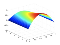
(a)                                               (b)

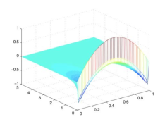
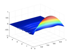
(c)                                               (d)

Figure 2. Test 1:(a) Heat Equation without control; (b) Heat Equation without control, 3 POD basis; (c) Controlled solution with LQR-MATLAB; (d) Approximate solution POD (3 basis functions) + HJB.

Test 2: Heat equation with no-smooth intial data

In this section we change the initial condition with a function which is only Lipschitz continuos: $y_{0}(x)=1-|x|.$ According to Test 1, we consider the same parameters. (see Figure 3).

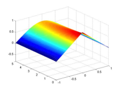
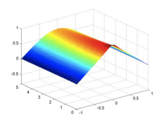
(a)                                               (b)

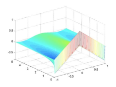
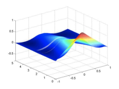
(c)                                               (d)

Figure 3. Test 2: (a) exact solution for $\widehat{u}=0$; (b) Exact solution for $\widehat{u}=0$ POD (3 basis functions); (c) Approximate optimal solution for LQR-MATLAB; (d) Approximate solution POD (3 basis functions)+ HJB.

Riccati’s equation has been solved by a MATLAB LQR routine. Thus, we have used the solution given by this routine as the correct solution in order to compare the errors in $L^{1}$ and $L^{2}$ norm between the reduced Riccati’s equation and our approach based on the reduced HJB equation. Since we do not have any information, the snapshots are computed for $\widehat{u}=0.$ This is only a guess, but in the parabolic case fits well due to the diffusion term.

	$L^{1}$	$L^{2}$
$y^{LQR}-y^{POD+LQR}$	0.0221	0.0172
$y^{LQR}-y^{POD+HJB}$	0.0204	0.0171

Table 1. Test 2: $L^{1}$ and $L^{2}$ errors at time $T$ for the optimal approximate solution.

As in Test 1, the choice of the snapshots does not effect strongly the approximation due to the asymptotic behavior of the solution. The presence of a Lipschitz continuous initial condition has almost no influence on the global error (see Table 1).

Test 3: Advection-Diffusion equation

The advection-diffusion equation needs a different method. We can not use the same $\widehat{y}$ we had in the parabolic case, mainly because in Riccati’s equation the control is free and is not bounded, on the contrary when we solve an HJB we have to discretize the space of controls. We modified the problem in order to deal with bang-bang controls. We get $\widehat{y}$ in (5.2) just plugging in the control $\widehat{u}\equiv 0$. We have considered the control space corresponding only to three values in $[-1,1]$, then $U=\{-1,0,1\}.$ We first have tried to get a controlled solution, without any adaptive method and, as expected, we obtained a bad approximation (see Figure 4).

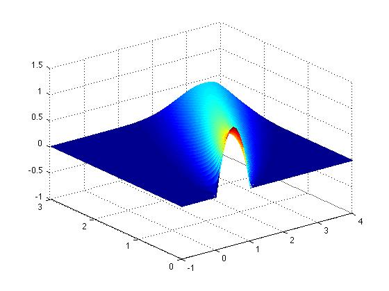
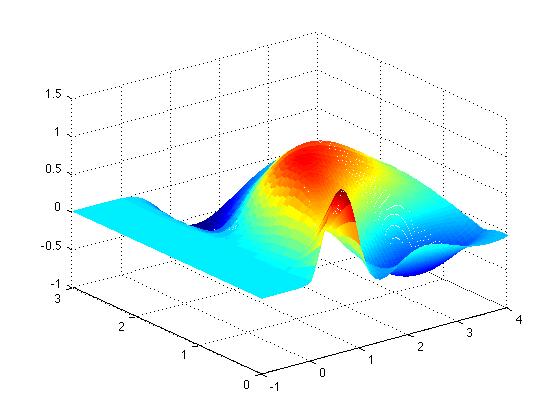
Figure 4. Test 3: Solution $\widehat{y}$ on the left, approximate solution on the right with POD (4 basis functions)

From Figure 4 it’s clear that POD with four basis functions is not able to catch the behavior of the dynamics, so we have applied our adaptive method.

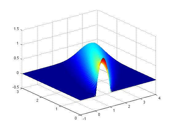
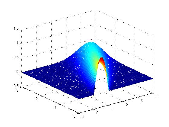
Figure 5. Test 3: Solution for $\widehat{u}\equiv 0$ (left), approximate optimal solution (right).

We have consider: $T=3,\Delta x=0.1,\Delta t=0.008$, $a=-1$, $b=4$, $R=0.01.$ According to our algorithm, the time interval $[0,3]$ was divided into $[0,0.744]\cup[0.744,1.496]\cup[1.496,3].$ As we can see our last interval is bigger than the others, this is due to the diffusion term (see Figure 5). The $L^{2}-$error is 0.0761, and the computation of the optimal solution via HJB has required about six hours of CPU time. In Figure 4 we compare the exact solution with the numerical solution based on a POD representation. Note that, in this case, the choice of only 4 basis functions for the whole interval $[0,T]$ gives a very poor result due to the presence of the advection term. Looking at Figure 5 one can see the improvement of our adaptive technique which takes always 4 basis functions in each sub-interval.
In order to check the quality of our approximation we have computed the numerical residual, defined as:

$$\mathcal{R}(y)=\|y_{s}(x,s)-\varepsilon y_{xx}(x,s)+cy_{x}(x,s)-u(s)\|.$$

The residual for the solution of the control problem computed without our adaptive technique is 1.1, whereas the residual for the adaptive method is $2*10^{-2}$. As expected from the pictures, there is a big difference between these two value.

Test 4: Advection-Diffusion equation

In this test we take a different $\widehat{y}$, namely the solution of (5.1) corresponding to the control

$$\widehat{u}(t)=\left\{\begin{array}[]{l}-1\quad 0\leq t<1\\ 0\quad 1\leq t<2\\ 1\quad 2\leq t\leq 3.\end{array}\right.$$

We want to emphasize we can obtain nice results when the space of controls has few element. The parameters were the same used in Test 3. The $L^{2}-$error is 0.09, and the time was the same we had in Test 3. In Figure 6 we can see our approximation.

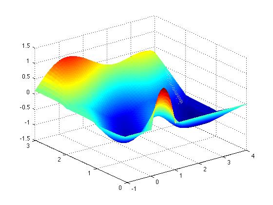
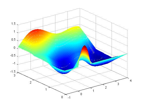
Figure 6. Test 4: Solution for $\widehat{u}$ (left), approximate optimal solution (right).

In Figure 6 one can see that the adaptive technique can also deal with discontinuous controls.

In this test, the residual for the solution of the control problem without our adaptive technique is 2, whereas the residual for the adaptive method is $3*10^{-2}$. Again, the residual shows the higher accuracy of the adaptive routine.

6. Conclusions

As we have discussed, a reasonable coupling between POD and HJB equation can produce feedback controls for infinite dimensional problem. For advection dominated equations that simple idea has to be implemented in a clever way to be successful. It particular, the application of an adaptive technique is crucial to obtain accurate approximations with a low number of POD basis functions. This is still an essential requirement when dealing with the Dynamic Programming approach, which suffers from the curse-of-dimensionality although recent developments in the methods used for HJB equations will allow to increase this bound in the next future (for example by applying patchy techniques).

Another important point is the discretization of the control space. In our examples, the number of optimal control is rather limited and this will be enough for problems which have a bang-bang structure for optimal controls. In general, we will need also an approximation of the control space via reduced basis methods. This point as well as a more detailed analysis of the procedure outlined in this paper will be addressed in our future work.

References

- [1] M. Bardi, I. Capuzzo Dolcetta. Optimal control and viscosity solutions of Hamilton-Jacobi-Bellman equations. Birkhauser, Basel, 1997.
- [2] S. Cacace, E. Cristiani, M. Falcone, A. Picarelli. A patchy dynamic programming scheme for a class of Hamilton-Jacobi-Bellman equations, preprint, 2011 to appear on SIAM J. Sci. Comp.
- [3] E. Carlini, M. Falcone, R. Ferretti. An efficient algorithm for Hamilton-Jacobi equations in high dimension. Computing and Visualization in Science, Vol.7, No.1 (2004) pp. 15-29.
- [4] M. Falcone. Numerical solution of dynamic programming equations, Appendix of the book M. Bardi, I. Capuzzo Dolcetta, Optimal control and viscosity solutions of Hamilton-Jacobi-Bellman equations, Birkhüser, Boston, 1997, 471-504.
- [5] M. Falcone, R. Ferretti. Semi-Lagrangian Approximation Schemes for Linear and Hamilton-Jacobi Equations, SIAM, to appear
- [6] M. Falcone, T. Giorgi. An approximation scheme for evolutive Hamilton-Jacobi equations, in W.M. McEneaney, G. Yin and Q. Zhang (eds.), ”Stochastic Analysis, Control, Optimization and Applications: A Volume in Honor of W.H. Fleming”, Birkhäuser, 1999, 289-303.
- [7] K. Kunisch, S. Volkwein. Control of Burgers’ Equation by a Reduced Order Approach using Proper Orthogonal Decomposition. Journal of Optimization Theory and Applications, 102 (1999), 345- 371.
- [8] K. Kunisch, S. Volkwein. Galerkin proper orthogonal decomposition methods for parabolic problems Numer. Math. 90 (2001), 117-148.
- [9] K. Kunisch, S. Volkwein. Optimal snapshot location for computing POD basis functions ESAIM: M2AN 44 (2010), 509-529.
- [10] K. Kunisch, S. Volkwein, L. Xie. HJB-POD Based Feedback Design for the Optimal Control of Evolution Problems. SIAM J. on Applied Dynamical Systems, 4 (2004), 701-722.
- [11] K. Kunisch, L. Xie. POD-Based Feedback Control of Burgers Equation by Solving the Evolutionary HJB Equation, Computers and Mathematics with Applications. 49 (2005), 1113-1126.
- [12] A. T. Patera, G. Rozza. Reduced Basis Approximation and A Posteriori Error Estimation for Paramtrized Partial Differential Equations. MIT Pappalardo Graduate Monographs in Mechanical Engineering, 2006.
- [13] M. L. Rapun J.M. Vega. Reduced order models based on local POD plus Galerkin projection. J. Comput. Phys., 229 (2010), pp 3046-3063.
- [14] S. Volkwein, Model Reduction using Proper Orthogonal Decomposition, 2011 www.math.uni-konstanz.de/numerik/personen/volkwein/index.php
- [15] F. Tröltzsch. Optimal Control of Partial Differential Equations: Theory, Methods and applications, AMS 2010.