A New Splitting Method for Time-dependent Convection-dominated Diffusion Problems

Abstract

We present a new splitting method for time-dependent convection-dominated diffusion problems. The original convection diffusion system is split into two sub-systems: a pure convection system and a diffusion system. At each time step, a convection problem and a diffusion problem are solved successively. The scheme has the following nice features: the convection subproblem is solved explicitly and a multistep technique is introduced to essentially enlarge the stability region so that the resulting scheme behaves like an unconditionally stable scheme; the diffusion subproblem is always self-adjoint and coercive so that it can be solved efficiently using many existing optimal preconditioned iterative solvers. The scheme is then extended for Navier-Stokes equations, where the nonlinear convection is resolved by a linear explicit multistep scheme at the convection step, and only a generalized Stokes problem is needed to solve at the diffusion step with the resulting stiffness matrix being invariant in the time marching process. The new schemes are all free from tuning some stabilization parameters for the convection-dominated diffusion problems. Numerical simulations are presented to demonstrate the stability, convergence and performance of the single-step and multistep variants of the new scheme.

Key Words. Convection-dominated diffusion problems, Navier-Stokes equations, operator splitting, finite elements, multistep scheme.

AMS Classification. 65M12, 65M60, 76D05

1 Introduction

In this work we shall propose a new fully discrete splitting scheme for solving the convection-dominated diffusion problems of the following general form

$$u_{t}+\nabla\cdot(\mathbf{b}u)-\nabla\cdot(\varepsilon\nabla u)+cu=F\quad\mbox{in}\quad\Omega\times(0,T)$$ (1)

with the boundary and initial conditions

$$u=u_{b}\quad\mbox{on}\quad\partial\Omega\times(0,T)\,;\quad u(0,{\bf x})=u_{0}({\bf x})\quad\mbox{in}\quad\Omega$$ (2)

where $\Omega$ is an open bounded polyhedral domain in $\mathbb{R}^{d}$ ($d=1,2,3$) with boundary $\Gamma=\partial\Omega$, and $T$ is the terminal time. Functions $\mathbf{b}$, $\varepsilon$ and $c$ in (1) are the convective field, diffusion and reactive coefficients respectively, while $F$, $u_{b}$ and $u_{0}$ are the source term, the boundary and initial data respectively. As we are mainly interested in the construction of numerical schemes, we will not specify detailed regularity conditions on all these coefficients to ensure the well-posedness of the initial-boundary value problem (1)-(2).

The new fully discrete splitting scheme is then extended for Navier-Stokes equations

$$\left\{\begin{aligned} \mathbf{u}_{t}+(\mathbf{u}\cdot\nabla)\mathbf{u}-Re^{-1}\triangle\mathbf{u}+\nabla p&=\mathbf{F}\quad\mbox{in}\quad\Omega\times(0,T)\\ \nabla\cdot\mathbf{u}&=0\quad\mbox{in}\quad\Omega\times(0,T)\end{aligned}\right.$$ (3)

with the boundary and initial conditions

$${\bf u}={\bf u}_{b}\quad\mbox{on}\quad\partial\Omega\times(0,T)\,;\quad{\bf u}(0,{\bf x})={\bf u}_{0}({\bf x})\quad\mbox{in}\quad\Omega$$ (4)

where $\mathbf{u}$, $p$, $\mathbf{F}$ and $Re$ are respectively the velocity, pressure, body force and Reynolds number, while $\mathbf{u}_{b}$ and ${\bf u}_{0}$ are the given boundary and initial data.

The numerical solution of a time-dependent problem requires a discretization in both time and space, and some linearization if the concerned problem is nonlinear. A great variety of time marching schemes are available in the literature, such as the classical methods like the forward and backward Euler schemes, the Crank-Nicolson scheme, the Adams-Bashforth method etc. Operator splitting is also a popular technique for time discretization, such as the Yanenko method, the Peaceman-Rachford method, the Douglas-Rachford method and the $\theta$ scheme; see [1, 2, 3] and references therein.

In solving the convection-dominated diffusion equations and the Navier-Stokes equations with large Reynolds numbers, it is known that standard finite element methods perform poorly and may exhibit nonphysical oscillations. Many spatial stabilization techniques have been proposed and studied. The streamline-upwind Petrov-Galerkin method was developed for convective transport problems [4, 5], and its basic idea is to modify the standard Petrov-Galerkin formulation by adding a streamline upwind perturbation, which acts only in the flow direction and is solely defined in the interiors of elements. The Galerkin least-squares method [6] is a conceptual simplification of the streamline-upwind Petrov-Galerkin method, and adds a stabilization that involves an element-by-element weighted least-squares of the residual to the original differential equation. The efficiency of these two stabilization techniques may be affected by the choices of the stabilization parameters involved. There are still no precise general formulae to help select optimal parameters in numerical simulations; see, e.g., [7, Remark 10.4]. These stabilization parameters may depend possibly also on time steps for time-dependent problems, so their choices become more tricky in practice as we have to balance between temporal and spatial errors [8].

By changing the sign of the convective term in the weighted least-squares formulation, the unusual stabilized finite element method (USFEM) can achieve the absolute stability for any positive stabilization parameter involved in the scheme, but it is still a tricky and inconclusive technical issue of how to choose this parameter in order to obtain good accuracy [9, 10, 11, 12]. The variational multiscale method was developed based on the inherent multiscale structure of solutions [13, 14, 15, 16]. This method defines the large scales by a projection into an appropriate subspace, but may also involve the technical issue of how to select a stabilization parameter to balance the stability and accuracy.

As it is known [5], explicit Galerkin solutions for flow problems could be quite under-diffusive, effectively increasing the Peclet or Reynolds number. Furthermore, explicit methods are generally conditionally stable. But explicit schemes have the advantages that they may not need to solve systems of algebraic equations [17] or the resulting stiffness matrices stay the same in the time marching process.

The characteristic-based-split (CBS) method has been widely studied for fluid and solid dynamic problems [18, 19, 20, 21], and we refer to the monograph [22] and the references therein for its detailed introduction and various applications. This method is based on the splitting of the convection and diffusion parts. The convection part is formally handled by the standard characteristics method, where the numerical solutions at the current time are updated by the approximations at the previous time. But the schemes need to locate some spatial points based on the characteristics, and the spatial points are likely no longer grid points of the spatial discretization. One way to avoid this is to adjust the meshes, while another way is to apply the standard interpolation to evaluate the values of the solutions at these spatial points using the values of the solutions and other quantities at grid points. An alternative technique, used in the CBS method, is to approximate numerical solutions at computed spatial points by the solutions and other quantities at grid points by Taylor expansion. In addition, the CBS method needs to approximate the average convective field, for which different treatments may lead to different schemes, such as fully explicit, semi-implicit or implicit ones, and also different stabilization effects [21, 22].

In the derivation of the new scheme, we shall use the same operator splitting as the CBS method did, to split the convection diffusion system into a purely convective part and a diffusive part. The diffusion part is discretized by the standard backward scheme. But the central difference from the CBS method lies in our new treatment of the convection part, which is completely independent of the characteristic curves and any spatial grid points used, unlike the CBS method.

Another novel idea of the new method is the flexibility in its special explicit treatment of the convection part: we can recursively execute the explicit convection step up to a finite number of times with smaller local time steps during one diffusion correction. This can essentially improve the stability of the resulting scheme so it may behave like an unconditionally stable scheme.

The rest of the paper is arranged as follows. The single-step scheme is first derived for the convection diffusion equation in Section 2.1, and its multistep variant in Section 2.2. The new scheme is then extended in Section 3 for the Navier-Stokes equations. Numerical experiments are carried out in Section 4 to check the accuracy, stability and performance of the new schemes, as well as to investigate how the stability condition can be improved by the multistep scheme compared with the single-step one. At the end of this numerical section, the driven cavity flow problem is tested with the new scheme and compared with the benchmark results to demonstrate the validity of the new method. Some concluding remarks are given in Section 5.

2 Derivation of algorithms

In this section we derive a new method for solving the convection-dominated diffusion equation (1). For the purpose we introduce some notations. We first partition the time interval $[0,T]$: $0=t_{0}<t_{1}<\cdots<t_{N}=T$, with $t_{n}=n\Delta t$ and $\Delta t=T/N$. We will use $u^{n}$ and $u^{n+\frac{1}{2}}$ respectively for the approximate values of $u(\cdot,t)$ at $t=t_{n}$ and $t_{n}+{\Delta t}/{2}$. But when $u(\cdot,t)$ is a known function, $u^{n}$ and $u^{n+\frac{1}{2}}$ will stand for its exact values at $t=t_{n}$ and $t_{n}+{\Delta t}/{2}$, e.g., $f^{n}=f(\cdot,t_{n})$, and ${\bf b}^{n}={\bf b}(\cdot,t_{n})$.

2.1 Single-step scheme for the convection diffusion equation

We first adopt the standard operator splitting technique [3] and split the convection diffusion equation (1) into a pure convection equation and a diffusion equation. Then we approximate two equations in time by the central difference and backward Euler schemes respectively to obtain

$$\dfrac{u_{*}^{n+1}-u^{n}}{\Delta t}+\nabla\cdot(\mathbf{b}^{n+\frac{1}{2}}\,u^{n+\frac{1}{2}}) = {f}^{\,n+\frac{1}{2}},$$ (5)

$$\dfrac{u^{n+1}-u_{*}^{n+1}}{\Delta t}-\nabla\cdot(\varepsilon\nabla u^{n+1})+c^{n+1}u^{n+1} = g^{n+1},$$ (6)

where $f$ and $g$ can be any functions such that $F=f+g$. However in order to have a unified principle for the selection of the components $f$ and $g$ for both the convection diffusion equation and Navier-Stokes equations, we will suggest some special choice of $f$ and $g$ later on; see Remark 3.1.

We shall use finite element methods to solve (5) and (6) respectively for the solutions $u_{*}^{n+1}$ and $u^{n+1}$. To do so, we need the variational formulations of these two equations. For equation (6), it is straightforward to derive its variational form:

Find $u^{n+1}\in H^{1}(\Omega)$ such that $u^{n+1}=u_{b}^{n+1}$ on ${\Gamma}$ and solves

$$(u^{n+1},v)+\Delta t(\varepsilon\nabla u^{n+1},\nabla v)+\Delta t(c^{n+1}u^{n+1},v)=(u_{*}^{n+1},v)+\Delta t(g^{n+1},v)\quad\forall\,v\in H^{1}_{0}(\Omega)\,.$$ (7)

On the other hand, the solution of the convection step (5) is more tricky. Clearly the scheme is implicit and involves the solution of a linear convection equation. The main idea of this work is to propose an explicit scheme to solve this linear convection equation. For this aim, we apply the Taylor’s expansion to compute $u^{n+\frac{1}{2}}$ by the values at previous times, and can write

$$u^{n+\frac{1}{2}}\approx u({\bf x},t_{n}+\frac{\Delta t}{2})=u({\bf x},t_{n})+\frac{\Delta t}{2}u_{t}({\bf x},t_{n})+O(\Delta t^{2}),$$

then using the convection equation

$$u_{t}+\nabla\cdot(\mathbf{b}\,u)=f$$ (8)

we deduce

$$u^{n+\frac{1}{2}}\approx u^{n}+\frac{\Delta t}{2}\left(f^{n}-\nabla\cdot(\mathbf{b}^{n}u^{n})\right)=:\xi^{n}\,.$$ (9)

Using this relation, we can rewrite (5) as

$$\dfrac{u_{*}^{n+1}-u^{n}}{\Delta t}+\nabla\cdot\left(\mathbf{b}^{n+\frac{1}{2}}\xi^{n}\right)={f}^{\,n+\frac{1}{2}}.$$ (10)

Noting that (8) is a pure convective equation, only partial boundary condition on the inflow boundary should be imposed, namely

$$\Gamma_{t}^{-}:=\{\mathbf{x}\in\Gamma;~{}\mathbf{b}(\mathbf{x},t)\cdot\mathbf{n}({\bf x})<0\}\,$$ (11)

where $\mathbf{n}({\bf x})$ is the outward normal to the boundary of $\Omega$ at ${\bf x}$. Accordingly we should set a similar condition on the inflow boundary associated with the scheme (10). So for any positive integer $n$, we define

$$\Gamma_{n}^{-}:=\{\mathbf{x}\in\Gamma;~{}\mathbf{b}^{n}({\bf x})\cdot\mathbf{n}({\bf x})<0\}\,.$$ (12)

As the exact solution is specified on the entire boundary (cf. (1)), it is natural for us to assume the values for the solution $u_{*}^{n+1}$ to (10) on the inflow boundary $\Gamma_{n+1}^{-}$:

$$u_{*}^{n+1}=u_{b}^{n+1}\,\quad\mbox{on}\quad\Gamma_{n+1}^{-}\,.$$ (13)

This induces the following test space for the scheme (10):

$$H^{1}_{\Gamma_{n+1}^{-}}(\Omega)=\left\{w\in H^{1}(\Omega);~{}w=0~{}~{}\mbox{on}~{}~{}{\Gamma_{n+1}^{-}}\right\}\,.$$

Now multiplying a test function $v\in H^{1}_{\Gamma_{n+1}^{-}}(\Omega)$ on both sides of (10), and integrating over $\Omega$ and using the integration by parts we obtain

$$(u_{*}^{n+1},v) = (u^{n},v)+\Delta t({f}^{\,n+\frac{1}{2}},v)$$

$$+\,\Delta t(\xi^{n},{\bf{b}}^{n+\frac{1}{2}}\cdot\nabla v)-\Delta t<\xi^{n},v{\bf{b}}^{n+\frac{1}{2}}\cdot{\bf n}>_{\Gamma\setminus\Gamma_{n+1}^{-}}$$

$$= (u^{n},v)+\Delta t({f}^{\,n+\frac{1}{2}},v)$$

$$+\,\Delta t\left(u^{n}+\frac{\Delta t}{2}\left(f^{n}-\nabla\cdot(\mathbf{b}^{n}u^{n})\right),{\bf{b}}^{n+\frac{1}{2}}\cdot\nabla v\right)\,$$

$$-\,\Delta t\langle u^{n}+\frac{\Delta t}{2}\left(f^{n}-\nabla\cdot(\mathbf{b}^{n}u^{n})\right),v{\bf{b}}^{n+\frac{1}{2}}\cdot{\bf n}\rangle_{\Gamma\setminus\Gamma_{n+1}^{-}}.$$

It remains to introduce the spatial discretizations for both equations (7) and (2.1), which we will do by finite element methods. Assume that $V_{h}$ is a finite element space approximating the Sobolev space $H^{1}(\Omega)$, and $I_{h}$ is the interpolation operator of $H^{1}(\Omega)$ into $V_{h}$. Then based on the variational formulations (2.1) and (7), we propose the following single-step scheme for solving the convection-dominated diffusion problem (1).

Algorithm 1 (Single-step scheme).

Step 0.

Compute the initial value $u_{h}^{0}=I_{h}u_{0}$. For each $n=0,1,\cdots,N-1$, do the following.

Step 1.

Find $u_{h,*}^{n+1}\in V_{h}$ such that $u_{h,*}^{n+1}=I_{h}u_{b}^{n+1}$ on $\Gamma_{n+1}^{-}$ and it solves

$$\begin{split}&{\,\ }\hskip-28.45274pt(u_{h,*}^{n+1},v_{h})=(u_{h}^{n},v_{h})+\Delta t({f}^{\,n+\frac{1}{2}},v_{h})\\ &+\Delta t\Big{(}u_{h}^{n}+\frac{\Delta t}{2}\left(f^{n}-\nabla\cdot(\mathbf{b}^{n}u_{h}^{n})\Big{)},\,{\bf{b}}^{n+\frac{1}{2}}\cdot\nabla v_{h}\right)\\ &-\Delta t\Big{\langle}u_{h}^{n}+\frac{\Delta t}{2}\Big{(}f^{n}-\nabla\cdot(\mathbf{b}^{n}u_{h}^{n})\Big{)},\,v_{h}{\bf{b}}^{n+\frac{1}{2}}\cdot{\bf n}\Big{\rangle}_{\Gamma\setminus\Gamma_{n+1}^{-}}~{}\forall\,v_{h}\in V_{h}\cap H^{1}_{\Gamma_{n+1}^{-}}(\Omega)\,.\end{split}$$

Step 2.

Find $u_{h}^{n+1}\in V_{h}$ such that $u_{h}^{n+1}=I_{h}u_{b}^{n+1}$ on $\Gamma$ and it solves

$${\,\ }\hskip-28.45274pt(u_{h}^{n+1},v_{h})+\Delta t(\varepsilon\nabla u_{h}^{n+1},\nabla v_{h})+\Delta t(c^{n+1}u_{h}^{n+1},v_{h})=(u_{h,*}^{n+1},v_{h})+\Delta t(g^{n+1},v_{h})\quad\forall\,v_{h}\in V_{h}\cap H_{0}^{1}(\Omega)\,.$$

Remark 2.1.

One may compute the term $(u_{h,*}^{n+1},v_{h})$ in Step 1 by the standard mass-lumping technique [17], then $u_{h,*}^{n+1}$ can be computed explicitly without solving a linear system.

2.2 Multistep scheme for the convection diffusion equation

The focus of this work is mainly on the case when the convection diffusion system (1) is convection-dominated. For this case the stability of the explicit single-step scheme (Algorithm 1) may pose severe restrictions on time steps, leading to sufficiently small time steps and great computational efforts for the entire numerical resolution process.

To improve the stability, we may execute the convection step (Step 1) a few times for each diffusion correction (Step 2) so that we can use much smaller time steps for the convection part and much larger time steps for the diffusion step. To do so, we write the result $u_{h,*}^{n+1}$ of Step 1 formally as

$$u_{h,*}^{n+1} = F_{conv}^{CD}\Big{(}\Delta t,f^{n},f^{n+1},{\bf b}^{n},{\bf b}^{n+1},u_{h}^{n},u_{b}^{n+1}\Big{)}\,.$$ (15)

Then the multistep scheme is to run this convection step $m$ times with smaller time step size ${\Delta t}/m$ for $u_{h,*}^{n+1}$, namely we compute

$$u_{h,*}^{n+\frac{i}{m}} = F_{conv}^{CD}\Big{(}\frac{\Delta t}{m},f^{n+\frac{i-1}{m}},f^{n+\frac{i}{m}},{\bf b}^{n+\frac{i-1}{m}},{\bf b}^{n+\frac{i}{m}},u_{h,*}^{n+\frac{i-1}{m}},u_{b}^{n+\frac{i}{m}}\Big{)},$$ (16)

recursively for $i=1,2,\cdots,m$, with $u_{h,*}^{n}=u_{h}^{n}$.

We shall call $\delta t={\Delta t}/m$ and $\Delta t$ as the local time step size and the global time step size respectively. Replacing Step 1 by the multistep iteration (16), we propose the following multistep scheme for the convection diffusion equation (1).

Algorithm 2 (Multistep scheme with index $m$).

Step 0.

Compute the initial value $u_{h}^{0}=I_{h}u_{0}$. For each $n=0,1,\cdots,N-1$, do the following.

Step 1.

Set $u_{h,*}^{n}=u_{h}^{n}$. For $i=1,2,\cdots,m$, compute $u_{h,*}^{n+\frac{i}{m}}\in V_{h}$ such that $u_{h,*}^{n+\frac{i}{m}}=I_{h}u_{b}^{n+\frac{i}{m}}$ on $\Gamma_{n+{i}/{m}}^{-}$ and it solves for all $v_{h}\in V_{h}\cap H^{1}_{\Gamma_{n+i/m}^{-}}(\Omega)$,

$${\,\ }\hskip-71.13188pt(u_{h,*}^{n+\frac{i}{m}},v_{h})=(u_{h,*}^{n+\frac{i-1}{m}},v)+\delta t(f^{n+\frac{2i-1}{2m}},v_{h})$$

$${\,}\hskip-56.9055pt+\delta t\left(u_{h,*}^{n+\frac{i-1}{m}}+\frac{\delta t}{2}(f^{n+\frac{i-1}{m}}-\nabla\cdot(\mathbf{b}^{n+\frac{i-1}{m}}u_{h,*}^{n+\frac{i-1}{m}})),{\bf b}^{n+\frac{2i-1}{2m}}\cdot\nabla v_{h}\right)$$

$${\,}\hskip-56.9055pt-\delta t\left<u_{h,*}^{n+\frac{i-1}{m}}+\frac{\delta t}{2}\left(f^{n+\frac{i-1}{m}}-\nabla\cdot(\mathbf{b}^{n+\frac{i-1}{m}}u_{h,*}^{n+\frac{i-1}{m}})\right),v_{h}{\bf b}^{n+\frac{2i-1}{2m}}\cdot{\bf n}\right>_{\Gamma\setminus{\Gamma_{n+{i}/{m}}^{-}}}.$$

Step 2.

Compute $u_{h}^{n+1}\in V_{h}$ such that $u_{h}^{n+1}=I_{h}u_{b}^{n+1}$ on $\Gamma$ and it solves for all $v_{h}\in V_{h}\cap H_{0}^{1}(\Omega)$,

$$(u_{h}^{n+1},v_{h})+\Delta t(\varepsilon\nabla u_{h}^{n+1},\nabla v_{h})+\Delta t(c^{n+1}u_{h}^{n+1},v_{h})=(u_{h,*}^{n+1},v_{h})+\Delta t(g^{n+1},v_{h})\,.$$

3 Single-step and multistep schemes for Navier-Stokes equations

We are now going to extend the new schemes proposed in Sections 2.1-2.2 for the convection-dominated diffusion equation to the Navier-Stokes equations (3). For the purpose, we split the system (3) into a pure convection system and a diffusion system (the generalized Stokes problem) as follows:

$$\dfrac{\mathbf{u}_{*}^{n+1}-\mathbf{u}^{n}}{\Delta t}+(\mathbf{u}^{n+\frac{1}{2}}\cdot\nabla)\mathbf{u}^{n+\frac{1}{2}} = \mathbf{f}^{n+\frac{1}{2}},$$ (17)

$$\dfrac{\mathbf{u}^{n+1}-\mathbf{u}_{*}^{n+1}}{\Delta t}-Re^{-1}\triangle\mathbf{u}^{n+1}+\nabla p^{n+1} = \mathbf{g}^{n+1},$$ (18)

$$\nabla\cdot\bf{u}^{n+1} = 0\,.$$ (19)

It is straightforward to derive the variational form of the generalized Stokes system (18)-(19):

Find ${\bf u}^{n+1}\in{\bf H}^{1}(\Omega)$ and $p\in L_{0}^{2}(\Omega)$ such that ${\bf u}^{n+1}={\bf u}_{b}^{n+1}$ on ${\Gamma}$ and it solves

$${\ }\hskip-28.45274pt(\Delta t)^{-1}(\mathbf{u}^{n+1},\mathbf{v})+Re^{-1}(\nabla\mathbf{u}^{n+1},\nabla\mathbf{v})-(p^{n+1},\nabla\cdot\mathbf{v}) = (\Delta t)^{-1}(\mathbf{u}_{*}^{n+1},\mathbf{v})+(\mathbf{g}^{n+1},\mathbf{v})\,,$$ (20)

$$(\nabla\cdot\mathbf{u}^{n+1},q) = 0$$ (21)

for any $\mathbf{v}\in{\bf H}_{0}^{1}(\Omega)$ and $q\in L_{0}^{2}(\Omega)$.

Next we will do the same as we did in Section 2.1 to propose an explicit scheme for solving the convection system (17). To do so, we first handle the nonlinear convection term involving $\mathbf{u}^{n+\frac{1}{2}}$. In fact, combining the Taylor’s expansion

$${\bf u}^{n+\frac{1}{2}}\approx{\bf u}({\bf x},t_{n}+\frac{\Delta t}{2})={\bf u}({\bf x},t_{n})+\frac{\Delta t}{2}{\bf u}_{t}({\bf x},t_{n})+O(\Delta t^{2}),$$

and the pure convection equation

$${\bf u}_{t}+(\mathbf{u}\cdot\nabla){\bf u}={\bf f},$$ (22)

we can obtain a similar approximation to (9) but in a vector-valued form:

$${\bf u}^{n+\frac{1}{2}}\approx{\bf u}^{n}+\frac{\Delta t}{2}\left({\bf f}^{n}-({\bf u}^{n}\cdot\nabla){\bf u}^{n}\right)=:\eta^{n}.$$ (23)

Again, we introduce the inflow boundary

$$\Gamma_{n+1}^{-}=\left\{{\bf x}\in\Omega;\,{\bf u}_{b}^{n+1}\cdot{\bf n}({\bf x})<0\right\}.$$

Then we can write by using integration by parts for any $\,{\bf v}\in\mathbf{H}^{1}(\Omega)$ with ${\bf v}|_{\Gamma_{n+1}^{-}}=0$ that

$$\left((\eta^{n}\cdot\nabla)\eta^{n},{\bf v}\right)=\left<\eta^{n},\eta^{n}\cdot\mathbf{n}\,\mathbf{v}\right>_{\Gamma\setminus\Gamma_{n+1}^{-}}-\left(\eta^{n},\nabla\cdot\eta^{n}{\bf v}\right)-\left(\eta^{n},(\eta^{n}\cdot\nabla){\bf v}\right),$$ (24)

using this relation and plugging (23) in (17) we derive the variational form of (17):

$$(\mathbf{u}_{*}^{n+1},\mathbf{v}) = (\mathbf{u}^{n},\mathbf{v})+\Delta t(\mathbf{f}^{n+\frac{1}{2}},\mathbf{v})-\Delta t\Big{<}\eta^{n},(\eta^{n}\cdot\mathbf{n})\mathbf{v}\Big{>}_{\Gamma\setminus\Gamma_{n+1}^{-}}$$ (25)

$$+\Delta t\Big{(}\eta^{n},(\nabla\cdot\eta^{n}+\eta^{n}\cdot\nabla){\bf v}\Big{)}\,.$$

Remark 3.1.

We observe from the formulation (25) that $\nabla\cdot{\bf f}^{n}$ is needed in the term $\nabla\cdot{\eta}^{n}$, hence it adds some extra regularity on the source component ${\bf f}$. This suggests us to better choose $\bf{f}\equiv 0$ in the decomposition ${\bf F}={\bf f}+{\bf g}$ for the Navier-Stokes equations so that the new scheme does not need the evaluation of $\nabla\cdot{\bf f}^{n}$, unlike in the CBS methods [20, 21, 22]. For the unification of the numerical schemes for both the convection diffusion equation and Navier-Stokes equations, we shall always select $f\equiv 0$ in Algorithms 1 and 2 from now on for the convection diffusion equation.

Let ${\bf V}_{h}$ and $M_{h}$ be two finite element spaces approximating the Sobolev space ${\bf H}^{1}(\Omega)$ and $L_{0}^{2}(\Omega)$, and ${\bf I}_{h}$ be a interpolation operator of ${\bf H}^{1}(\Omega)$ into ${\bf V}_{h}$. By virtue of the variational formulations (25) and (20), we propose a single-step scheme for solving the Navier-Stokes equations (3).

Algorithm 3 (Single-step scheme).

Step 0.

Compute the initial value ${\bf u}_{h}^{0}={\bf I}_{h}{\bf u}_{0}$. For each $n=0,1,\cdots,N-1$, do the following.

Step 1.

Find ${\bf u}_{h,*}^{n+1}\in{\bf V}_{h}$ such that ${\bf u}_{h,*}^{n+1}={\bf I}_{h}{\bf u}_{b}^{n+1}$ on $\Gamma_{n+1}^{-}$ and it solves

$$(\mathbf{u}_{h,*}^{n+1},\mathbf{v}) = (\mathbf{u}_{h}^{n},\mathbf{v}_{h})-\Delta t\Big{<}\eta_{h}^{n},(\eta_{h}^{n}\cdot\mathbf{n})\mathbf{v}_{h}\Big{>}_{\Gamma\setminus\Gamma_{n+1}^{-}}$$

$$+\Delta t\Big{(}\eta_{h}^{n},(\nabla\cdot\eta_{h}^{n}+\eta_{h}^{n}\cdot\nabla){\bf v}_{h}\Big{)}\quad\forall\,{\bf v}_{h}\in{\bf V}_{h}\cap{\bf H}^{1}_{\Gamma_{n+1}^{-}}(\Omega)\,.$$

Step 2.

Find ${\bf u}_{h}^{n+1}\in{\bf V}_{h}$ and $p_{h}\in M_{h}$, such that ${\bf u}_{h}^{n+1}={\bf I}_{h}{\bf u}_{b}^{n+1}$ on $\Gamma$ and it solves

$${\,\ }\hskip-28.45274pt\Delta t^{-1}(\mathbf{u}_{h}^{n+1},\mathbf{v}_{h})+Re^{-1}(\nabla\mathbf{u}_{h}^{n+1},\nabla\mathbf{v}_{h})-(p_{h}^{n+1},\nabla\cdot\mathbf{v}_{h}) = \Delta t^{-1}(\mathbf{u}_{h,*}^{n+1},\mathbf{v}_{h})+(\mathbf{g}^{n+1},\mathbf{v}_{h}),$$

$$(\nabla\cdot\mathbf{u}_{h}^{n+1},q_{h}) = 0$$

       for any $\mathbf{v}_{h}\in\mathbf{V}_{h}\cap{\bf H}^{1}_{0}(\Omega)$ and $q_{h}\in M_{h}$.

For simplicity we have used in Algorithm 3 the notation $\eta_{h}^{n}$, which is defined as $\eta^{n}$ in (23) but with ${\bf u}^{n}$ replaced by ${\bf u}_{h}^{n}$. Similarly we shall use the following notation in Algorithm 4:

$$\eta_{h,*}^{n+\frac{i-1}{m}}={\bf u}_{h,*}^{n+\frac{i-1}{m}}-\frac{\Delta t}{2}({\bf u}_{h,*}^{n+\frac{i-1}{m}}\cdot\nabla){\bf u}_{h,*}^{n+\frac{i-1}{m}}\,.$$

We observe from Algorithm 3 that the nonlinear convection term $(\mathbf{u}\cdot\nabla)\mathbf{u}$ in Navier-Stokes equations has been treated explicitly in the time marching process, which may severely restrict the time step size in order to ensure the stability of the scheme when the convection is dominated in comparison with the diffusion of the flow system. To improve the stability, we may apply Step 1 several times with a smaller time step size during one diffusion correction (Step 2). For this purpose we write the result of Step 1 formally as

$${\bf u}_{h,*}^{n+1} = {\bf F}_{conv}^{NS}\Big{(}\Delta t,{\bf u}_{h}^{n},{\bf u}_{b}^{n+1}\Big{)}\,.$$ (26)

Then a multistep variant of this scheme is to execute this step $m$ times with a smaller time step size ${\Delta t}/m$ to derive ${\bf u}_{h,*}^{n+1}$:

$${\bf u}_{h,*}^{n+\frac{i}{m}} = {\bf F}_{conv}^{NS}\Big{(}\frac{\Delta t}{m},{\bf u}_{h,*}^{n+\frac{i-1}{m}},{\bf u}_{b}^{n+\frac{i}{m}}\Big{)}\,$$ (27)

for $i=1,2,\cdots,m$, with ${\bf u}_{h,*}^{n}={\bf u}_{h}^{n}$. This leads to the following multistep scheme for the Navier-Stokes equations.

Algorithm 4 (Multistep scheme with index $m$).

Step 0.

Compute the initial value $\mathbf{u}_{h}^{0}=\mathbf{I}_{h}\mathbf{u}_{0}$. For each $n=0,1,\cdots,N-1$, do the following.

Step 1.

Set ${\bf u}_{h,*}^{n}={\bf u}_{h}^{n}$;   then for $i=1,2,\cdots,m$,

compute $\mathbf{u}_{h,*}^{n+\frac{i}{m}}\in\mathbf{V}_{h}$ such that $\mathbf{u}_{h,*}^{n+\frac{i}{m}}=\mathbf{I}_{h}\mathbf{u}_{b}^{n+\frac{i}{m}}$ on $\Gamma_{n+{i}/{m}}^{-}$ and it solves

$$(\mathbf{u}_{h,*}^{n+\frac{i}{m}},\mathbf{v}_{h}) = (\mathbf{u}_{h,*}^{n+\frac{i-1}{m}},\mathbf{v}_{h})-\delta t\left<\eta_{h,*}^{n+\frac{i-1}{m}},(\eta_{h,*}^{n+\frac{i-1}{m}}\cdot\mathbf{n})\mathbf{v}_{h}\right>_{\Gamma\setminus\Gamma_{n+i/m}^{-}}$$

$$+\delta t\left(\eta_{h,*}^{n+\frac{i-1}{m}},(\nabla\cdot\eta_{h,*}^{n+\frac{i-1}{m}}+\eta_{h,*}^{n+\frac{i-1}{m}}\cdot\nabla){\bf v}_{h}\right)\quad\forall\,{\bf v}_{h}\in{\bf V}_{h}\cap{\bf H}^{1}_{\Gamma_{n+i/m}^{-}}(\Omega)\,.$$

Step 2.

Compute $(\mathbf{u}_{h}^{n+1},p_{h}^{n+1})\in\mathbf{V}_{h}\times M_{h}$ such that $\mathbf{u}_{h}^{n+1}=\mathbf{I}_{h}\mathbf{u}_{b}^{n+1}$ on $\Gamma$ and it solves

$${\,\ }\hskip-28.45274pt\Delta t^{-1}(\mathbf{u}_{h}^{n+1},\mathbf{v}_{h})+Re^{-1}(\nabla\mathbf{u}_{h}^{n+1},\nabla\mathbf{v}_{h})-(p_{h}^{n+1},\nabla\cdot\mathbf{v}_{h}) = \Delta t^{-1}(\mathbf{u}_{h,*}^{n+1},\mathbf{v}_{h})+(\mathbf{g}^{n+1},\mathbf{v}_{h}),$$

$$(\nabla\cdot\mathbf{u}_{h}^{n+1},q_{h}) = 0$$

       for any $(\mathbf{v}_{h},q_{h})\in(\mathbf{V}_{h}\cap{\bf H}^{1}_{0}(\Omega))\times M_{h}$.

Remark 3.2.

The second steps in Algorithms 3 and 4 can be replaced by the projection-type methods so that the pair of finite element spaces for approximating the velocity and pressure does not need to meet the LBB condition and only Poisson problems are needed to solve for updating both the velocity and pressure. For the projection method, we refer to the pioneering work by Chorin [23] and Temam [24].

4 Numerical experiments

In this section we shall carry out two sets of numerical tests to check the actual convergence orders of the single-step and multistep schemes proposed in the previous two sections and how the multistep scheme improves the stability of the single-step scheme.

Let ${\cal T}_{h}$ be a regular triangulation of $\Omega$, with $h_{K}=\mbox{diam}(K)$ for $K\in{\cal T}_{h}$, and $h=\max_{K\in{\cal T}_{h}}{h_{K}}$. We shall use the following linear finite element space $V_{h}\subset H^{1}(\Omega)$:

$$V_{h}=\{w_{h}\in H^{1}(\Omega);\,w_{h}|_{K}\in P_{1}(K)\quad\forall K\in{\cal T}_{h}\}$$ (28)

for the solution of the convection diffusion equation (1), and the following Taylor-Hood finite element spaces [25]

$$\mathbf{V}_{h} = \{\mathbf{v}_{h}\in H^{1}(\Omega)^{2};\,\mathbf{v}_{h}|_{K}\in P_{2}(K)^{2}\quad\forall K\in{\cal T}_{h}\},$$ (29)

$$M_{h} = \{q_{h}\in H^{1}(\Omega);\,q_{h}|_{K}\in P_{1}(K)\quad\forall K\in{\cal T}_{h}\}\,$$ (30)

for the solution of the Navier-Stokes Equations (3).

We recall that we have used the central finite difference scheme for the convection diffusion equation and the backward Euler scheme for the diffusion equation in time discretization. Therefore it is natural for us to expect the following numerical convergence orders when the finite element spaces in (28) and (30) are used:

$$\|{u}^{N}-{u}_{h}^{N}\|_{L^{2}(\Omega)}\leq C(h^{2}+\Delta t)$$

for the convection diffusion equation (1), and

$$\|{\bf u}^{N}-{\bf u}_{h}^{N}\|_{L^{2}(\Omega)}\leq C(h^{3}+\Delta t)\quad\mbox{and}\quad\|p^{N}-p_{h}^{N}\|_{L^{2}(\Omega)}\leq C(h^{2}+\Delta t)$$

respectively for the velocity and pressure of the Navier-Stokes equations (3). Naturally we may think that the convergence of the scheme can be improved by using a second-order scheme for the diffusion equation in time discretization, but our numerical experiments have firmly disapproved this conjecture. We are currently investigating the possible treatments to help construct the schemes which have second order temporal accuracy.

We remark that all the errors shown in this section are the $L^{2}$-norm errors at the terminal time $t=T$ unless specified otherwise.

4.1 Tests for the convection diffusion equation

We first apply the new single-step and multistep schemes to the following two examples which are taken from references [8] and [16].

Example 1.

The coefficients and domain in equation (1) are taken to be the following:

$$d=2,\quad T=1,\quad\varepsilon=10^{-8},\quad\mathbf{b}=(1,-1)^{T},\quad c=1\,,\quad\Omega=(0,1)^{2}$$

with the exact solution given by $u(x,y,t)=e^{2\pi t}\sin(2\pi x)\sin(2\pi y).$

This example is a slight modification of the one in [8], where $e^{\sin(2\pi t)}$ is used. Instead we use $e^{2\pi t}$, which makes the solution vary in a much larger range, namely in the interval $[-e^{2\pi},e^{2\pi}]$, and has a much larger norm, $\|u(\cdot,1)\|=\frac{1}{2}e^{2\pi}\approx 267.7458$.

Example 2.

The coefficients and domain in equation (1) are taken to be the following:

$$d=2,\quad T=1,\quad\varepsilon=10^{-8},\quad\mathbf{b}=(2,-1)^{T},\quad c=1\,,\quad\Omega=(0,1)^{2}$$

with the exact solution given by $u(x,y,t)=t^{2}\cos(xy^{2})\,.$

To compute the actual convergence orders of the numerical schemes, we shall use the uniform triangulations of domain $\Omega$ with triangular elements in all our numerical simulations.

4.1.1 Convergence Tests for the single-step scheme

In order to find the actual convergence order of the single-step scheme (Algorithm 1) in time, we choose a very small mesh size and then observe the changes of the errors when the time step size is halved. Similarly we will do the other way around when we try to find the actual convergence order of the single-step scheme (Algorithm 1) in space.

Tables 1 and 2 show the $L^{2}$-norm errors with different mesh sizes when the time step size is fixed for Examples 1 and 2 respectively. Clearly we see the second order spatial convergence of the single-step scheme (Algorithm 1).

Table 1: Convergence results of Algorithm 1 for Example 1 with fixed $\Delta t=1/2^{16}$

  $h$ $\|u-u_{h}\|$ order $1/4$ 9.18526(+1) - $1/8$ 1.84780(+1) 2.3135 $1/16$ 4.24054 2.1235 $1/32$ 1.03466 2.0351 $1/64$ 2.54797(-1) 2.0217 $1/128$ 6.36669(-2) 2.0007

Table 2: Convergence results of Algorithm 1 for Example 2 with fixed $\Delta t=1/2^{16}$

  $h$ $\|u-u_{h}\|$ order $1/4$ 9.76826(-3) - $1/8$ 2.41756(-3) 2.0145 $1/16$ 6.02478(-4) 2.0046 $1/32$ 1.49729(-4) 2.0086 $1/64$ 3.69132(-5) 2.0201 $1/128$ 8.70186(-6) 1.9687

Now we fix the uniform mesh size at $h=1/128$, and run the single-step scheme (Algorithm 1) for Examples 1 and 2 with the following sequence of time step sizes

$$\Delta t=0.1/2^{k}\,,\quad k=-1,0,1,2,\cdots$$ (31)

to find out the stability region of the numerical scheme. The numerical results are listed in Tables 3 and 4, from which we observe that Algorithm 1 does not converge till $k=6$ and $7$ respectively for Examples 1 and 2, corresponding to two rather small time step sizes of $\Delta t=1/640$ and $1/1280$. Such restrictions on time step sizes are natural, required by the stability condition for the explicit time marching scheme we have used for the convection step in Algorithm 1. As we shall see in the next subsection, the new multistep scheme can essentially improve the stability condition.

Table 3: Convergence results of Algorithm 1 for Example 1 with fixed $h=1/128$

  $\Delta t$ $\|u-u_{h}\|$ order $0.1/2^{5}$ divergence - $0.1/2^{6}$ 2.02151 - $0.1/2^{7}$ 1.01181 0.9985

Table 4: Convergence results of Algorithm 1 for Example 2 with fixed $h=1/128$

  $\Delta t$ $\|u-u_{h}\|$ order $0.1/2^{6}$ divergence - $0.1/2^{7}$ 1.71484(-4) -

4.1.2 Stability improvement by the multistep scheme

We can observe from the previous subsection that the single-step scheme (Algorithm 1) may provide the expected convergence and preserve the accurate convergence orders when it converges. However, this scheme requires sufficiently small time step size as shown in Tables 3 and 4, hence may restrict its applications in practice. The multistep scheme (Algorithm 2) is proposed to improve the stability of the single-step scheme. This section is to test how the multistep scheme can improve the stability region.

We note that $\Delta t$ is the global time step size, which is used for the diffusion correction. As we are interested mainly in the convection-dominated diffusion problems, the time step size required for the convection is usually much smaller than the one for the diffusion.

In our numerical tests, for each fixed global time step $\Delta t=0.1/2^{k}$ ($k=-1,0,1,2,\cdots$), we run the multistep scheme with index $m=1,2^{1},2^{2},\cdots$ until we observe the convergence of the scheme, and then record the corresponding index $m$; see Tables 5 and 6 for the recorded index $m$ corresponding to each fixed $\Delta t$ and the resulting relative $L^{2}$-norm error of the approximate solution.

As we see from Table 5, when we take $\Delta t=0.1$, which is too large for the stability of the explicit scheme involved in the convection step, but we can still achieve the convergence of the multistep scheme with index $m\geq 64$. Tables 5 and 6 have demonstrated that though the single-step scheme does not converge for a fixed global time step $\Delta t$, the multistep scheme always converges when the index $m$ is appropriately large. So we can conclude that if we take an appropriately large index $m$, say $m=30$, the multistep scheme can be viewed as an unconditionally stable scheme.

Furthermore, we have also computed the convergence orders of the multistep scheme in terms of the global time step size for Examples 1 and 2 with a fixed index $m$ and mesh size $h$. The results are shown in Tables 7 and 8. Combining these results with the ones for the single-step scheme (cf. Table 3), we can clearly observe the first order temporal convergence for both examples.

Table 5: Stability of Algorithm 2 for Example 1 with index $m$ and fixed $h=1/128$

  $\Delta t$ $m$ $\frac{\|{u}-{u}_{h}\|}{\|{u}\|}$ $0.1/2^{6}$ 1 7.55011(-3) $0.1/2^{5}$ 2 1.54379(-2) $0.1/2^{4}$ 4 3.15569(-2) $0.1/2^{3}$ 8 6.41671(-2) $0.1/2^{2}$ 16 1.30693(-1) $0.1/2^{1}$ 32 2.69788(-1) $0.1$ 64 5.68483(-1) $0.2$ 128 1.26837

Table 6: Stability of Algorithm 2 for Example 2 with index $m$ and fixed $h=1/128$

  $\Delta t$ m $\frac{\|{u}-{u}_{h}\|}{\|{u}\|}$ $0.1/2^{7}$ 1 1.65924(-4) $0.1/2^{6}$ 2 7.46950(-4) $0.1/2^{5}$ 4 1.96066(-3) $0.1/2^{4}$ 8 4.39337(-3) $0.1/2^{3}$ 16 9.28328(-3) $0.1/2^{2}$ 32 1.96240(-2) $0.1/2^{1}$ 64 4.11452(-2) $0.1$ 128 8.41251(-2) $0.2$ 256 1.70957(-1)

Table 7: Convergence order of Algorithm 2 for Example 1 with fixed index $m=64$ and $h=\frac{1}{128}$

  $\Delta t$ $\|u-u_{h}\|$ order $0.1$ 1.52209(+2) - $0.1/2^{1}$ 7.23099(+1) 1.0738 $0.1/2^{2}$ 3.51127(+1) 1.0422 $0.1/2^{3}$ 1.73718(+1) 1.0152 $0.1/2^{4}$ 8.66679 1.0032 $0.1/2^{5}$ 4.34772 0.9952 $0.1/2^{6}$ 2.18766 0.9909

Table 8: Convergence order of Algorithm 2 for Example 2 with fixed index $m=128$ and $h=\frac{1}{128}$

  $\Delta t$ $\|u-u_{h}\|$ order $0.1$ 8.69440(-2) - $0.1/2^{1}$ 4.27948(-2) 1.0227 $0.1/2^{2}$ 2.07747(-2) 1.0426 $0.1/2^{3}$ 1.00067(-2) 1.0538 $0.1/2^{4}$ 5.01775(-3) 0.9959 $0.1/2^{5}$ 2.54242(-3) 0.9808 $0.1/2^{6}$ 1.31725(-3) 0.9487

Next, we carry out some numerical tests to check how the multistep scheme can improve the stability region quantitatively. For each fixed mesh size $h$, we increase the index $m$ gradually and record the largest global time step size $\Delta t$ that can ensure the convergence of the entire algorithm. And the largest time step size will be written as the critical time step size $\Delta t_{crit}$ for the stability of the algorithm. The results are shown in Tables 9 and 10, from which we can see that the stability region is nearly doubled when the index $m$ of the multistep scheme is doubled. So the multistep scheme can indeed clearly and essentially enlarge the stability of the entire algorithm.

Table 9: Critical global time step size $\Delta t_{crit}$ of Algorithm 2 for Example 1 in terms of index $m$

  $m$ 1 2 10 20 40 80 $h=1/64$ $\Delta t_{crit}$ 0.0049 0.0093 0.046 0.093 0.18 0.37 $h=1/128$ $\Delta t_{crit}$ 0.0024 0.0045 0.022 0.045 0.091 0.18

Table 10: Critical global time step size $\Delta t_{crit}$ of Algorithm 2 for Example 2 in terms of index $m$

  $m$ 1 2 10 20 40 80 $h=1/64$ $\Delta t_{crit}$ 0.0032 0.0060 0.029 0.058 0.11 0.23 $h=1/128$ $\Delta t_{crit}$ 0.0015 0.0030 0.014 0.028 0.057 0.11

We remark that we have done many more numerical experiments for Examples 1 and 2, but with the diffusion coefficients $\varepsilon$ varying in a wider range, from $10^{-3}$ to $10^{-15}$, and many different convective vectors ${\bf b}$, and observed similar convergence and stability behaviors for the single-step and multistep schemes as we have shown above.

4.2 Tests for the Navier-Stokes Equations

Now we will apply our new single-step and multistep schemes (Algorithms 3 and 4) to two examples of Navier-Stokes equations with analytical solutions to check the actual convergence orders of the schemes and how the multistep scheme improves the stability of the single-step scheme. Then we will apply these schemes to the benchmark problem of the lid-driven cavity flow to verify their validity.

Example 3.

Consider the Navier-Stokes equations (3) with the following parameters:

$$\Omega=[0,1]^{2},\quad T=1,\quad Re=5000\quad\mbox{and}\quad 10000$$

with the exact solution $(\mathbf{u},p)=(u_{1},u_{2},p)$ given by $p=(x^{2}-y^{2})\cos(t)$ and

$$u_{1}=10x^{2}(x-1)^{2}y(y-1)(2y-1)\cos(t)\,,\quad u_{2}=-10x(x-1)(2x-1)y^{2}(y-1)^{2}\cos(t)\,.$$

Example 4.

Consider the Navier-Stokes equations (3) with the same parameters as in Example 3, but the exact solution $(\mathbf{u},p)=(u_{1},u_{2},p)$ given by

$$u_{1}=t^{3}y^{2}\,,\quad u_{2}=t^{2}x\,,\quad p=tx+y-(t+1)/2\,.$$

This is an example where only a discretization error in time occurs [26].

4.2.1 Convergence Tests for the single-step scheme

We first verify the convergence orders of the single-step scheme (Algorithm 3) in both space and time for Example 3. Tables 11-12 present the convergence results in time for the Reynolds numbers $Re=5000$ and $10000$ respectively, with a fixed uniform mesh of size $h=1/128$, and Tables 13-14 give the convergence results in space for the Reynolds numbers $Re=5000$ and $10000$ respectively, with a fixed $\Delta t=10^{-6}$. From these tables we can clearly see the optimal first order convergence of the single-step scheme in time and the optimal third and second order convergence in space respectively for the velocity and pressure.

For Example 4, we have tested the single-step scheme (Algorithm 3) with the Reynolds numbers $Re=5000$ and $10000$, and the uniform mesh of size $h=1/48$ and $1/64$, and the sequence of time step sizes as listed in (31). The results have shown that the scheme converges only when the time step size $\Delta t=0.1/2^{k}$ is sufficiently small, namely when $k$ takes at least $4$ ($\Delta t=1/160$) and $5$ ($\Delta t=1/320$) respectively for $h=1/48$ and $1/64$. This test indicates that the single-step scheme may require sufficiently small time step size to ensure its convergence, as one can expect for this strongly convection-dominated example. In the next Section 4.2.2 we will show the multistep scheme (Algorithm 4) can essentially improve the stability of the single-step scheme.

Table 11: Convergence of Algorithm 3 for Example 3 with $h=1/128$ and $Re=5000$

  $\Delta t$ $\|{\bf u}-{\bf u}_{h}\|$ order $\|p-p_{h}\|$ order $0.2$ 3.28203(-3) - 1.00222(-4) - $0.1$ 1.65607(-3) 0.9868 4.79084(-5) 1.0648 $0.1/2^{1}$ 8.31889(-4) 0.9933 2.35900(-5) 1.0221 $0.1/2^{2}$ 4.16919(-4) 0.9966 1.20411(-5) 0.9702

Table 12: Convergence of Algorithm 3 for Example 3 with $h=1/128$ and $Re=10000$

  $\Delta t$ $\|{\bf u}-{\bf u}_{h}\|$ order $\|p-p_{h}\|$ order $0.2$ 3.28203(-3) - 9.98106(-5) - $0.1$ 1.65607(-3) 0.9872 4.77006(-5) 1.0652 $0.1/2^{1}$ 8.31889(-4) 0.9935 2.34866(-5) 1.0222 $0.1/2^{2}$ 4.16919(-4) 0.9967 1.19910(-5) 0.9699

Table 13: Convergence of Algorithm 3 for Example 3 with $\Delta t=10^{-6}$, $Re=5000$ and $T=0.2$

  $h$ $\|{\bf u}-{\bf u}_{h}\|$ order $\|p-p_{h}\|$ order $1/4$ 1.31468(-3) - 6.45683(-3) - $1/8$ 1.81020(-4) 2.8607 1.61419(-3) 2.000016 $1/16$ 2.38018(-5) 2.9270 4.03547(-3) 2.000002 $1/32$ 3.00134(-6) 2.9874 1.00887(-4) 1.999996 $1/48$ 8.71038(-7) 3.0511 4.48386(-5) 2.000004

Table 14: Convergence of Algorithm 3 for Example 3 with $\Delta t=10^{-6}$, $Re=10000$ and $T=0.2$

  $h$ $\|{\bf u}-{\bf u}_{h}\|$ order $\|p-p_{h}\|$ order $1/4$ 1.31577(-3) - 6.45686(-3) - $1/8$ 1.81589(-4) 2.8572 1.61419(-3) 2.000016 $1/16$ 2.42194(-5) 2.9064 4.03547(-4) 2.000002 $1/32$ 3.20061(-6) 2.9197 1.00887(-3) 1.999996 $1/48$ 9.28064(-7) 3.0533 4.48386(-5) 2.000004

4.2.2 Stability improvement by the multistep scheme

As shown in the previous subsection, the convergence of the single-step scheme (Algorithm 3) for Example 4 requires a sufficiently small global time step size for a fixed mesh size $h$. In order to improve this severe restriction on time step size by the single-step scheme, we now show how we can achieve the convergence for large global time step size by the multistep scheme. For each fixed $\Delta t=0.1/2^{k}$ ($k=-1,0,1,2,\cdots$), we run the multistep scheme with index $m=1,2^{1},2^{2},\cdots$ until we observe the convergence of the scheme, and then record the corresponding index $m$; see Tables 15 and 16 for the recorded index $m$ corresponding to each fixed $\Delta t$ and the resulting relative $L^{2}$-norm errors of the approximate solutions for the velocity and pressure.

As we see from Table 15, when we take the global time step $\Delta t=0.1$, which is too large for the stability of the explicit scheme involved in the convection step, but we can still achieve the convergence of the multistep scheme with index $m\geq 32$. Tables 15 and 16 have demonstrated that though the single-step scheme does not converge for a fixed $\Delta t$, the multistep scheme always converges when the index $m$ is appropriately large. So we can conclude that if we take an appropriately large index $m$, say $m=30$, the multistep scheme can be viewed as an unconditionally stable scheme.

Next we have tested the actual convergence orders of the multistep scheme when the index $m$ is fixed at $m=64$. Tables 17-18 have showed the computational results for $Re=5000$ and $10000$ with fixed $h=1/48$ and $1/64$ respectively. We can observe clearly the optimal first order convergence for both velocity and pressure in terms of the global time step size.

The last test we have carried out is to check how the multistep scheme can improve the stability region quantitatively. For each fixed mesh size $h$, we increase the index $m$ gradually and record the largest global time step size $\Delta t$ (the critical time step size $\Delta t_{crit}$ as we called earlier) that can ensure the convergence of the entire algorithm. The results are shown in Table 19, from which we can see that the stability region is nearly doubled when the index $m$ of the multistep scheme is doubled. So the multistep scheme can indeed clearly and essentially enlarge the stability of the entire algorithm.

We end this subsection with some concluding remarks on convergence and stability behaviors of the single-step and multistep schemes, based on our observations from the numerical tests in this and previous subsections.

• The single-step scheme (Algorithm 3) is generally conditionally stable, and requires sufficiently small time step size to ensure its convergence with a fixed mesh and larger Reynolds number.

• The multistep scheme (Algorithm 4) can essentially relax the restriction of the time step size (see Tables 15, 16 and 19), and behaves like a nearly unconditionally stable scheme.

• Comparing the results in Tables 15-16 with the ones in Tables 17-18, we can clearly see the stability and robustness of the multistep scheme (Algorithm 4). For example, for the global time step size $\Delta t=0.1/2^{4}$, the multistep scheme with a small index like $m=2$ and a large index like $m=64$ provides about the same accuracies; see Tables 16 and 18.

Table 15: Stability of Algorithm 4 for Example 4 with index $m$ and fixed $h=1/48$, $Re=5000$

  $\Delta t$ m $\|{\bf u}-{\bf u}_{h}\|$ $\|p-p_{h}\|$ $0.1/2^{4}$ 1 1.61352(-3) 9.22561(-3) $0.1/2^{3}$ 4 3.15065(-3) 1.82083(-2) $0.1/2^{2}$ 8 6.32378(-3) 3.52747(-2) $0.1/2^{1}$ 16 1.34098(-2) 6.64021(-2) $0.1$ 32 2.70632(-2) 1.18921(-1) $0.2$ 64 5.60465(-2) 1.97385(-1)

Table 16: Stability of Algorithm 4 for Example 4 with index $m$ and fixed $h=1/64$, $Re=10000$

  $\Delta t$ m $\|{\bf u}-{\bf u}_{h}\|$ $\|p-p_{h}\|$ $0.1/2^{5}$ 1 8.13177(-4) 4.65014(-3) $0.1/2^{4}$ 2 1.61134(-3) 9.24510(-3) $0.1/2^{3}$ 4 3.46105(-3) 1.82018(-2) $0.1/2^{2}$ 16 6.37609(-3) 3.52913(-2) $0.1/2^{1}$ 32 1.29496(-2) 6.64033(-2) $0.1$ 64 2.67569(-2) 1.18926(-1) $0.2$ 128 5.67472(-2) 1.97454(-1)

Table 17: Convergence order of Algorithm 4 for Example 4 with fixed $h=1/48$, $Re=5000$ and fixed index $m=64$

  $\Delta t$ $\|{\bf u}-{\bf u}_{h}\|$ order $\|p-p_{h}\|$ order $0.2$ 5.60465(-2) - 1.97385(-1) - $0.1$ 2.64298(-2) 1.0845 1.18888(-1) 0.7314 $0.1/2^{1}$ 1.28200(-2) 1.0438 6.63946(-2) 0.8405 $0.1/2^{2}$ 6.33073(-3) 1.0180 3.52954(-2) 0.9116 $0.1/2^{3}$ 3.17694(-3) 0.9947 1.82354(-2) 0.9527 $0.1/2^{4}$ 1.60997(-3) 0.9806 9.27332(-3) 0.9756 $0.1/2^{5}$ 8.20838(-4) 0.9719 4.67745(-3) 0.9874

Table 18: Convergence order of Algorithm 4 for Example 4 with fixed $h=1/64$, $Re=10000$ and fixed index $m=64$

  $\Delta t$ $\|{\bf u}-{\bf u}_{h}\|$ order $\|p-p_{h}\|$ order $0.1$ 2.67569(-2) - 1.18926(-1) - $0.1/2^{1}$ 1.29252(-2) 1.0497 6.64054(-2) 0.8407 $0.1/2^{2}$ 6.35955(-3) 1.0232 3.52978(-2) 0.9117 $0.1/2^{3}$ 3.17773(-3) 1.0009 1.82330(-2) 0.9530 $0.1/2^{4}$ 1.60477(-3) 0.9856 9.27095(-3) 0.9758 $0.1/2^{5}$ 8.16528(-4) 0.9748 4.67451(-3) 0.9879

Table 19: Critical global time step size $\Delta t_{crit}$ of Algorithm 4 for Example 4 in terms of index $m$

  $m$ 1 5 10 20 40 80 $Re=10000,h=1/64$ $\Delta t_{crit}$ 0.0039 0.018 0.024 0.048 0.089 0.18

4.2.3 The lid-driven cavity flow

As our final numerical example we test a popular benchmark problem, i.e., the lid-driven cavity flow problem, where the fluid is enclosed in a unit square box, with an imposed velocity of unity in the horizontal direction on the top boundary, and a no-slip condition on the remaining walls. We shall compare our results with three benchmark results: Ghia et al. [27] with $h=1/128$ for Reynolds numbers $Re=100,400,1000$ and $3200$; Erturk et al. [28] with $h=1/128$ for Reynolds number $Re=1000$; Botella et al. [29] for the Reynolds number $Re=1000$.

In all our computations for this example, we use the uniform mesh of size $h=1/128$ and the Taylor-Hood elements (30), and have tested the cases with Reynolds numbers $Re=100,400,1000$ and $3200$, and the global time step size $\Delta t=0.004$. The stoping condition for time advancing, which is considered as the criterion of capturing the steady state solution, is chosen as

$$\frac{\|{\bf u}_{h}^{n+1}-{\bf u}_{h}^{n}\|}{\|{\bf u}_{h}^{n+1}\|}\leq 10^{-5}\,,$$

where ${\bf u}_{h}^{n}$ is the finite element solution at time $t=t_{n}$. We have observed from our numerical results that the single-step scheme (Algorithm 3) works when the Reynolds number is relatively small, e.g., $Re=100,400$ and $1000$, but it is unstable when $Re$ is large, e.g., $Re=3200$. But the multistep scheme may still work for larger Reynolds number, e.g., $Re\geq 3200$.

Tables 20-21 present the streamfunction values and the locations of the primary and secondary vortices for various Reynolds numbers. Figures 1, 2 and 3 show the computed velocity components and vorticity profiles along the horizonal and vertical lines compared with the results of Ghia et al. [27] and Botella et al. [29]. As one can see that the results by the new schemes confirm very well with the ones by the benchmark schemes.

Table 20: Streamfunction values $\Psi_{min}$, $\Psi_{max}$ and locations of the primary and secondary vortices

  Vortex property Re=1000 Re=1000 Re=1000 Single-step scheme Ghia et al. [27] Erturk et al. [28] Primary $\Psi_{min}$ -0.114722 -0.117929 -0.118781 Location (x, y) (0.5313, 0.5625) (0.5313, 0.5625) (0.5300, 0.5650) First BL $\Psi_{max}$ 2.12504E-4 2.31129E-4 2.3261E-4 Location (x, y) (0.0781, 0.0781) (0.0859, 0.0781) (0.0833, 0.0783) First BR $\Psi_{max}$ 1.67313E-3 1.75102E-3 1.7281E-3 Location (x, y) (0.8672, 0.1094) (0.8594,0.1094) (0.8633, 0.1117) Second BR $\Psi_{min}$ -4.815059E-8 -9.31929E-8 5.4962E-8 Location (x, y) (0.9922, 0.0078) (0.9922, 0.0078) (0.9917, 0.0067)

Table 21: Streamfunction values $\Psi_{min}$, $\Psi_{max}$ and locations of the primary and secondary vortices

  Number property Re=3200 Re=3200 Multistep scheme with index $m=2$ Ghia et al. [27] Primary $\Psi_{min}$ -0.109962 -0.120377 Location, x, y (0.5156,0.5391) (0.5165,0.5469) First T $\Psi_{max}$ 5.759079E-4 7.27682E-4 Location (x, y) (0.0469,0.8984) (0.0547,0.8984) First BL $\Psi_{max}$ 1.09512E-3 9.7823E-4 Location (x, y) (0.0781,0.1250) (0.0859,0.1094) First BR $\Psi_{max}$ 2.70425E-3 3.13955E-3 Location (x, y) (0.8281,0.0859) (0.8125,0.0859) Second BL $\Psi_{min}$ -1.04040E-8 -6.33001E-8 Location (x, y) (0.0078,0.0078) (0.0078,0.0078) Second BR $\Psi_{min}$ -1.36461E-7 -2.51648E-7 Location (x, y) (0.9844,0.0078) (0.9844,0.0078)

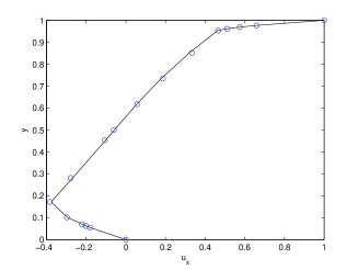
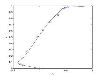
(a) $Re=1000$            (b) $Re=3200$

Figure 1: Velocity ($u_{x}$) profiles along the vertical line passing through the geometric center of the cavity. Black solid lines: (a) single-step scheme, (b) multistep scheme with index $m=2$; Blue circle lines: Ghia et al. [27]

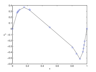
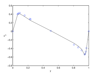
(a)$Re=1000$            (b)$Re=3200$

Figure 2: Velocity ($u_{y}$) profiles along the horizontal line passing through the geometric center of the cavity. Black solid lines: (a) single-step scheme, (b) multistep scheme with index $m=2$; Blue circle lines: Ghia et al. [27]

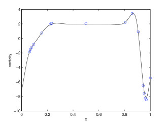
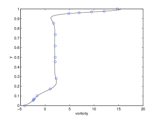
Figure 3: Vorticity values along the vertical line $x=0.5$ (left) and the horizontal line $y=0.5$ (right) passing through the geometric center of the cavity with $Re=1000$. Black solid lines: single-step scheme; Blue circle lines: Botella et al. [29]

5 Concluding remarks

We have proposed a new splitting method for solving time-dependent convection-dominated diffusion problems. A pure convection problem and a pure diffusion problem are solved successively at each iteration of the method. Explicit schemes are proposed for the time discretization of the convective problem. The explicitness of the scheme may cause a severe restriction on the time step size, which can be essentially improved by an explicit multistep scheme with smaller time step sizes so that the resulting method behaves like an unconditionally stable method. The diffusion problem involved at each iteration is always self-adjoint and coercive so that it can be solved efficiently using many existing optimal preconditioned iterative solvers. The optimal convergence orders have been confirmed by several numerical examples with smooth solutions. The schemes are then extended for the Navier-Stokes equations, where the nonlinearity is resolved by a linear explicit multistep scheme at the convection step, while only a generalized Stokes problem is needed to solve at the diffusion step and the major stiffness matrix stays invariant in the time marching process. Numerical simulations are presented to demonstrate the stability, convergence and performance of the single-step and multistep variants of the new schemes. The effectiveness and robustness of the new schemes are finally well demonstrated by the benchmark lid-driven cavity flow problem. The newly proposed schemes are all free from tuning some stabilization parameters as the most existing schemes require for the convection-dominated diffusion problems. Finally we note that the proposed fully discrete schemes are only first order in time, and we are currently investigating the potential schemes which have second order temporal accuracy.

References

- [1] A. Quarteroni and A. Valli, Numerical Approximation of Partial Differential Equations, Springer-Verlag, Berlin, 1994.
- [2] J. Donea and A. Huerta, Finite Element Methods for Flow Problems, Wiley, New York, 2003.
- [3] R. Glowinski and P. Le Tallec, Augmented Lagrangian and Operator Splitting Methods in Nonlinear Mechanics, SIAM, Philadelphia, 1989.
- [4] T.J.R. Hughes and A.N. Brooks, A multidimensional upwind scheme with no crosswind diffusion, In T.J.R. Hughes, ed., Finite Element Methods for Convection Dominated Flows, ASME, New York, 1979, 19-35.
- [5] A.N. Brooks and T.J.R. Hughes, Streamline upwind/Petrov-Galerkin formulations for convection dominated flows with particular emphasis on the incompressible Navier-Stokes equations, Comput. Methods Appl. Mech. Engrg. 32 (1982), 199-259.
- [6] T.J.R. Hughes, L. P. Franca and G.M. Hulbert, A new finite element formulation for computational fluid dynamics: VIII. The Galerkin/least-squares method for advective-diffusive equations, Comput. Methods Appl. Mech. Engrg. 73 (1989), 173-189.
- [7] M. Stynes, Steady-state convection-diffusion problems, Acta Numer. 14 (2005), 445-508.
- [8] V. John and J. Novo, Error Analysis of the SUPG Finite Element Discretization of Evolutionary Convection-Diffusion-Reaction Equations, SIAM J. Numer. Anal. 49 (2011), 1149-1176.
- [9] L.P. Franca, S.L. Frey and T.J.R. Hughes, Stabilized finite element methods: I. Application to the advective-diffusive model, Comput. Methods Appl. Mech. Engrg. 96 (1992) 253-276.
- [10] L.P. Franca and S.L. Frey, Stabilized finite element methods: II. The incompressible Navier-Stokes equations, Comput. Methods Appl. Mech. Engrg. 99 (1992), 209-233.
- [11] L.P. Franca and C. Farhatb, Bubble functions prompt unusual stabilized finite element methods, Comput. Methods Appl. Mech. Engrg. 123 (1995), 299-308.
- [12] L.P. Franca and F. Valentin, On an improved unusual stabilized finite element method for the advective-reactive-diffusive equation, Comput. Methods Appl. Mech. Engrg. 190 (2000), 1785-1800.
- [13] T.J.R. Hughes, Multiscale phenomena: Green s functions, the Dirichlet-to-Neumann formulation, subgrid-scale models, bubbles and the origin of stabilized methods, Comput. Methods Appl. Mech. Engrg. 127 (1992), 387-401.
- [14] T.J.R. Hughes, G.R. Feijo, L. Mazzei and J.-B. Quincy, The variational multiscale method a paradigm for computational mechanics, Comput. Methods Appl. Mech. Engrg. 166 (1998), 3-24.
- [15] T.J.R. Hughes, L. Mazzei and K.E. Jensen, The large eddy simulation and the variational multiscale method, Comput. Vis. Sci. 3 (2000), 47-59.
- [16] V. John, S. Kaya and W. Layton, A two-level variational multiscale method for convection-dominated convection-diffusion equations, Comput. Methods Appl. Mech. Engrg. 195 (2006), 4594-4603.
- [17] C.M. Chen and V. Thome, The lumped mass finite element method for a parabolic problem, J. Austral. Math. Soc. Ser. B 26 (1985), 329-354.
- [18] O.C. Zienkiewicz and R. Codina, Search for a general fluid mechanics algorithm, In: D.A. Caughey, M.M.Hafez, eds., Frontiers of Computational Fluid Dynamics, Wiley, New York, 1995, 101-113.
- [19] O.C. Zienkiewicz and R. Codina, A general algorithm for compressible and incompressible flow part I: The split, characteristic-based scheme, Int. J. Numer. Meth. Fluids 20 (1995), 869-885.
- [20] O.C. Zienkiewicz, P. Nithiarasu, R. Codina, M. Vzquez and P. Ortiz, The characteristic-based-split procedure: an efficient and accurate algorithm for fluid problems, Int. J. Numer. Meth. Fluids 31 (1999), 359-392.
- [21] P. Nithiarasu, O.C. Zienkiewicz and R. Codina, The Characteristic-Based Split (CBS) scheme - a unified approach to fluid dynamics, Int. J. Numer. Meth. Engrg. 66 (2006), 1514-1546.
- [22] O.C. Zienkiewicz, R.L. Taylor and P. Nithiarasu, The Finite Element Method for Fluid Dynamics (6th Edition), Elsevier, Amsterdam, 2005.
- [23] A.J. Chorin, Numerical solution of the Navier-Stokes equations, Math. Comp. 22 (1968), 745-762.
- [24] R. Temam, Sur l’approximation de la solution des equations de Navier-Stokes par la mthode des fractionnarires II, Arch. Rational Mech. Anal. 33 (1969), 377-385.
- [25] C. Taylor and P. Hood,A numerical solution of the Navier-Stokes equations using the finite element technique, Computers & Fluids 1 (1973), 73-100.
- [26] V. John, G. Matthies and J. Rang, A comparison of time-discretization/linearization approaches for the incompressible Navier-Stokes equations, Comput. Methods Appl. Mech. Engrg. 195 (2006), 5995-6010.
- [27] U. Ghia, K. N. Ghia and C. T. Shin, High-resolutions for incompressible flow using the Navier-Stokes equations and a multigrid method, J. Comput. Phys. 48 (1982) ,387-411.
- [28] E. Erturk, T.C. Corke and C. Gökçöl, Numerical solutions of 2-D steady incompressible driven cavity flow at high Reynolds numbers, Int. J. Numer. Meth. Fluids 48 (2005), 747-774.
- [29] O. Botella And R. Peyret, Benchmark spectral results on the Lid-driven cavity flow, Computers & Fluids, 27 (1998), 421-433.