Inflation in Higher Dimensional Gauss-Bonnet Cosmology

Abstract

A Gauss-Bonnet term naturally appears in the action for gravity when one considers the existence of space time with dimensions more than 1+3. A variety of inflationary models can be obtained within such a framework, once the scale factor for the hidden dimension(s) is not constrained to be the same as that of the visible ones. In particular, the need for an adhoc inflaton field is eliminated. The phase space has a rich structure with different types of solutions, both stable and unstable. For a large class of solutions, the scale factors rapidly approach an asymptotic exponential form. Furthermore, sufficient inflation can be obtained for only a modest compression of the hidden world, if the latter is of a sufficiently large dimension.

I Introduction

The prospect of gravity propagating in a space of dimensions larger than the canonical $(1+3)$ has long been an intriguing one. Apart from being a natural generalization of General Relativity, the idea has proffered tantalizing visions of both a way out of many vexing issues in high energy physics as well as that of unification of gravity with other forces. Starting with the efforts of Kaluza and KleinKK1 ; KK2 , passing through the formulation of theories in both large extra dimensions as well as small but warped extra dimensions, to gravity theories being duals to strongly coupled quantum field theories, it has been a riveting saga. Added to this has been the promise of String Theory as a path to both a consistent quantum theory of gravity as well as unification with the strong and electroweak forces.

Naturally, this has also lead to the formulation of cosmology in space-times with a larger number of dimensions, and the literature abounds with a number of such scenarios. These encompass both models wherein the visible world is confined to the usual $(1+3)$-dimensions, viz. the braneworld modelsRS1 ; RS2 ; ADD ; maeda , as well as those where we traverse the entire gamut of extra dimensions (with the latter, perforce, now being compactified with a sub-attometer radius).

Whatever be the details of such models, it is quite apparent that the presence of such extra dimensions would make themselves manifest at suitably high energies, for the extra degrees of freedom associated could then be excited. Verily, this is the guiding principle for both collider searches as well as the study of their role in quantum corrections to low-energy processes. In a similar vein, their role in the dynamics of the universe as a whole would be more pronounced when the available energy was large, or equivalently when the distance scales were small, in other words, the era of the early universe.

If we contemplate the quantum nature of gravity, it is almost self-evident that the familiar Einstein equations cannot represent the whole story. Even if one started with the Einstein-Hilbert action at the classical level, quantum corrections would generate higher derivative terms in the effective action. The form of the latter, at first glance, is protected only by the symmetries of the theory, which in the present case, is general covariance. While this requirement, by itself, is not very restrictive, one may treat the additional terms as a power series in curvature (or, rather, in scalars formed out of the curvature tensor) and, in a phenomenological treatment, confine oneselves to the lowest non-trivial terms in this expansion. Even then, three different terms are possible. One particular combination viz. the Gauss-Bonnet termLovelock ; naresh ; madore , is of particular interest both on account of certain interesting properties to be discussed below and for being the lowest order correction to the Einstein-Hilbert action as evaluated within String Theoryboulware . In terms of the Riemann tensor $R_{\mu\nu\phi\zeta}$, the Ricci tensor $R_{\mu\nu}$ and the Ricci scalar $R$, it can be expressed as

$$\textit{G}\,=\,R^{2}\,-\,4R_{\mu\nu}\,R^{\mu\nu}\,+\,R_{\mu\nu\phi\zeta}\,R^{\mu\nu\phi\zeta}\ .$$ (1)

Interestingly, in $(1+3)$-dimensions, this is but a topological term and adds little to geometrodynamics. In a space of higher dimensions, this is no longer the case and the addition of this term to the action can lead to non-trivial modifications to the equations of motion, thereby giving rise to interesting effects. In this paper, we will analyze some of the features of such a theory in context of the early universe.

In section 2, we look at the evolution equations and the conservation equation, following by section 3 which lists all the cosmological solutions and discusses the behaviour of the scale factors for both the visible and the extra dimensions. In the end, i.e., section 4, we summarize the paper and give conclusions.

II Evolution Equations

The Einstein equations, as derived for the Einstein-Hilbert action are second-order in the derivatives of the dynamical variable, viz. the metric. This is true for any dimension of spacetime. Since the dynamics of the Universe today is well explained by this theory, it is paramount that any deviation from the Einstein-Hilbert action should essentially disappear in the context of the present-day universe atleast to first order. In particular, this motivates the thought that even for higher dimensional theories, the equations of motion need to be second order. It restricts the form of the action and the simplest term that one can write beside the Einstein-Hilbert and cosmological constant term is the Gauss-Bonnet term. Such a deformation has the further advantage in the cosmological context that on account of it being a quadratic in the curvature, it could have played a significant role in the early history of the universe, while its effect today would be negligible.

We consider the higher dimensional Gauss-Bonnet actionandrew ; toporensky as

$$S\,=\,\int d^{4+D}x\sqrt{-g}\,\left[{\cal L}_{m}-\frac{M^{D+2}}{2}(\lambda R\,+\epsilon\,\textit{G})\right]$$ (2)

where $R$ and $g$ correspond to the $(1+3+D)$ dimensional curvature scalar and determinant of the metric tensor respectively. Although we have not added a cosmological constant term explicitly, we can always if intended, do so by adding an appropriate piece in the ‘matter’ lagrangian $\cal L$. $M$ defines the scale of quantum gravity in the entire bulk, and is related to $M_{\rm Planck}$ (defined in $4$-dimensions) through $V_{D}M^{D+2}\,=\,M^{2}_{\rm Planck}$, where $V_{D}$ is volume of the extra-dimensional subspace. One would expect that $V_{D}\gtrsim M^{-D}$ and, thus $M\lesssim M_{\rm Planck}$. The quantity $\epsilon$ parametrizes the weight of the Gauss-Bonnet term and can be reexpressed as $\epsilon\,=\,\gamma M^{-2}$ where $\gamma$ is a dimensionless constant. If the Gauss-Bonnet term is the result of quadratic corrections, then one would typically expect $|\gamma|<1$. The two choices $\lambda=+1(-1)$ correspond to attractive(repulsive) gravity in the Newtonian limit. While $\lambda=-1$ is not unreasonable in an epoch where the Gauss-Bonnet term dominates, clearly it is untenable at late times (i.e., the present epoch) where the curvature is small and the standard Einstein-Hilbert action needs to be recovered. We shall, then, assume $\lambda=+1$. It should be noted that String Theory predicts that $\gamma<0$, a resultboulware ; paul that we shall adopt.

What we can demand purely from observations is the homogeneity and isotropy of the normal $3-$dimensional space. If this is the only constraint to be satisfied, the line elment can be expressed as

$$ds^{2}=-dt^{2}+a^{2}(t,x^{I})\left(\frac{dr^{2}}{1-k_{1}r^{2}}+r^{2}d\Omega\right)+2g_{0I}dtdx^{I}+g_{JK}dx^{J}dx^{K}.$$ (3)

We will, however, resort to a simplification in which the hidden space is also homogeneous and isotropic. Neither the observed homogeneity and isotropy nor any other conclusion about observable cosmology that we shall draw is contingent on this assumption. On the other hand, this serves to constrain the degrees of freedom in the theory, thereby enhancing its falsifiability. The scale factor $a(t)$ will, then, be a function only of time. Similarly, the extra dimensional sector of the line element can also be expressed in a form similar to the normal dimension with its own scale factor, $b(t)$. While both these sub-spaces are isotropic among themselves, the overall space-time is manifestly anisotropic. This feature is built into the formalism by allowing $a(t)$ and $b(t)$ to be different. Such a space-time which has one temporal dimension, $3$ ‘visible’ spatial dimensions and $D$ extra spatial dimensions, can be described by the line element,

$$ds^{2}=-dt^{2}+a^{2}(t)\left(\frac{dr^{2}}{1-k_{1}r^{2}}+r^{2}d\Omega\right)+b^{2}(t)\left(\frac{dR^{2}}{1-k_{2}R^{2}}+R^{2}d\Omega_{D-1}\right).$$ (4)

We denote the time dimension with super(sub)script ‘$0$’. Whereas we reserve lower-case Roman indices ($i,j=1,2,3$) for the normal spatial dimensions, upper case Roman indices denote the extra dimensions and take values $I,J=4,5,\dots,D+3$. The observable universe is well described by a vanishing spatial flatness and hence $k_{1}=0$. For the sake of simplicity, we likewise assume the extra dimensional curvature to be vanishing, i.e. $k_{2}=0$. In other words, our spacetime manifold is described by $M^{4}\times T^{D}$.

Starting from equation (2), the Euler-Lagrange equation for the metric would read

$$\tilde{G}^{\mu}_{\nu}=\frac{1}{M^{2+D}}\,T^{\mu}_{\nu}$$ (5)

where $T^{\mu}_{\nu}$ is the $1+3+D$ dimensional stress-energy tensor for the matter content, and the generalised Einstein tensor $\tilde{G}^{\mu}_{\nu}$ incorporates the contribution from the Gauss-Bonnet term. Its non-zero components are given by

$$\tilde{G}_{0}^{0} = -\lambda\left[3\,\frac{\dot{a}^{2}}{a^{2}}+3\,D\frac{\dot{a}}{a}\frac{\dot{b}}{b}+{}^{D}\!C_{2}\frac{\dot{b}^{2}}{b^{2}}\right]+\epsilon\,\left[D\,\frac{\dot{a}^{3}\dot{b}}{a^{3}b}+36\,{}^{D}\!C_{2}\,\frac{\dot{a}^{2}\dot{b}^{2}}{a^{2}b^{2}}+18\,{}^{D}\!C_{3}\,\frac{\dot{a}\dot{b}^{3}}{ab^{3}}+12\,{}^{D}\!C_{4}\frac{\dot{b}^{4}}{b^{4}}\right]$$ (6)

$$\tilde{G}_{i}^{i} = 4\,\epsilon\,\left[2\,D\frac{\ddot{a}\dot{a}\dot{b}}{a^{2}b}+2\,{}^{D}\!C_{2}\,\frac{\dot{b}^{2}\ddot{a}}{b^{2}a}+D\,\frac{\dot{a}^{2}\ddot{b}}{a^{2}b}+3\,{}^{D}\!C_{3}\,\frac{\dot{b}^{2}\ddot{b}}{b^{3}}+3\,{}^{D}\!C_{2}\,\frac{\dot{a}^{2}\dot{b}^{2}}{a^{2}b^{2}}+6\,{}^{D}\!C_{3}\frac{\dot{b}^{3}\dot{a}}{b^{3}a}+3\,{}^{D}\!C_{4}\,\frac{\dot{b}^{4}}{b^{4}}+4\,{}^{D}\!C_{2}\frac{\ddot{b}\dot{b}\dot{a}}{b^{2}a}\right]$$ (7)

$$- \lambda\left[2\,\frac{\ddot{a}}{a}+D\,\frac{\ddot{b}}{b}+2\,D\frac{\dot{a}}{a}\frac{\dot{b}}{b}+\frac{\dot{a}^{2}}{a^{2}}+{}^{D}\!C_{2}\frac{\dot{b}^{2}}{b^{2}}\right]\qquad\forall\ i$$

$$\tilde{G}_{I}^{I} = -\lambda\,\left[(D-1)\frac{\ddot{b}}{b}+3\,\frac{\ddot{a}}{a}+3\,(D-1)\,\frac{\dot{a}}{a}\frac{\dot{b}}{b}+{}^{D-1}\!C_{2}\,\frac{\dot{b}^{2}}{b^{2}}+3\,\frac{\dot{a}^{2}}{a^{2}}\right]$$ (8)

$$+ 12\,\epsilon\left[2\,(D-1)\,\frac{\ddot{a}\dot{a}\dot{b}}{a^{2}b}+{}^{D-1}\!C_{2}\,\frac{\dot{b}^{2}\ddot{a}}{b^{2}a}+(D-1)\frac{\dot{a}^{2}\ddot{b}}{a^{2}b}+{}^{D-1}\!C_{3}\frac{\dot{b}^{2}\ddot{b}}{b^{3}}+3\,{}^{D-1}\!C_{2}\,\frac{\dot{a}^{2}\dot{b}^{2}}{a^{2}b^{2}}\right.$$

$$\left.\hskip 20.00003pt+3\,{}^{D-1}\!C_{3}\,\frac{\dot{b}^{3}\dot{a}}{b^{3}a}+{}^{D-1}\!C_{4}\,\frac{\dot{b}^{4}}{b^{4}}+2\,{}^{D-1}\!C_{2}\,\frac{\ddot{b}\dot{b}\dot{a}}{b^{2}a}+\frac{\dot{a}^{2}\ddot{a}}{a^{3}}+(D-1)\,\frac{\dot{a}^{3}\dot{b}}{a^{3}b}\right]\hskip 28.45274pt\forall\ I$$

While the Gauss-Bonnet term gives rise to terms quadrilinear in the scale factors ($a(t)$ and $b(t)$) or their derivatives, they still contain only upto the second derivatives. (This feature is not particular to the cosmological solution, but is also retained in the general case.) It is worth noting that, for $D=1$, eq.(8) is independent of $b(t)$ while this is not true for $D>1$. This distinction is of profound importance and leads to some very interesting dynamical features that some earlier effortssami , concentrated as they were on $D=1$, had missed. Indeed, the addition of the sixth, seventh and eigth dimensions, each brings into play a new term in the dynamics. Adding further to $D$ does not introduce any new term; instead, it would alter both the overall weight of the Gauss-Bonnet term relative to the Einstein-Hilbert term, and also subtly shift the balance between the various ${\cal O}(\epsilon)$ terms in the equations above, thereby affecting the dynamics.

Note that our assumption of a metric of the form of equation (4), or in other words, homogeneity and isotropy of the universe separately in the visible and the extra dimensional subspaces require that the stress-energy tensor be of the form

$$T^{\mu}_{\nu}=diag{(-\rho,P_{a},P_{a},P_{a},P_{b},....,P_{b})}$$ (9)

Here, $\rho$ is the energy density of the fluid which is present everywhere. However, the pressure it exerts on the two subspaces are different in general.

Conservation of energy-momentum $(T^{\mu}_{\nu;\mu}=0)$ implies

$$\frac{d}{dt}(\rho a^{3}b^{D})\,+\,P_{a}b^{D}\frac{da^{3}}{dt}\,+\,P_{b}a^{3}\frac{db^{D}}{dt}\,=\,0$$ (10)

For the sake of simplicity, the equations of state are assumed to yield $P_{a}=w_{a}\rho$ and $P_{b}=w_{b}\rho$, where $w_{a}$ and $w_{b}$ are constants. On solving equation (10), we, then, have

$$\rho\,=\,\rho_{0}\,\frac{a_{0}^{3(1+w_{a})}\,b_{0}^{D(1+w_{b})}}{a^{3(1+w_{a})}\,b^{D(1+w_{b})}}$$ (11)

Here, $\rho_{0}$ is the energy density corresponding to the epoch when $a=a_{0}$ and $b=b_{0}$. While we could have generalized equation (9) to include multiple fluids, this would have added little to our analysis. Hence, we desist from such complication. Indeed, as we shall see later, the matter content has relatively little importance.

III Cosmological Solutions

III.1 General features

The evolution of the Universe is governed by the Einstein’s equations (with the conservation equations being built into it.) As can be seen, we have five variables and six equations, namely the three Einstein equations (6,7,8), the conservation equation (10) and the two equations of states. However, once we Eq. 10 is considered, only one out of equations (7,8) is independent.

We start the evolution at $t=M^{-1}$. While the classical equations are involved for $t\lesssim M^{-1}$, the particular choice is just one of the convenient choices and does not have any influence on the dynamics as a result of time translation invariance. It will be convenient to express all the quantities in terms of dimensionless units, namely

$$\begin{array}[]{rcl c rcl cc}\tau&\equiv&\displaystyle t\,M&&H_{a}&\equiv&\displaystyle\frac{a^{\prime}}{a}=\frac{\dot{a}}{a\,M}\quad\quad\quad H_{b}&\equiv&\displaystyle\frac{b^{\prime}}{b}=\frac{\dot{b}}{b\,M}\\[8.61108pt] \bar{\rho}&\equiv&\displaystyle\frac{\rho}{M^{4+D}}&&\bar{P_{a}}&\equiv&\displaystyle\frac{P_{a}}{M^{4+D}}\quad\quad\quad\quad\quad\bar{P_{b}}&\equiv&\displaystyle\frac{P_{b}}{M^{4+D}}\end{array}$$ (12)

Here, prime represents derivative with repect to $\tau$. The initial value of $\tau$ is denoted by $\tau_{0}$. Note that for $k_{1,2}=0$, the equations are independent of the absolute values of $a(t)$ and $b(t)$ but depend only on the values relative to those at present time. This is reflected by the fact that $a(t)$ and $b(t)$ enter into the equations(for $k_{1,2}=0$) only as logarithmic derivatives.

We can re-express the Equations (6,7,8) in terms of dimensionless quantities as

$$-\bar{\rho} = -\lambda\,\left[3\,H_{a}^{2}+3\,D\,H_{a}\,H_{b}+{}^{D}\!C_{2}\,H_{b}^{2}\right]+12\,\gamma\,\left[D\,H_{a}^{3}\,H_{b}+3\,{}^{D}\!C_{2}\,H_{a}^{2}\,H_{b}^{2}+3\,{}^{D}\!C_{3}\,H_{a}\,H_{b}^{3}+{}^{D}\!C_{4}\,H_{b}^{4}\right]$$ (13)

$$\bar{P_{a}} = H_{a}^{\prime}\,f_{1}(H_{a},H_{b})+H_{b}^{\prime}\,f_{2}(H_{a},H_{b})+f_{3}(H_{a},H_{b})$$ (14)

$$\bar{P_{b}} = H_{b}^{\prime}\,f_{4}(H_{a},H_{b})+H_{a}^{\prime}\,f_{5}(H_{a},H_{b})+f_{6}(H_{a},H_{b})$$ (15)

where

$$\begin{array}[]{lcl}f_{1}(H_{a},H_{b})&\equiv&\displaystyle 2\,\left(-\lambda+\gamma\left[4\,D\,H_{a}\,H_{b}+4\,{}^{D}\!C_{2}\,H_{b}^{2}\right]\right)\\[6.45831pt] f_{2}(H_{a},H_{b})&\equiv&\displaystyle-D\,\lambda+4\,\gamma\,\left[D\,H_{a}^{2}+3\,{}^{D}\!C_{3}H_{b}^{2}+4\,{}^{D}\!C_{2}\,H_{a}\,H_{b}\right]\\[6.45831pt] f_{3}(H_{a},H_{b})&\equiv&\displaystyle-\lambda\,\left[3\,H_{a}^{2}+{}^{D+1}\!C_{2}H_{b}^{2}+2\,D\,H_{a}\,H_{b}\right]\\[4.30554pt] &+&\displaystyle\gamma\left[8\,D\,H_{a}^{3}\,H_{b}-2\,D\,(3-5D)\,H_{a}^{2}\,H_{b}^{2}+3\,(D-1)\,{}^{D}\!C_{3}\,H_{b}^{4}+8\,D\,{}^{D}\!C_{2}\,H_{a}\,H_{b}^{3}\right]\\[6.45831pt] f_{4}(H_{a},H_{b})&\equiv&\displaystyle-(D-1)\,\lambda+12\,\gamma\left[{}^{D-1}\!C_{3}\,H_{b}^{2}+2\,{}^{D-1}\!C_{2}\,H_{a}\,H_{b}+(D-1)\,H_{a}^{2}\right]\\[6.45831pt] f_{5}(H_{a},H_{b})&\equiv&\displaystyle-3\,\lambda+12\,\gamma\,\left[H_{a}^{2}+2\,(D-1)\,H_{a}\,H_{b}+{}^{D}\!C_{2}\,H_{b}^{2}\right]\\[6.45831pt] f_{6}(H_{a},H_{b})&\equiv&\displaystyle-\lambda\,\left[6\,H_{a}^{2}+{}^{D}\!C_{2}\,H_{b}^{2}+3\,(D-1)\,H_{a}\,H_{b}\right]\\[4.30554pt] &+&\displaystyle 12\,\gamma\,\left[H_{a}^{4}+{}^{D}\!C_{4}\,H_{b}^{4}+(D-1)\,\left\{3\,H_{a}^{3}\,H_{b}+(2D-3)\,H_{a}^{2}\,H_{b}^{2}+{}^{D-1}\!C_{2}\,H_{a}\,H_{b}^{3}\right\}\right]\end{array}$$ (16)

Note that eqn.(13) is invariant under the joint transformation $(H_{a},H_{b})\to(-H_{a},-H_{b})$. Similarly, $f_{i}(H_{a},H_{b})=f_{i}(-H_{a},-H_{b})$. This is reminiscent of the analogous property of the $(1+3)$–dimensional case. Thus, for an empty universe, both expanding ($H_{a}>0$) and contracting ($H_{a}<0$) solutions for the scale factor of the visible sector are equally possible and the growth (or otherwise) of the universe is determined by the initial conditions. We will return to this point later.

It is instructive to examine the structure of eqn.(13) alone, keeping dynamics aside for the moment. Being cubic in $H_{a}$, this leads to three solutions for a given $(\gamma,\bar{\rho},H_{b})$ combinations. In other words, there are three branches for the solution. In Fig.1, we depict these branches as plots of $H_{a}(H_{b})$ for specific values of $\gamma$ and $\bar{\rho}$. While $\bar{\rho}=0$ corresponds to an empty universe, $\bar{\rho}=1$ would indicate a cosmological constant comparable to the scale of quantum gravity, or in other words, the limit of applicability of the theory. Thus, during its evolution, the energy density of the universe must lie somewhere in between these limits. Depending on the values of $(\gamma,\bar{\rho},H_{b})$, the solutions for $H_{a}$ could either be all real, or one real and a complex-conjugate pair. Complex solutions are, of course, not admissible on physical grounds, and this is indicated in Fig.1 by the fact of there being only one solution for certain values of $H_{b}$.

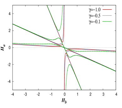
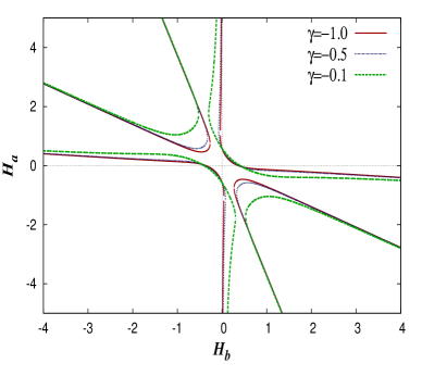
Figure 1: Curves correspond to different $\gamma$ values for $\bar{\rho}=0.0$[Left Panel] and $\bar{\rho}=1.0$[Right Panel].

Irrespective of the nature of the dynamics, it is obvious that, for a given $\bar{\rho}(t)$, the pair $(H_{b},H_{a})$ must lie on a curve that is bounded by the curves for $\bar{\rho}=0$ and $\bar{\rho}=1$. The extent to which they can move away from a specific curve is governed by the evolution of $\bar{\rho}(t)$. As Fig.1 shows, this dependence on $\bar{\rho}$ can be significant, especially for small $(H_{a},H_{b})$. However, if for some reasons, such a configuration is reached only at late times, this dependence would turn out to be irrelevant. Even a large primordial $\bar{\rho}$ would be seen to be diluted to insignificant amounts.

Before we solve for the dynamics, it is useful to dwell upon a few more issues:

• Note that we can never have both $H_{a,b}>0$ for $\bar{\rho}=0$. This is a consequence of the signs of $\gamma$ and $\lambda$, dicated as they are by other physical considerations. This, though is not true for $\bar{\rho}>0$. However, since $\bar{\rho}$ quickly decreases in magnitude to almost a vanishing value, if the visible universe is expanding at a given epoch, the hidden dimensions are contracting and vice versa.

• The above result has a striking consequence. Unless the universe started with a configuration opposite to what we have today—namely a large $b(\tau=1)$ and a small $a(\tau=1)$—we must have had a relatively small $|H_{b}(\tau)|$ during the entire history of the universe. In particular, the inflationary epoch should have had $H_{a}\gg|H_{b}|$. This immediately tells us which of the branches in Fig.1 should the initial reside on.

• It is easy to appreciate that a large value for $|H_{b}|$ in the present epoch would be inadmissible as this would lead to the effective cosmological parameters changing rapidly. Moreover, since the theory is applicable only for $b(\tau)>1$, the contraction of the hidden dimensions must have essentially stopped at some distant past. Since $H_{b}\approx 0$ implies that $H_{a}^{2}=\bar{\rho}/3\lambda$ (a result that one would have obtained in standard $(1+3)$–dimensions as well), we must have $\lambda>0$ as we have already discussed.

Since it is possible to choose initial conditions such that $|H_{b}(\tau=1)|\ll H_{a}(\tau=1)$, it is now clear (courtesy Fig.1) that this hierarchy would be maintained. This has the immediate consequence that $\bar{\rho}(\tau)$ would be a fast decreasing function of $\tau$ (see eqn.11) as long as $w_{a}>-1$ and $w_{b}$ is not very large. Since this inequality is satisfied by all ordinary matter, it is quite apparent that the universe quickly settles down to a phase where the matter density (or the pressure thereof) has little bearing on the evolution of scale factors. This result helps us understand better the assymptotic nature of the solutions to the dynamical equations that we now turn to, in particular, the lack of sensitivity to the matter content.

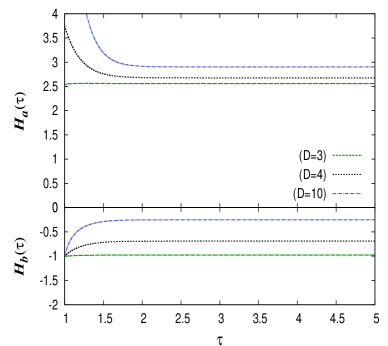
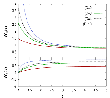
Figure 2: Behaviour of the $H_{a}$ and $H_{b}$ with the rescaled time $\tau$ for $\gamma=-0.1$ [left panel] and $\gamma=-1.0$ [right panel]. In either case, we have chosen the parameters $w_{a}=1.0/3.0$, $w_{b}=0.0$, i.e. a pure radiation confined to $(1+3)$-dimensions, and the initial conditions $\bar{\rho}(\tau=1)=1$, $H_{b}(\tau=1)=-1.0$.

For a linear equation of state (as we have assumed), we can easily eliminate $\bar{\rho}$ and $\bar{P}_{a}$ by combining eqs.(13&14). With $H_{a}=H_{a}(H_{b})$, what remains to be done is to solve a single first-order non-linear differential equation. In Fig.3, we illustrate the Hubble parameters for certain specific choices of the constants $\gamma,D$ and the initial condition $H_{b}(\tau_{0})=-1$. In each case the particular branch of the solutions $H_{a}(H_{b})$ has been chosen so as to lead to acceptable amount of inflation. Note that, in each case, $H_{b}$ initially increases from $H_{b}(\tau_{0})=-1$, only to reach a fixed point. Courtesy eqn.(13), a similar fate befalls $H_{a}$ too, with it decreasing to a positive fixed point value. Increasing $D$ has the twin effect of increasing $|H_{a}^{\rm asymp}|$ (decreasing $|H_{b}^{\rm asymp}|$), while delaying the epoch of settling at the fixed point. The dependence on $|\gamma|$ is analogous to that on $D$. This can be appreciated by realizing that the effect of the Gauss-Bonnet term becomes more pronounced with increase in $D$ and decrease in $|\gamma|$.

It is useful to consider, here, the senstivity of the evolution to the parameters $w_{a,b}$ as well as the initial condition $\bar{\rho}(\tau_{0})$. Let us consider the latter point first. As we have argued above, a comparison of the two panels of Fig.1 demonstrates that there is little difference between $\bar{\rho}=1$ and $\bar{\rho}=0$. On the other hand, naturalness demands that $\bar{\rho}\mathrel{\hbox to0.0pt{\raise 2.15277pt\hbox{$<$}\hss}{\lower 2.15277pt\hbox{$\sim$}}}1$. Thus, even though changing $\bar{\rho}(\tau_{0})$ does have a bearing on the evolution, the effect is discernible only for a small time scale (the transient region) and quickly becomes insignificant. For precisely the same reason, the effect of $w_{a,b}$ is marginal too, as long as that the energy density does not remain unchanged from a significant starting value, (i.e., unless $w_{a,b}$ conspire so that $\bar{\rho}(\tau)\sim{\cal O}(1)$ over a significant range $\tau\gg\tau_{0}$).

A constant positive $H_{a}$ (negative $H_{b}$) implies exponentially inflating visible universe (deflating hidden dimensions). In Fig.3, we illustrate the resultant scale factors. As mentioned earlier, all evolution is independent of the initial value of the scale factors. Understandably, at late times $a(\tau)$ continues to increase with the time $\tau$, while $b(\tau)$ continues to decrease. Note, though, that $a(\tau)$ cannot be inflating forever. Nor can $b(\tau)$ decrease continually, for that would either imply a current value of $b(\tau)$ to be smaller than the scale of quantum gravity (a regime beyond the validity of our treatment) or a very large initial value $b(\tau_{0})$, which, though allowed in principle, is aesthetically unpleasing. Thus the goal should be a large value of the ratio $R_{\rm end}\equiv a(\tau_{\rm end})/b(\tau_{\rm end})$, where $\tau_{\rm end}$ denotes the epoch of the end of inflation. Without going into the mechanism of ending inflation, it is clear from Fig.3 that $R_{\rm end}$ increases monotonically with $D$, and, thus, a larger $D$ proffers, in some sense, a better solution.

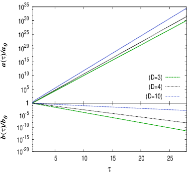
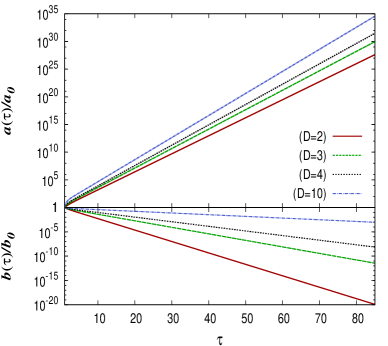
Figure 3: Behaviour of the normalized scale factors $a(\tau)$ and $b(\tau)$ with the rescaled time $\tau$ for $H_{b}(1.0)=-1.0,w_{a}=1.0/3.0$ and $w_{b}=0.0$. The left and right panels correspond to $\gamma=-0.1$ and $\gamma=-1.0$ respectively.

III.2 Asymptotic dynamics

The numerical solutions obtained in the preceding section suggest that, after a transient behaviour, the evolution, at late times asymptotes to exponential growth (decay) for the visible (hidden) sector. We examine, now, whether this feature is a generic one or is it specific to a class of initial conditions and/or parameters.

The existence of exactly exponential solutions for both $a(\tau)$ and $b(\tau)$ would, of course, be contingent on having $H_{a}^{\prime}=H_{b}^{\prime}=0$. Now, $H^{\prime}_{a,b}$ can be algebraically solved for (in terms of $H_{a,b}$) using eqns.(14&15). Vanishing derivatives of hubble parameters, thus, translate to curves in the $H_{a}$–$H_{b}$ plane (each corresponding to specific values of $\bar{P}_{a}$ and $\bar{P}_{b}$). The overlap of these curves with those corresponding to the constraint equation (13)—see, for example, Fig.1—albeit for an allowed combination $\left(\bar{\rho}(\tau),\bar{P}_{a}(\tau),\bar{P}_{b}(\tau)\right)$ would, then, indicate the fixed points. While this entails solving the full set of the dynamical equations, it is instructive to consider a special choice, namely a constant $\bar{\rho}(\tau)$. For the linear equation of state that we have assumed, this essentially implies a cosmological constant. In Fig.4, we illustrate these fixed points for a particular configuration, namely $(D=4,\ \gamma=-1.0)$.

Not all the fixed points would be stable. Stability, in this context, implies that time evolution from the neighbourhood of this point should bring $H_{a,b}$ to this point rather than take it away from it. In other words, for a small displacement from the fixed point, the derivatives $H^{\prime}_{a,b}$ should point towards the point. In Fig.4, small triangles (circles) denote the stable (unstable) fixed points. Note that each stable point $(\bar{H}_{a},\bar{H}_{b})$ is paired with an unstable one at $(-\bar{H}_{a},-\bar{H}_{b})$. This pairing can be understood by recalling that $f_{i}(H_{a},H_{b})=f_{i}(-H_{a},-H_{b})$ (see eqn.16), and, hence the derivatives must satisfy $H^{\prime}_{a,b}(\{H_{a,b}\})=-H^{\prime}_{a,b}(\{-H_{a,b}\})$. Once a stable fixed point $(H_{a}=\alpha,H_{b}=\beta)$ has been reached, the system would continue in that state, leading to exponential growth (decay) thereon.

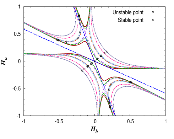
Figure 4: Phase space plot of $H_{a}$ and $H_{b}$ for $D=4$. Curves in this figure correspond to $\bar{\rho}=0.0$(solid line) and $\bar{\rho}=1.0$(dotted line) for $\gamma=-1.0$.

At this stage, it is imperative to distinguish the case of the cosmological constant from the more general scenario of an evolving $\bar{\rho}(\tau)$. Assuming a non-trivial fixed point $(\alpha,\beta)\neq(0,0)$ exists, the former must satisfy eqn.(13). On the other hand, the matter energy density (other than that for a cosmological constant) changes with time. This, immediately, demonstrates that no such fixed point can exist in the generic case. Nonetheless, as we argued earlier, for $w_{a}>-1$, the matter density quickly falls to insignificant levels (as long as we do not have $w_{b}\gg-1$), and thus, for such matter content, the asymptotic behaviour would be almost indistinguishable from that due to an empty universe.

		Stable Solutions			Unstable Solutions
$D$	$\gamma$	$\alpha$	$\beta$	$\delta=\beta/\alpha$	$\alpha$	$\beta$	$\delta=\beta/\alpha$
$2$	$-1.0$	$0.75$	$-0.54$	$-0.72$	$-0.75$	$0.54$	$-0.72$
	$-0.5$	$1.06$	$-0.77$	$-0.72$	$-1.06$	$0.77$	$-0.72$
$3$	$-1.0$	$0.81$	$-0.31$	$-0.38$	$-0.81$	$0.31$	$-0.38$
		$-0.31$	$0.81$	$-2.61$	$0.31$	$-0.81$	$-2.61$
	$-0.5$	$1.14$	$-0.44$	$-0.38$	$-1.14$	$0.44$	$-0.38$
		$-0.44$	$1.14$	$-2.59$	$0.44$	$-1.14$	$-2.59$
	$-0.1$	$2.56$	$-0.98$	$-0.38$	$-2.56$	$0.98$	$-0.38$
		$-0.98$	$2.56$	$-2.61$	$0.98$	$-2.56$	$-2.61$
$4$	$-1.0$	$0.85$	$-0.22$	$-0.26$	$-0.85$	$0.22$	$-0.26$
		$-0.39$	$0.52$	$-1.33$	$0.39$	$-0.52$	$-1.33$
	$-0.5$	$1.19$	$-0.31$	$-0.26$	$-1.19$	$0.31$	$-0.26$
		$-0.55$	$0.74$	$-1.34$	$0.55$	$-0.74$	$-1.34$
	$-0.1$	$2.67$	$-0.69$	$-0.26$	$-2.67$	$0.69$	$-0.26$
		$-1.23$	$1.66$	$-1.35$	$1.23$	$-1.66$	$-1.35$
$10$	$-1.0$	$0.92$	$-0.08$	$-0.09$	$-0.92$	$0.08$	$-0.09$
		$-0.59$	$0.22$	$-0.37$	$0.59$	$-0.22$	$-0.37$
	$-0.5$	$1.298$	$-0.11$	$-0.09$	$-1.298$	$0.11$	$-0.09$
		$-0.83$	$0.31$	$-0.37$	$0.83$	$-0.31$	$-0.37$
	$-0.1$	$2.9$	$-0.25$	$-0.09$	$-2.9$	$0.25$	$-0.09$
		$-1.85$	$0.69$	$-0.37$	$1.85$	$-0.69$	$-0.37$

Table 1: Different analytic solutions for $\rho=0$

Reverting to the cosmological constant, it is clear that, for $D=3$, the symmetry between the visible and the hidden sectors guarantees that every (un)stable fixed point $(\alpha,\beta)$ would be accompanied by another of the same ilk, namely $(\beta,\alpha)$. For $D>4$, on the other hand, no such symmetry is present, and we would, in general have two rather different stable points (each with its unstable mirror image). For $D=2$, the aforementioned three solution branches collapse to two, and the two stable fixed points merge. These features have been exhibited in Table 1.

For a given $D$, if $\gamma$ is changed, the asymptotic values $(\alpha,\beta)$ do change, but the ratio $\delta\equiv\beta/\gamma$ remains unchanged (see Table 1). This can be understood by noting that, for an empty universe, eqns.(13–15), can be trivially recast in terms of the scaled variables $\sqrt{-\gamma}\,H_{a}$ and $\sqrt{-\gamma}\,H_{b}$. The very same property dictates that the values $\alpha$ and $\beta$ are proportional to $1/\sqrt{|\gamma|}$. If we denote the epoch of reaching the fixed point by $\tau_{f}$, then, at a later time $\tau>\tau_{f}$, we have

$$\frac{a(\tau)}{b(\tau)}=\frac{a(\tau_{f})}{b(\tau_{f})}\;\exp\left[(\alpha-\beta)\,(\tau-\tau_{f})\right]$$ (17)

Thus, to maximize the growth of the ratio of the scale factors, we need to maximize the difference $(\alpha-\beta)$. Clearly, this is aided by decreasing $|\gamma|$. While this may seem paradoxical at first, this is not so given the fact that the limit $\gamma\to 0$ is not straightforward and has to be taken with care. This is demonstrated by Table 1.

The dependence of $(\alpha,\beta)$ on the number of hidden dimensions $D$ is more subtle. Analytically, it is best understood in the limit of very large $D$. Approximating, say, ${}^{D}\!C_{n}\approx D^{n}/n!$ etc., the pure-gravity version of eqns.(13–15) can now be recast in terms of $(H_{a},\widetilde{H}_{b}\equiv D\,H_{b})$ with all dependence on $D$ being absorbed in $\widetilde{H}_{b}$. This immediately implies that $\beta$ should scale as $D^{-1}$ while $\alpha$ should be free of any $D$-dependence. Of course, such a scaling is exact only in the infinite-$D$ limit, and corrections to this behaviour should be apparent for moderate $D$ values. A perusal of Table 1 show, nonetheless, that $\beta\propto D^{-1}$ is a fairly good approximation, while the relative variation in $\alpha$ is much smaller. Indeed, even these residual dependences can be understood analytically if a $1/D$ expansion is performed. For our purposes, though, such an exercise is of limited use and we shall desist from it at the current juncture. Once again, considerations analogous to those of eqn.(17) tells us that a larger $D$ value is more suitable for effecting large inflation with a moderate contraction of the hidden dimensions. Once again, Table 1 clearly demonstrates this.

III.3 End of Inflation

One issue that we have not addressed so far is the mechanism to end inflation. In different models of extra-dimensions motivated inflationary scenariosBrown ; panda ; david ; guido ; john , the issue of the end of inflation and reheating is addressed in different ways. As the scale factor of the extra-dimension decreases, it is expected that a stage is reached when quantum gravity effects become important. Our analysis, however, is of classical nature, and, hence, is not equipped to address this issue directly. Several speculations can be made though. For one, it is conceivable that quantum gravity itself would generate a pressure that would arrest such an interminable contraction, thereby forcing $a(t)$ to come out of the inflationary phase to a FRW-like one.

While this may seem to be a dissatisfactory solution, let us consider if such a situation can be reached dynamically with some (relatively) well-understood physics input. If $b(t)$ is to reach a constant value, we must impose $H_{b}=0$ and $H_{b}^{\prime}=0$ in eqns.(13,14,15). A consistent solution needs

$$\bar{\rho}\,=\,-\frac{3}{2}\,\bar{P_{a}}+\frac{\sqrt{9-96\gamma\bar{P_{b}}+72\gamma\bar{P_{a}}(2\bar{P_{a}}\gamma+3)}}{8\gamma}\ .$$ (18)

Of course, such an equation of state seems extremely unnatural and contrived. Moreover, assuming this to be an identity would not admit the dynamics that we have seen so far, and, thus, would negate the very reason for our analysis. Rather, what we need is a equation of state that, at some suitably late epoch, smoothly flows to the above or at least to a close approximation thereof. Even this flow seems a bit contrived if one considers only a single matter component. However, on the inclusion of different fields, with differing kinetic terms and potentials, such an eventuality in the evolution of the total stress-energy tensor can be managed with relative ease.

Yet another possibility arises if we treat the coefficient of the Gauss-Bonnet term ($\epsilon$) not as a constant but a dynamical quantity. This is not an unreasonable assumption for the Gauss-Bonnet term and is supposed to have arisen as the result of quantum corrections. Once $\epsilon$ is assumed to be a field, it will, naturally, evolve with time. If the potential for $\epsilon$ be such that $\epsilon=0$ is a (local) minimum, the evolution equations would naturally force the visible universe to come out of the inflating phase to a decelerating era. This issue and other associated questions such as reheating and the generation of density perturbations will be addressed in a subsequent work.

IV Conclusions and Discussions

In the context of a higher dimensional cosmology, we have, in this paper, given a mechanism to produce inflation using the Gauss-Bonnet term which provides a natural extension of the Einstein-Hilbert action. Unlike several common models of inflation where a field (called the inflaton field) is required for an inflationary phase robert ; robert1 ; shinji ; sriramkumar in the Early Universe, in our case, we have eliminated the necessity of such a field. The universe goes into an inflationary phase just from the interplay of the extra dimensions and the Gauss-Bonnet term in the action.

The parameter space characterized by the the expansion rate in the normal and extra dimensions, $H_{a}$ and $H_{b}$ , exhibits a rich structure with a variety of possible solutions depending on the initial conditions. There are both stable and unstable fixed points. If, for simplicity, linear equations of state are assumed, then the matter density dies down fast with time, as long as $w_{a}>-1$ and $w_{b}\leq 1$. Thus, asymptotically, the system reaches the limit of vacuum solution, which in our case turns out to be exponential behaviour of scale factors with time. More importantly, if one of the scale factors increase with time, the other decreases. This is a very desirable situation as we would like the normal dimensions to expand while the extra dimension should become smaller. A large expansion is achievable for a significantly wide range of the dimensionless Gauss-Bonnet parameter $\gamma$. Indeed, a $\gamma$ small enough to be consistent with a quantum-mechanical origin is admissible on this count. And while the asymptotic values of $H_{a}$ and $H_{b}$ do depend on the Gauss-Bonnet parameter, their ratio is essentially insensitive to it. For a given value of $\gamma$, the expansion rate of the visible dimensions ($H_{a}$) depends only weakly on the number of extra dimensions, $D$. On the other hand, $H_{b}$ has a stronger dependence on $D$. In fact, for large $D$, $H_{b}$ is roughly inversely proportional to $D^{-1}$.

The end of inflation, the generation of density perturbations and reheating are some of the open questions in this context. While we have proferred some possible solutions to the first of these, a detailed mechanism fulfilling all constraints needs to be worked out.

- (1) J. M. Overduin and P. S. Wesson, Kaluza-Klein gravity, Phy. Reports 283 (1997) 303
- (2) E. Witten, Search for a realistic Kaluza-Klein Theory, Nucl. Phy. B 186 (1981) 412
- (3) L. Randall and R. Sundrum, Large Mass Hierarchy from a Small Extra Dimension, Phys. Rev. Lett. 83 (1999) 3370
- (4) L. Randall and R. Sundrum, An Alternative to Compactification, Phys. Rev. Lett. 83 (1999) 23
- (5) N. Arkani-Hamed, S. Dimopoulos and G. Dvali, The hierarchy problem and new dimensions at a millimeter, Phys. Lett. B 429 (1998) 263
- (6) K. Maeda and T. Torii, Covariant gravitational equations on a brane world with a Gauss-Bonnet term, Phys. Rev. D 69 (2004) 024002
- (7) D. Lovelock, The Einstein Tensor and Its Generalizations, J. Math. Phys. 12 (1971) 498
- (8) N. Dadhich, On the Gauss-Bonnet Gravity, arXiv:hep-th/0509126v3
- (9) B. C. Paul and S. Mukherjee, Higher-dimensional cosmology with Gauss-Bonnet terms and the cosmological-constant problem, Phy. Rev. D 42 (1990) 2595
- (10) R. Chingangbam et al, A note on the viability of Gauss-Bonnet Cosmology, Phys. Lett. B, 661 (2008) 162
- (11) J. Madore, Cosmological applications of the Lanczos Lagrangian, Class. and Quan. Grav. 3 (1986) 361
- (12) D. G. Boulware and S. Deser, String-Generated Gravity Models, Phys. Rev. Lett. 55 (1985) 2656
- (13) K. Andrew, B. Bolen and C. A. Middleton, Solutions of higher dimensional Gauss-Bonnet FRW cosmology, General Relativity and Gravitation 39 (2007) 2061
- (14) D. M. Chirkov and A. V. Toporensky, On stability of power-law solution in multidimensional Gauss-Bonnet cosmology, arXiv:1212.0484
- (15) A. R. Brown, Boom and Bust Inflation: a Graceful Exit via Compact Extra Dimensions, Phys. Rev. Lett., 101 (2008) 221302
- (16) S. Panda, M. Sami and I. Thongkool, Reheating the D-brane universe via instant preheating, Phys. Rev. D, 81 (2010) 103506
- (17) D. Gherson, Constraints on the size of the extra dimension from Kaluza-Klein gravitino decay, Phys. Rev. D, 76 (2007) 043507
- (18) G. D’Amico et al, Inflation from Flux Cascades, arXiv: 1211:3416
- (19) J. H. Brodie and D. A. Easson, Brane inflation and reheating, JCAP, 12 (2003) 004
- (20) R. H. Brandenberger, Cosmology of the Early Universe, arXiv: 1003.1745
- (21) R. H. Brandenberger, A Status Review of Inflationary Cosmology, arXiv: hep-ph/0101119
- (22) S. Tsujikawa, Introductory review of cosmic inflation, arXiv: hep-ph/0304257
- (23) L. Sriramkumar, An introduction to inflation and cosmological perturbation theory, arXiv:0904.4584