Effect of Temperature Wave on Diffusive Transport of Weakly-Soluble Substances in Liquid-Saturated Porous Media

Abstract

We study the effect of surface temperature oscillations on diffusive transport of solutes of weakly-soluble substances through liquid-saturated porous media. Temperature wave induced by these oscillations and decaying deep in the porous massif creates the solubility wave along with the corresponding solute diffusion flux wave. When the non-dissolved fraction is immobilized in pores—for gases the bubbles can be immobilized by the surface tension force, for solids (e.g., limestone, gas-hydrates) the immobilization of non-dissolved phase is obvious—the only remaining mechanisms of mass transport are related to solute flux through liquid in pores. We evaluate analytically the generated time-average mass flux for the case of medium everywhere littered with non-dissolved phase and reveal the significant effect of the temperature wave on the substance release from the massif and non-dissolved mass redistribution within the massif. Analytical theory is validated with numerical calculations.

1 Introduction

Transport of gases, as well as of any weakly-soluble substances, in liquid-saturated porous media appears to possess unique features Donaldson-etal-1997 ; Donaldson-etal-1998 ; Haacke-Westbrook-Riley-2008 ; Goldobin-Brilliantov-2011 . Specifically, for a pore diameter small enough the pore-sized bubbles are immobilized by the surface tension force. The critical pore size can be readily accessed from the balance of the surface tension and buoyancy forces, which yields the value of order of $1\,\mathrm{mm}$ for the air-water system. Meanwhile, the bubbles which are large compared to the pore size will experience splitting during displacement due to the fingering instability Lyubimov-etal-2009 . As a result, the hydrodynamic transport of the gas phase through porous media becomes practically impossible for a small volumetric fraction of gas in pores (or gas saturation). The critical immobilisation gas saturation varies from system to system and depends on the time scale (e.g., the leakage process significant on the time scales of millions of years is negligible for processes evolving in days), but remains within the range from 0.5–1% Firoozabadi-Ottesen-Mikkelsen-1992 to several percent (see, e.g., Moulu-1989 ). The critical immobilized gas mass is at least one order of magnitude larger than the feasible variations of gas mass dissolved in a saturated aqueous solution of oxygen, nitrogen, or methane under the Earth’s near-surface conditions for pressure and temperature. The latter conditions are relevant for the processes in wetlands and peatbogs. Thus the principal mechanism of the gas mass transport in groundwater turns out to be the transport of gas molecules dissolved in water.

In the massif zone where the aqueous solution is saturated—i.e., porous massif is littered with bubbles of gas phase—the gas flux is solely determined by the field of solubility, which depends on pressure and temperature Pierotti-1976 ; Goldobin-Brilliantov-2011 . In this relation it is remarkable that the temperature increase from $0^{\circ}\mathrm{C}$ to $20^{\circ}\mathrm{C}$ leads to the decrease of the solubility of the main atmospheric gases and methane by a factor $1.5$. This means that the annual temperature wave propagating into the porous massif (e.g., see Yershov-1998 ) gives rise to the solubility wave of significant amplitude and associated diffusive fluxes. Hence, the annual temperature wave can significantly affect the processes of saturating groundwater with gases or methane release from wetlands and peatbogs.

The phenomenon under consideration is common and can be significant for various systems with different origins of the surface temperature oscillations, including technological systems (filters, porous bodies of nuclear and chemical reactors, etc.). However, for the sake of convenience, in this paper, we first focus on the case featured by the hydrostatic pressure gradient which is significant for geological systems, where pressure doubles on the depth of 10 meters, leading to significant change of solubility. The no pressure gradient case can be derived from the case of hydrostatic pressure by setting the gravity $g$ in resulting analytical equations to zero.

Our consideration will not be restricted to gases only. Weakly-soluble solids are very common in natural systems; these are limestone and other weakly-soluble mineral salts, methane hydrate and hydrates of other gases, etc. For these substances the immobilization of non-dissolved phase in pores is obvious. The amount of matter which can be held in the solution in pores compared to the amount of matter which can stay in the non-dissolved phase in the same pores is as small as for gases or even smaller. Solubility of these substances depends on temperature as strongly as for gases. In contrast to gases, however, the solubility of solids is not proportional to pressure but nearly independent of it. Nonetheless, the pressure inhomogeneity is owned by the hydrostatic pressure gradient, and the analytical results we will derive for gases can be downgraded to the case of solids by setting the gravity $g$ to zero, which will eliminate the pressure inhomogeneity effect on solubility, and proper correction of the temperature dependence of solubility. Thus from the view point of physics the theory for weakly-soluble solids turns out to be a specific case of the theory for gases.

We restrict our consideration to the case when the solution is saturated everywhere in the massif. This restriction is suggested not only by the motive of fundamental theoretical interest related to problem novelty but also by its practical relevance. It is relevant for the methane release from peatbogs, as the process of methane generation there can be intense enough to maintain the saturation methane-peatbogs-1 ; methane-peatbogs-2 , and for atmospheric gases. For the latter, it is important that the present time is the warm epoch against the background of the “main” cold state of 100 000-year Glacial-Interglacial cycles iceage-1 ; iceage-2 . During the cold period the groundwater is saturated with atmospheric gases under enhanced solubility conditions (low temperature), while during the warm period of diminished solubility the excessive gas mass from the solution forms gaseous bubbles in pores. For low-permeability fractureless massifs, the dominant transport mechanism is the molecular diffusion. Molecular diffusion operates with equal efficiency downwards, during the cold periods when the groundwater is being saturated with gases, and upwards, during the warm periods when the system is losing the gas mass. The longer the saturating period is, the longer duration of the release period is needed to remove the excessive amount of gases. Due to asymmetry between cold (long) and warm (short) periods groundwater in the near-surface layers should remain gas-saturated during the warm period. Thus, for the current time, one should observe gradual release of the previously saturated gases from massifs under the saturation condition. Short-time temperature waves can affect the rate of this release. Thus, we can see the relevance of the problem statement assuming the solution to be everywhere saturated.

With weakly-soluble solids, the effect can be potentially utilized in technology for filling the porous matrix with some weakly-soluble “guest” substance; the spatial mass distribution pattern of the “guest” substance can be controlled by the surface temperature waveform. For natural methane hydrate deposits in seabed sediments, the effect of temperature waves on the deposit and the gas release from it is of interest in relation to the natural Glacial-Interglacial temperature cycles and potential global climate change Hunter-etal-2013 .

In this paper, we calculate the diffusion flux of a weakly-soluble substance in the presence of temperature wave and redistribution of the mass in the non-dissolved phase. The consideration is firstly performed for gases and then downgraded to the case of solids. Both the cases of molecular diffusion and hydrodynamic dispersion are considered. The analytical results are validated with numerical simulation. The periods of negative temperatures with frozen groundwater are beyond the scope of this study and will be considered elsewhere.

2 Temperature wave in porous media with non-dissolved phase

We adopt harmonic annual oscillation of the surface temperature, $T_{0}+\Theta_{0}\cos{\omega t}$, where $T_{0}$ is the annual-mean temperature, $\Theta_{0}$ is the oscillation amplitude, and $\omega=2\pi/\mathrm{year}$. This assumption is accurate enough due to two reasons: (i) real temperature records slightly deviate from their harmonic reduction (e.g., see Yershov-1998 and fig. 1) and (ii) the penetration depth of higher harmonics into massif rapidly decreases (see eq. (1) below). With the specified surface temperature the temperature field in the half-space, which is governed by the heat diffusion equation $\partial T/\partial t=\chi\Delta T$ with no heat flux condition at infinity, is

$$T(z)=T_{0}+\Theta_{0}e^{-kz}\cos(\omega t-kz)\,,\quad k=\sqrt{\omega/2\chi}\,.$$ (1)

Here $\chi$ is the heat diffusivity, the $z$-axis is oriented downwards and its origin is on the massif surface. The pressure field is hydrostatic

$$P=P_{0}+\rho gz\,,$$ (2)

where $P_{0}$ is the atmospheric pressure, $\rho$ is the liquid (mostly, water) density, and $g$ is the gravity.

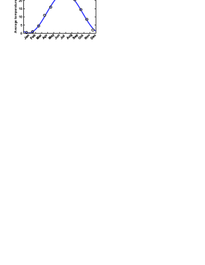
Figure 1: (Color online) Average temperature (corresponds to the surface soil temperature $T(z=0)$, eq. (1)) in New York City (circles) and its harmonic approximation (solid line) [data from open sources]

For pressure up to $10\,\mathrm{atm}$ and far from the solvent boiling temperature the solubility depends on temperature $T$ and pressure $P$ as follows Pierotti-1976

$$X^{(0)}(T,P)\simeq X^{(0)}(T_{0},P_{0})\frac{T_{0}}{T}\frac{P}{P_{0}}\exp\left[q\left(\frac{1}{T}-\frac{1}{T_{0}}\right)\right]\,,$$ (3)

where molar solubility $X^{(0)}$ is the molar amount of solute per 1 mole of solvent, $T_{0}$ and $P_{0}$ are reference values, the choice of which is guided merely by convenience reason, and $X^{(0)}(T_{0},P_{0})$ is the solubility at the reference temperature and pressure; the parameter $q\equiv-G_{i}/k_{\mathrm{B}}$, with $G_{i}$ being the interaction energy between a solute molecule and the surrounding solvent molecules, is provided in table 1. For solids the solubility approximately reads

$$X_{\mathrm{solid}}^{(0)}(T,P)\simeq X_{\mathrm{solid}}^{(0)}(T_{0},P_{0})\exp\left[q\left(\frac{1}{T}-\frac{1}{T_{0}}\right)\right]\,.$$ (4)

The instantaneous flux of molar fraction $X$ in bulk obeys

$$\vec{J}=-DX\left(\frac{\nabla X}{X}+\alpha\frac{\nabla T}{T}\right)\,,$$ (5)

where $\alpha$ is the thermodiffusion constant Bird-Stewart-Lightfoot-2007 . The importance of thermal diffusion was demonstrated for gases Goldobin-Brilliantov-2011 and methane hydrate Goldobin-CRM-2013 ; Goldobin-etal-EPJE-2014 on geological time scales.

Generally, not only solubility but all material properties of the system depend on temperature and pressure. However, feasible amplitudes of relative variations of the absolute temperature are below $5\%$. Hence, one can neglect variation of those characteristics which depend on temperature polynomially and consider variation of only those characteristics which depend on temperature exponentially: solubility (3) and the molecular diffusion coefficient $D$. Further, the only characteristic sensitive to pressure below hundreds of atmospheres is gas solubility.

Table 1: Chemical physical properties of nitrogen, oxygen, methane, and carbon dioxide (see text for details). Eq. (3) with $q$ and $X^{(0)}(T_{0},P_{0})$ specified in the table matches the experimental data from solubility-1 ; solubility-2 ; solubility-3 . Eq. (6) with $R_{d}$ and $\nu$ specified matches the experimental data from diffusion-1 ; diffusion-2 ; diffusion-3 .

	$\mathrm{N_{2}}$	$\mathrm{O_{2}}$	$\mathrm{CH_{4}}$	$\mathrm{CO_{2}}$
$q=-G_{i}/k_{\mathrm{B}}$ (K)	781	831	1138	1850
$X^{(0)}(20^{\circ}\mathrm{C},1\,\mathrm{atm})$ ($10^{-5}$)	1.20	2.41	2.60	68.7
$R_{d}$ ($10^{-10}\,\mathrm{m}$)	1.48	1.29	1.91	1.57
$\nu$ ($10^{-5}\,\mathrm{Pa\cdot s}$)	9.79	16.3	28.3	4.68

To complete the mathematical formulation of the problem, one needs to specify the dependence of molecular diffusion on temperature Bird-Stewart-Lightfoot-2007

$$D=\frac{k_{\mathrm{B}}T}{2\pi\mu R_{d}}\cdot\frac{\mu+\nu}{2\mu+3\nu}\,,$$ (6)

where $k_{\mathrm{B}}$ is the Boltzmann constant, $\mu$ is the dynamic viscosity of the solvent, $R_{d}$ is the effective radius of the solute molecules with the “coefficient of sliding friction” $\beta$, $\nu=R_{d}\beta/3$. Eq. (6) describes the bulk molecular diffusion without contributions from the effects which become important when the molecule free path is commensurable to the pore size (e.g., Berson-Choi-Pharoah-2011 ). The dependence of dynamic viscosity on temperature can be described by a modified Frenkel formula Frenkel-1955

$$\mu=\mu_{0}\exp\frac{a}{T+\tau}\,.$$ (7)

For water, coefficient $\mu_{0}=2.42\cdot 10^{-5}\,\mathrm{Pa\cdot s}$, $a=W/k_{\mathrm{B}}=570\,\mathrm{K}$ ($W$ is activation energy), and $\tau=-140\,\mathrm{K}$.

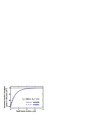
Figure 2: (Color online) Comparison of the numerically evaluated divergence of mean flux with diffusion coefficient (6) and analytical expressions (10) and (11) for annual temperature wave. Negative values of the growth rate in this figure mean dissolution of the bubbly phase.

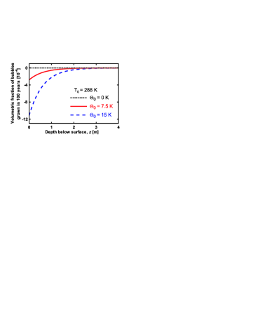
(a)	(b)
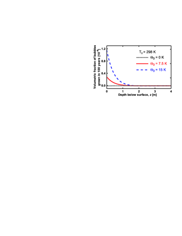
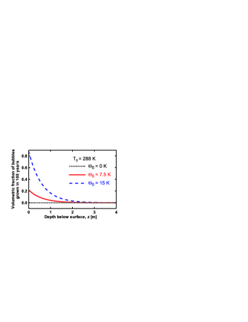
(c)	(d)

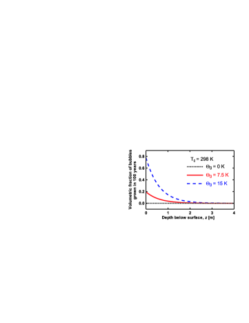
Figure 3: (Color online) The rate of bubble growth from saturated aqueous solution of methane subject to annual temperature wave. The transport mechanism is the molecular diffusion under annual-mean temperature $T_{0}=288\,\mathrm{K}$ (a) and $T_{0}=298\,\mathrm{K}$ (b), and the hydrodynamic dispersion under annual-mean temperature $T_{0}=288\,\mathrm{K}$ (c) and $T_{0}=298\,\mathrm{K}$ (d). The surface temperature oscillation amplitude $\Theta_{0}$ is specified in plots. For molecular diffusion, rough theoretical assessment $\alpha=1.8$ Goldobin-Brilliantov-2011 is adopted, although parametric study reveals the result to be nearly insensitive to the specific realistic value of $\alpha$. For hydrodynamic dispersion $D_{\mathrm{vert}}=2\cdot 10^{-7}\,\mathrm{m^{2}/s}$, which typically corresponds, e.g., to the horizontal filtration flux of groundwater $v_{\mathrm{aq}}=0.02\,\mathrm{cm/s}$ through the medium with the pore size $\sim 1\,\mathrm{mm}$ (cf. Donaldson-etal-1997 ; Donaldson-etal-1998 ).

3 Average gas mass transport

Since the diffusion transport in liquids is several orders of magnitude slower than the heat transfer, it can be well described in terms of average values over the temperature oscillation period. With the solubility law (3) diffusion flux (5) reads

$$\vec{J}=-DX^{(0)}\left[\frac{\nabla P}{P}-\left(1+\frac{q}{T}-\alpha\right)\frac{\nabla T}{T}\right]\,.$$ (8)

With expansion

$$D=D_{0}+D_{1}(T-T_{0})+\frac{1}{2}D_{2}(T-T_{0})^{2}+\dots\,,$$ (9)

where $D_{0}$, $D_{1}$, and $D_{2}$ can be plainly evaluated from eqs. (6) and (7), straightforward but laborious analytical calculations (see Appendix for details) yield mean flux

$$\left\langle J\right\rangle= -D_{0}X^{(0)}(T_{0},P_{0})\bigg{[}\frac{\rho g}{P_{0}}\left(1+A_{1}\frac{\Theta_{0}^{2}\,e^{-2kz}}{2T_{0}^{2}}\right)-\left(1+\frac{\rho gz}{P_{0}}\right)A_{2}\frac{k\Theta_{0}^{2}\,e^{-2kz}}{2T_{0}^{2}}+\mathcal{O}\left(\frac{\Theta_{0}^{4}}{T_{0}^{4}}\right)\bigg{]}\,,$$ (10)

where

$$A_{1}=1+2\frac{q}{T_{0}}+\frac{q^{2}}{2T_{0}^{2}}-\frac{D_{1}T_{0}}{D_{0}}\left(1+\frac{q}{T_{0}}\right)+\frac{D_{2}T_{0}^{2}}{2D_{0}}\,,$$

$$A_{2}=\frac{q}{T_{0}}+\left(2+\frac{q}{T_{0}}-\frac{D_{1}T_{0}}{D_{0}}\right)\left(1+\frac{q}{T_{0}}-\alpha\right).$$

We do not provide analytical expressions for $D_{1}$ and $D_{2}$ as they are extremely lengthy. These values strongly depend on temperature; nonetheless, to see the reference values of these parameters, one can evaluate from eqs. (6) and (7) for $T_{0}=300\,\mathrm{K}$ and data in table 1: $D_{1}T_{0}/D_{0}=7.39$, $7.26$, $7.12$, $7.52$ and $D_{2}T_{0}^{2}/D_{0}=28.1$, $26.6$, $25.2$, $30.2$ for $\mathrm{N_{2}}$, $\mathrm{O_{2}}$, $\mathrm{CH_{4}}$, $\mathrm{CO_{2}}$, respectively.

Beyond the penetration zone of the decaying temperature wave, i.e., for $kz\gtrsim 2$, the diffusion flux (10) is homogeneous, no gas mass accumulation or substraction is created by the flux divergence. Meantime, in the near-surface zone where the temperature wave is non-small, the flux divergence is non-zero and one observes the growth (or dissolution) of the gaseous phase;

$$\frac{\partial\left\langle X_{b}\right\rangle}{\partial t}=-\frac{\partial\left\langle{J}\right\rangle}{\partial z}\,.$$ (11)

Here $X_{b}$ is the molar amount of matter in the gaseous phase per 1 mole of all the matter in pores. The latter equation is valid for small volumetric fraction of bubbles in pores, which well corresponds to the systems we consider.

In fig. 2, one can see that analytical results involving the expansion (9) match well the results of numerical calculations, in which the expressions for the diffusion coefficient and solubility are not replaced by their truncated Taylor series, even for surface temperature oscillation amplitude $\Theta_{0}$ as large as $15\,\mathrm{K}$. Henceforth, our treatment relies entirely on these analytical results.

4 Molecular diffusion and hydrodynamic dispersion

Up to this point our results are derived for the molecular diffusion mechanism. With molecular diffusion, terms $(D_{1}T_{0}/D_{0})$ and $(D_{2}T_{0}^{2}/D_{0})$ are of the order of magnitude of $10$ ; they make principle contribution to constants $A_{1}$ and $A_{2}$, and play a decisive role in the systems evolution. Noticeably, calculations reveal the effect of thermodiffusion ($\alpha$) to be practically unobservable against the background of other contributions to the diffusion flux. Hence, the uncertainty of the value of $\alpha$ for aqueous gas solutions  is not a significant issue for the results provided in this paper.

However, along with the molecular-diffusion dominated systems, there are systems where horizontal filtration flux of groundwater is present. This flux is treated as horizontal because it is parallel to the surface and natural systems are typically much more uniform in the horizontal directions than in the vertical one. Due to the microscopic irregularity of pore geometry the filtration flux does fluid mixing which operates like an additional diffusion mechanism, the “hydrodynamic dispersion” Donaldson-etal-1997 ; Donaldson-etal-1998 ; Sahimi-1993 ; Barenblatt-Yentov-Ryzhik-2010 . Although hydrodynamic dispersion was previously studied in the relation to the evolution of atmosphere gases bubbles in aquifers Donaldson-etal-1997 ; Donaldson-etal-1998 , the effect of temperature waves was not addressed.

When hydrodynamic dispersion is present, it is typically several orders of magnitude stronger than molecular diffusion (Donaldson-etal-1997 ; Donaldson-etal-1998 ; Barenblatt-Yentov-Ryzhik-2010 , cf. in fig. 3), and the latter can be neglected. There is no analog of thermodiffusion for hydrodynamic dispersion and $\alpha=0$ for this case. Furthermore, hydrodynamic dispersion depends on the flux strength and pore geometry but not temperature, and the correlations between instantaneous flux oscillations and temperature are not obvious; therefore, $D=D_{0}$ and $D_{1}=D_{2}=0$. Finally, for hydrodynamic-dispersion dominated system, eqs. (10) and (11) yield

$$\frac{\partial\left\langle X_{b}\right\rangle}{\partial t}= D_{0}X^{(0)}(T_{0},P_{0})\left(1+\frac{2q}{T_{0}}+\frac{q^{2}}{2T_{0}^{2}}\right)\frac{\Theta_{0}^{2}}{2T_{0}^{2}}\frac{\partial^{2}}{\partial z^{2}}\left[\left(1+\frac{\rho gz}{P_{0}}\right)e^{-2kz}\right]+\mathcal{O}\left(\frac{\Theta_{0}^{4}}{T_{0}^{4}}\right).$$ (12)

In this paper we analyze both molecular-diffusion dominated systems and hydrodynamic-dispersion dominated systems.

5 Results and discussion

In fig. 3 one can see the results of calculations of the methane bubble growth rate in molecular-diffusion and hydrodynamic-dispersion dominated systems. These plots demonstrate several unique features of these cases. Let us discuss these features and their origins in detail.

Noteworthy, with molecular diffusion of methane, one can observe both bubble dissolution for lower mean temperatures (fig. 3a) and bubble growth for higher mean temperatures (fig. 3b). This is dominantly controlled by parameters $(D_{1}T_{0}/D_{0})$ and $(D_{2}T_{0}^{2}/D_{0})$ and may vary from gas to gas. Analytical expression (10) contains both exponential and linear in $z$ terms and multipliers. With purely exponential terms, the shape of the bubble growth rate profile would be determined only by $k$ [see eq. (10)]. Owing to the linear in $z$ multiplier in eq. (10), this tolerance of the profile shape to parameters $A_{1}$ and $A_{2}$ is broken by the competition between terms $e^{-2kz}$ and $ze^{-2kz}$. In particular, figs. 3a and 3b demonstrate that the penetration depth of the bubble depletion zone is nearly twice bigger than the penetration depth of the growth zone.

On the contrary, for hydrodynamic-dispersion dominated systems, only growth of bubbles is possible. According to eq. (12), the shape of the bubble growth rate profile is determined by the second $z$-derivative term. This derivative profile depends on $k=\sqrt{\omega/2\chi}$. The second $z$-derivative is everywhere positive for $k>\rho g/P_{0}=0.1\,\mathrm{m^{-1}}$, i.e., for temperature wave penetration depth below $10\,\mathrm{m}$, while for $k<\rho g/P_{0}$ it turns negative in the upper zone above $z_{*}=k^{-1}-P_{0}/\rho g$. Since for natural systems the penetration depth of the annual temperature wave never reaches $10\,\mathrm{m}$ Yershov-1998 , the latter case, with bubble depletion above $z_{*}$ and growth below $z_{*}$, is not feasible and can be relevant only for longer climate cycles.

We discussed our analytical results in relation to geological systems featured by the hydrostatic pressure gradient and annual temperature oscillations. Meanwhile, eqs. (10) and (12) hold valid for the systems where the hydrostatic pressure gradient is either absent or insignificant. The latter case may be, for example, daily temperature oscillation, the penetration depth of which is $0.1\,\mathrm{m}$ for soils—a depth on which the hydrostatic pressure increase is negligible. The case of no pressure gradient can be derived from eq. (10) by eliminating the gravity; one finds

$$\left\langle J\right\rangle=D_{0}X^{(0)}(T_{0},P_{0})\,A_{2}\frac{k\Theta_{0}^{2}\,e^{-2kz}}{2T_{0}^{2}}+\mathcal{O}\left(\frac{\Theta_{0}^{4}}{T_{0}^{4}}\right)\,.$$ (13)

Here we can see a non-trivial temperature wave effect on gas release for various technological and natural systems as well.

For solids, the results correspond to the case of no pressure gradient, eq. (13), with correction of the coefficient $A_{2}$ due to the solubility law (4), which differs from eq. (3) for gases;

$$A_{2,\mathrm{solid}}=\frac{q}{T_{0}}+\left(1+\frac{q}{T_{0}}-\frac{D_{1}T_{0}}{D_{0}}\right)\left(1+\frac{q}{T_{0}}-\alpha\right).$$ (14)

Thus, one can observe or achieve the same effect of a spatially distributed growth of the non-dissolved phase in porous matrix.

Controlling mass distribution pattern

One can control the pattern of the growth of the non-dissolved phase. Let us discuss this possibility for the case of solid substances. According to eq. (13), the surface temperature oscillation waveform

$$\Theta(z=0,t)=\int_{-\infty}^{+\infty}\theta(\omega)\,e^{i\omega t}\mathrm{d}\omega$$

produces the average growth rate

$$-\frac{\partial\langle{J}\rangle}{\partial z} =\frac{4D_{0}X^{(0)}(T_{0},P_{0})\,A_{2}}{T_{0}^{2}}\int_{0}^{+\infty}k^{2}|\theta(\omega)|^{2}\,e^{-2kz}\mathrm{d}\omega$$

$$=\frac{\chi D_{0}X^{(0)}(T_{0},P_{0})\,A_{2}}{T_{0}^{2}}\int_{0}^{+\infty}\kappa^{3}\left|\theta\left(\frac{\chi\kappa^{2}}{2}\right)\right|^{2}\,e^{-\kappa z}\mathrm{d}\kappa\,.$$ (15)

(The cross-terms of different frequencies, $\propto\theta(\omega)\theta(-\omega^{\prime})$ with $\omega\neq\omega^{\prime}$, yield vanishing time-average contributions.) The integral in the latter expression has a form of a Laplace integral, which can be used for representation of a function defined for $z\geq 0$, $f(z)=\int_{0}^{+\infty}F(\kappa)e^{-\kappa z}\mathrm{d}\kappa$ with real positive $F(\kappa)$; here $F(\kappa)$ is the inverse Laplace transform of function $f(z)$. Let us first consider the case of $A_{2}>0$. If one requires a growth pattern the inverse Laplace transform $F(\kappa)$ of which is real positive, i.e.,

$$-\frac{\partial\langle{J}\rangle}{\partial z}\propto\int_{0}^{\infty}a(\kappa)\,e^{-\kappa z}\,\mathrm{d}\kappa$$ (16)

with $a(\kappa)\geq 0$, this can be achieved by implementation of the surface temperature oscillation waveform $\Theta(0,t)=\int_{-\infty}^{+\infty}\theta(\omega)e^{i\omega t}\mathrm{d}\omega$, producing pattern (15). Comparing integrals in eqs. (15) and (16), one finds $a(\kappa)\propto\kappa^{3}\left|\theta\left(\chi\kappa^{2}/2\right)\right|^{2}$, which corresponds to

$$\theta(\omega)\propto\omega^{-3/4}\big{[}a\big{(}\sqrt{2\omega/\chi}\big{)}\big{]}^{1/2}\,.$$ (17)

For $A_{2}<0$, similar depletion pattern, with $(-\partial\langle{J}\rangle/\partial z)<0$, can be created. Thus, a certain class of patterns can be produced by means of a proper temperature oscillation waveform. Presumably, this can be generalized to a spatially non-unform surface temperature oscillations, allowing producing a class of three-dimensional patterns of the “guest” substance in porous matrix.

6 Conclusion

We have addressed the problem of influence of the surface temperature oscillation (and consequent temperature wave) on the gas transport through liquid-saturated porous media. Specifically, we have considered the problem for the case of saturated gas solution, i.e., when bubbles are spread everywhere in the medium. Strong exponential dependence of the solubility and the molecular diffusion coefficient on temperature has been found to lead to non-negligible instantaneous diffusion fluxes although the amplitude of the relative variation of absolute temperature does not exceed $5\%$. Due to nonlinearity these fluxes are not averaged-out to zero but create the mean mass flux.

Our main findings are expressed by eq. (10) and its reductions for hydrodynamic-dispersion dominated systems [eq. (12)] and no pressure gradient systems [eq. (13)]. These analytical equations have been shown to fairly match the results of numerical calculations (see fig. 2). We have revealed that the temperature wave can either enhance or deplete the near-surface bubbly zone in molecular-diffusion dominated systems and only enhance this zone for hydrodynamic-dispersion dominated systems (for instance, see fig. 3).

The phenomenon we have addressed is expected to be of significance not only for gases but also for any weakly-soluble substance, given its solubility is sensitive to temperature. Moreover, one can control the pattern of the growth of the non-dissolved phase.

Appendix: Calculation of average diffusion flux

Here we derive eq. (10) for the average diffusion flux from eq. (8) using expression for the solubility (3) and diffusion coefficient (9);

$$\langle J\rangle = -\bigg{\langle}\left(D_{0}+D_{1}(T-T_{0})+\frac{1}{2}D_{2}(T-T_{0})^{2}+\dots\right)$$ (18)

$$\qquad\times X^{(0)}(T_{0},P_{0})\frac{T_{0}}{T}\frac{P}{P_{0}}\exp\left[q\left(\frac{1}{T}-\frac{1}{T_{0}}\right)\right]\left[\frac{\nabla P}{P}-\left(1+\frac{q}{T}-\alpha\right)\frac{\nabla T}{T}\right]\bigg{\rangle}\,.$$

With short-hand notation $T=T_{0}(1+\vartheta)$, making expansions in $\vartheta$, one finds

$$\frac{\langle J\rangle}{D_{0}X^{(0)}(T_{0},P_{0})} = -\bigg{\langle}\left(1+\frac{D_{1}T_{0}}{D_{0}}\vartheta+\frac{D_{2}T_{0}^{2}}{2D_{0}}\vartheta^{2}\right)\left(1-\frac{q}{T_{0}}\vartheta+\left(\frac{q}{T_{0}}+\frac{q^{2}}{2T_{0}^{2}}\right)\vartheta^{2}\right)$$ (19)

$$\qquad\times\bigg{(}\frac{\rho g}{P_{0}}(1-\vartheta+\vartheta^{2})-\frac{P}{P_{0}}\left[(1-\alpha)(1-2\vartheta)+\frac{q}{T_{0}}(1-3\vartheta)\right]\nabla\vartheta\bigg{)}+\mathcal{O}(\vartheta^{3})\bigg{\rangle}\,.$$

As $\langle\vartheta\rangle=0$, $\langle\vartheta^{2}\rangle=\frac{\Theta_{0}^{2}}{2T_{0}^{2}}e^{-2kz}\neq 0$, $\langle\vartheta\nabla\vartheta\rangle=-\frac{k\Theta_{0}^{2}}{2T_{0}^{2}}e^{-2kz}\neq 0$, and $\langle\vartheta^{3}\rangle=0$, eq. (19) yields

$$\frac{\langle J\rangle}{D_{0}X^{(0)}(T_{0},P_{0})} = -\frac{\rho g}{P_{0}}-\frac{\rho g}{P_{0}}\langle\vartheta^{2}\rangle\left(1+2\frac{q}{T_{0}}+\frac{q^{2}}{2T_{0}^{2}}-\frac{D_{1}T_{0}}{D_{0}}-\frac{D_{1}q}{D_{0}}+\frac{D_{2}T_{0}^{2}}{2D_{0}}\right)$$

$$\qquad{}-\frac{P}{P_{0}}\langle\vartheta\nabla\vartheta\rangle\bigg{[}2-2\alpha+3\frac{q}{T_{0}}+\left(\frac{q}{T_{0}}-\frac{D_{1}T_{0}}{D_{0}}\right)\left(1-\alpha+\frac{q}{T_{0}}\right)\bigg{]}+\mathcal{O}(\langle\vartheta^{4}\rangle)$$

$$= -\frac{\rho g}{P_{0}}\big{(}1+A_{1}\langle\vartheta^{2}\rangle\big{)}-\frac{P}{P_{0}}A_{2}\langle\vartheta\nabla\vartheta\rangle+\mathcal{O}(\langle\vartheta^{4}\rangle)\,.$$

with $A_{1}$ and $A_{2}$ specified below eq. (10).

For solids, with solubility (4), one similarly finds

$$\frac{\langle J\rangle}{D_{0}X^{(0)}(T_{0},P_{0})} = -\frac{P}{P_{0}}\langle\vartheta\nabla\vartheta\rangle\bigg{[}1-\alpha+2\frac{q}{T_{0}}+\left(\frac{q}{T_{0}}-\frac{D_{1}T_{0}}{D_{0}}\right)\left(1-\alpha+\frac{q}{T_{0}}\right)\bigg{]}+\mathcal{O}(\langle\vartheta^{4}\rangle)$$

$$= -A_{2,\mathrm{solid}}\langle\vartheta\nabla\vartheta\rangle+\mathcal{O}(\langle\vartheta^{4}\rangle)\,.$$

with $A_{2,\mathrm{solid}}$ specified by eq. (14).

References

- (1) J.H. Donaldson, J.D. Istok, M.D. Humphrey, K.T. O’Reilly, C.A. Hawelka, D.H. Mohr, Development and Testing of a Kinetic Model for Oxygen Transport in Porous Media in the Presence of Trapped Gas, Ground Water 35, 270 (1997).
- (2) J.H. Donaldson, J.D. Istok, K.T. O’Reilly, Dissolved Gas Transport in the Presence of a Trapped Gas Phase: Experimental Evaluation of a Two-Dimensional Kinetic Model, Ground Water 36, 133 (1998).
- (3) R.R. Haacke, G.K. Westbrook, M.S. Riley, Controls on the formation and stability of gas hydrate-related bottom-simulating reflectors (BSRs): A case study from the west Svalbard continental slope, J. Geophys. Res., 113, B05104 (2008).
- (4) D.S. Goldobin, N.V. Brilliantov, Diffusive Counter Dispersion of Mass in Bubbly Media, Phys. Rev. E 84(5), 056328 (2011).
- (5) D.V. Lyubimov, S. Shklyaev, T.P. Lyubimova, O. Zikanov, Instability of a drop moving in a Brinkman porous medium, Phys. Fluids 21, 014105 (2009).
- (6) A. Firoozabadi, B. Ottesen, M. Mikkelsen, Measurements of supersaturation and critical gas saturation, SPE Formation Evaluation 7(4), 337 (1992).
- (7) J.C. Moulu, Solution-gas drive: Experiments and simulation, J. Petrol. Sci. Eng. 2, 379 (1989).
- (8) R.A. Pierotti, A scaled particle theory of aqueous and nonaqueous solutions, Chem. Rev. 76(6), 717 (1976).
- (9) E.D. Yershov, General Geocryology (Cambridge University Press, New York, 1998).
- (10) K.J. van Groenigen, C.W. Osenberg, B.A. Hungate, Increased soil emissions of potent greenhouse gases under increased atmospheric CO2, Nature 475, 214 (2011).
- (11) I. Aselmann, P.J. Crutzen, Global distribution of natural fresh-water wetlands and rice paddies, their net primary productivity, seasonality and possible methane emissions, J. Atmospheric Chem. 8(4), 307 (1989).
- (12) J.R. Petit, J. Jouzel, D. Raynaud, N.I. Barkov, et al., Climate and atmospheric history of the past 420000 years from the Vostok ice core, Antarctica, Nature 399, 429 (1999).
- (13) EPICA community members, Eight glacial cycles from an Antarctic ice core, Nature 429, 623 (2004).
- (14) S.J. Hunter, D.S. Goldobin, A.M. Haywood, A. Ridgwell, J.G. Rees, Sensitivity of the global submarine hydrate inventory to scenarios of future climate change, Earth Planet. Sci. Lett. 367, 105-–115 (2013).
- (15) R.B. Bird, W.E. Stewart, E.N. Lightfoot, Transport Phenomena (Wiley, New York, 2007).
- (16) D.S. Goldobin, Non-Fickian diffusion affects the relation between the salinity and hydrate capacity profiles in marine sediments, Comptes Rendus Mecanique 341, 386–392 (2013).
- (17) D.S. Goldobin, N.V. Brilliantov, J. Levesley, M.A. Lovell, C.A. Rochelle, P.D. Jackson, A.M. Haywood, S.J. Hunter, J.G. Rees, Non-Fickian Diffusion and the Accumulation of Methane Bubbles in Deep-Water Sediments, Eur. Phys. J. E 37, 45 (2014).
- (18) A. Berson, H.-W. Choi, J.G. Pharoah, Determination of the effective gas diffusivity of a porous composite medium from the three-dimensional reconstruction of its microstructure, Phys. Rev. E 83, 026310 (2011).
- (19) J.I. Frekel, Kinetic theory of liquids (Dover Publications, New York, 1955).
- (20) V.I. Baranenko, V.S. Sysoev, L.N. Fal’kovskii, V.S. Kirov, A.I. Piontkovskii, A.N. Musienko, The solubility of nitrogen in water, Atomic Energy 68, 162 (1990).
- (21) V.I. Baranenko, L.N. Fal’kovskii, V.S. Kirov, L.N. Kurnyk, A.N. Musienko, A.I. Piontkovskii, Solubility of oxygen and carbon dioxide in water, Atomic Energy 68, 342 (1990).
- (22) S. Yamamoto, J.B. Alcauskas, T.E. Crozier, Solubility of Methane in Distilled Water and Seawater, J. Chem. Eng. Data 21, 78 (1976).
- (23) P.T.H.M. Verhallen, L.J.P. Oomen, A.J.J.M.v.d. Elsen, A.J. Kruger, J.M.H. Fortuin, The diffusion coefficients of helium, hydrogen, oxygen and nitrogen in water determined from the permeability of a stagnant liquid layer in the quasi-steady state, Chem. Eng. Sci. 39(11), 1535 (1984).
- (24) W. Sachs, The diffusional transport of methane in liquid water: method and result of experimental investigation at elevated pressure, J. Petrol. Sci. Eng. 21, 153 (1998).
- (25) R.E. Zeebe, On the molecular diffusion coefficients of dissloved CO2, HCO, and CO and their dependence on isotopic mass, Geochimica et Cosmochimica Acta 75, 2483 (2011).
- (26) M. Sahimi, Flow phenomena in rocks: from continuum models to fractals, percolation, cellular automata, and simulated annealing, Rev. Mod. Phys. 65, 1393 (1993).
- (27) G.I. Barenblatt, V.M. Yentov, V.M. Ryzhik, Theory of Fluid Flows Through Natural Rocks (Springer, 2010).