Efficient, Broadband and Robust Frequency Conversion by Fully Nonlinear Adiabatic Three Wave Mixing

Abstract

A comprehensive physical model of adiabatic three wave mixing is developed for the fully nonlinear regime, i.e. without making the undepleted pump approximation. The conditions for adiabatic evolution are rigorously derived, together with an estimate of the bandwidth of the process. Furthermore, these processes are shown to be robust and efficient. Finally, numerical simulations demonstrate adiabatic frequency conversion in a wide variety of physically attainable configurations.

I Introduction

Frequency conversion, via three wave mixing (TWM) processes in quadratic nonlinear optical media, is widely used in order to generate laser frequencies that are not available by direct laser action Boyd_NLO_book . The efficiency of a TWM process depends on the fulfillment of a phase-matching condition Boyd_NLO_book ; Armstrong_PR_127 . Quasi-phase-matching (QPM) Boyd_NLO_book ; Armstrong_PR_127 ; Hum_CRP_8 , a method in which the sign of the nonlinear coefficient is modulated, facilitates control over phase-matching conditions. Still, QPM processes are generally not robust against variation in system parameters, such as temperature, input wavelength, incidence angle, etc.

Recently, several works have been published that concern robust adiabatic TWM processes in the fixed (undepleted) pump approximation Suchowski_PRA_78 ; Suchowski_OE_17 ; Suchowski_APB_105 ; Moses_OL_37 ; Porat_OL_35_1590 ; Porat_OE_20 ; Porat_JOSAB_29 ; Porat_APL ; Rangelov_PRA_85 , i.e. when one of the waves is much more intense than the others, and thus is negligibly affected by the interaction. This assumption linearizes the dynamics, making it isomorphous to the linear Schr dinger equation of quantum mechanics, and thus allows the use of quantum mechanical adiabatic theorem Messiah_book .

The first step towards fully nonlinear TWM was taken by Baranova et al. Baranova_QE_25 , for the special case of second harmonic generation (SHG). Phillips et al. extended the work into the realm of optical parametric amplification (OPA) and optical parametric oscillation (OPO) Phillips_OL_35 ; Phillips_OE_20 . However, these works do not provide a rigorous physical model explaining the observed phenomena. Rather, it was stated that this is a generalization of the case with fixed pump, analogous with a quantum model of a two-level atom Crisp_PRA_8 . This generalization is not self-evident, as the removal of the fixed pump approximation invalidates the analogy made with other systems. Specifically, a reference was made to the geometrical representation of TWM made by Luther et al. Luther_JOSAB_17 as being analogous to that made by Crisp Crisp_PRA_8 with regards to a nonlinear two-level atom, which builds on the Feynman, Vernon and Hellwarth model Feynman_JAP_28 . We maintain that this analogy does not hold, since the nonlinearities in the two physical systems, TWM and two-level atom, are of different nature. The dynamics of the two-level atom remains linear at all times, as the effective wave vector is governed entirely by the electric field, which is taken to be independent of the atomic state in the approximation made by Crisp. The nonlinearity is expressed in the resulting susceptibility of the atom. Contrarily, in the TWM geometrical representation, the analogous quantity to the effective wave vector is a function of the interacting field amplitudes, which renders the dynamics itself nonlinear. Two exceptions are special cases for which a sound physical model was found: (i) the case studied by Longhi Longhi_OL_32 , in which SHG was followed by sum frequency generation (SFG) to generate the third harmonic, which was found to be analogous to a certain nonlinear quantum system Pu_PRL_98 (ii) the case of OPA with high initial pump-to-signal ratio, which Yaakobi et al. Yaakobi_OE_21 approached as a case of auto-resonance.

Other groups have taken up quantum systems with fully nonlinear dynamics, and developed a theory of adiabatic evolution for them Liu_PRL_78 ; Meng_PRA_78 ; Zhou_PRA_81 . Interestingly, they base their method on representing the Schr dinger equation in a canonical Hamiltonian structure, as was done in classical mechanics, and use classical adiabatic invariance theorem Arnold_book . The equations governing TWM have also been put in a canonical Hamiltonian structure in several works Luther_JOSAB_17 ; McKinstrie_JOSAB_10 ; Trillo_OL_17 , but not in the context of adiabatic evolution.

Here, a comprehensive physical model of fully nonlinear adiabatic TWM is presented for the first time to the best of our knowledge. This analysis leads to a condition for efficient, broadband and robust frequency conversion. Such conversion is demonstrated numerically.

This paper is organized as follows. In Section II the theoretical model of TWM is presented, along with this system’s stationary states, using canonical Hamiltonian structures. In section III adiabatic evolution is analyzed, and an analysis of robustness leading to large bandwidth is provided. Section IV presents numerical simulations of adiabatic TWM with physically realistic parameters, available with current technology.

II Theoretical Model

II.1 Coupled Wave Equations in Canonical Hamiltonian Structure

The dynamics of TWM is commonly described by three coupled wave equations. Assuming plane-waves and a slowly varying envelope, the three equations are Boyd_NLO_book ; Armstrong_PR_127

$$\frac{dA_{1}}{dz} = -i\gamma_{1}A_{2}^{*}A_{3}exp\left(-i\int_{0}^{z}\Delta k\left(z^{\prime}\right)dz^{\prime}\right)$$

$$\frac{dA_{2}}{dz} = -i\gamma_{2}A_{1}^{*}A_{3}exp\left(-i\int_{0}^{z}\Delta k\left(z^{\prime}\right)dz^{\prime}\right)$$

$$\frac{dA_{3}}{dz} = -i\gamma_{3}A_{1}A_{2}exp\left(i\int_{0}^{z}\Delta k\left(z^{\prime}\right)dz^{\prime}\right)$$ (1)

where $\gamma_{j}=\chi^{\left(2\right)}\omega_{j}^{2}/\left(k_{j}c^{2}\right)$ are the coupling coefficients, and $k_{j}$ and $A_{j}$ are the wavenumber and complex amplitude of the wave at frequency $\omega_{j}$, respectively. $\chi^{\left(2\right)}$ is the second order nonlinear susceptibility and $\Delta k=k_{1}+k_{2}-k_{3}$ is the phase-mismatch. Without loss of generality we assume $\omega_{1}\leq\omega_{2}<\omega_{3}$ where $\omega_{3}=\omega_{1}+\omega_{2}$.

From this point, we follow the analysis of Luther et al. Luther_JOSAB_17 in the construction of a canonical Hamiltonian form of the coupled wave equations. First, we define $A_{j}=\sqrt{\gamma_{j}}q_{j}exp\left(-i\int_{0}^{z}\Delta k\left(z^{\prime}\right)dz^{\prime}\right)$ and note that this renders $\left|q_{j}\right|^{2}$ proportional to the photon flux at $\omega_{j}$. Next, we write the three equations using $q_{j}$,

$$\frac{dq_{1}}{d\xi} = i\Delta\Gamma q_{1}-iq_{2}^{*}q_{3}$$

$$\frac{dq_{2}}{d\xi} = i\Delta\Gamma q_{2}-iq_{1}^{*}q_{3}$$

$$\frac{dq_{3}}{d\xi} = i\Delta\Gamma q_{3}-iq_{1}q_{2}$$ (2)

where we also defined the scaled propagation length $\xi=z\sqrt{\gamma_{1}\gamma_{2}\gamma_{3}}$ and the parameter $\Delta\Gamma=\Delta k/\sqrt{\gamma_{1}\gamma_{2}\gamma_{3}}$, which describes the relative strength of the phase-mismatch compared to the nonlinearity. The coupled equations can now be written in a canonical Hamiltonian structure,

$$\frac{dq_{j}}{d\xi}=-2i\frac{\partial H}{\partial q_{j}^{*}}$$ (3)

where $q_{j}$ play the role of the generalized coordinates, $q_{j}^{*}$ are their conjugate generalized momenta and

$$H=\frac{1}{2}\left(q_{1}^{*}q_{2}^{*}q_{3}+q_{1}q_{2}q_{3}^{*}\right)-\frac{\Delta\Gamma}{2}{\displaystyle\sum_{j=1}^{3}}\left|q_{j}\right|^{2}$$ (4)

is the Hamiltonian. Additionally, we have the Poisson brackets relations

$$\left\{q_{i},q_{j}\right\} = 0\,,\,\left\{q_{i}^{*},q_{j}^{*}\right\}=0\,,\,\left\{q_{i},q_{j}^{*}\right\}=-2i\delta_{ij}$$ (5)

Finally, we note that the Hamiltonian is invariant under the phase transformations

$$\left(q_{1},q_{2},q_{3}\right) \rightarrow \left(q_{1}exp\left(i\theta_{1}\right),q_{2},q_{3}exp\left(i\theta_{1}\right)\right)$$ (6)

$$\left(q_{1},q_{2},q_{3}\right) \rightarrow \left(q_{1}exp\left(i\theta_{2}\right),q_{2}exp\left(-i\theta_{2}\right),q_{3}\right)$$ (7)

$$\left(q_{1},q_{2},q_{3}\right) \rightarrow \left(q_{1},q_{2}exp\left(i\theta_{3}\right),q_{3}exp\left(i\theta_{3}\right)\right)$$ (8)

which can readily be shown to be generated by the Manley-Rowe relations,

$$K_{1} = \left|q_{1}\right|^{2}+\left|q_{3}\right|^{2}$$

$$K_{2} = \left|q_{1}\right|^{2}-\left|q_{2}\right|^{2}$$

$$K_{3} = \left|q_{2}\right|^{2}+\left|q_{3}\right|^{2}$$ (9)

i.e. the $K_{j}$ are constants of the motion.

II.2 Stationary States

The stationary states are very significant for the adiabatic evolution analyzed in section III. It will be shown there that when an adiabaticity condition is satisfied, the system evolves along these states as they follow a slowly changing system parameter - the phase-mismatch. Determining the dependence of these states on phase-mismatch is thus crucial for predicting the outcome of adiabatic evolution.

The TWM system is known to have two stationary states Kaplan_OL_18 besides the trivial ones, i.e. the states where two of the three waves have no energy. For completeness, they will be derived here as well. We note that any parametric instabilities are ignored here, as we seek only stable solutions.

In a stationary state, the state of the system is transformed into itself by the evolution dynamics. The coupled wave equations 2 are invariant with respect to the transformation

$$\left(q_{1},q_{2},q_{3}\right)\rightarrow\left(q_{1}exp\left(i\theta_{1}\xi\right),q_{2}exp\left(i\theta_{2}\xi\right),q_{3}exp\left[i\left(\theta_{1}+\theta_{2}\right)\xi\right]\right)$$ (10)

as evident from Eq. 6 and 8. If

$$\frac{dq_{j}}{d\xi} = i\theta_{j}q_{j}\,,\,j=1,2$$

$$\frac{dq_{3}}{d\xi} = i\left(\theta_{1}+\theta_{2}\right)q_{3}$$ (11)

then Eq. 2 will perform the transformation 10 and remain invariant, i.e. the system state will be transformed into itself. Therefore, Eq. 11 define the stationary states for this system. Substituting these relations in Eq. 2 yields quartic equations of $\theta_{1}$ and $\theta_{2}$, with the Manley-Rowe relations as parameters. For any given pair of Manley-Rowe constants, there exist $\theta_{1}$ and $\theta_{2}$ that yield two nontrivial stationary states, which we hence term the “plus state” and “minus state”, and use corresponding indexes in mathematical expressions. These solutions are very involved algebraically, and do not facilitate physical insight. We therefore focus first on the special case where the two low frequencies have the same photon flux, i.e. $\left|q_{1}\right|^{2}=\left|q_{2}\right|^{2}$ (note that still, generally, $\omega_{1}\neq\omega_{2}$), which leads to two simple solutions:

$$q_{1}^{+}=q_{2}^{+} =$$

$$\begin{cases}\sqrt{\left(\Delta\Gamma-\theta_{+}\right)\left(\Delta\Gamma-2\theta_{+}\right)}exp\left(i\theta_{+}\xi\right)&,\Delta\Gamma>-\sqrt{2P_{3}}\\ 0&,\Delta\Gamma<-\sqrt{2P_{3}}\end{cases}$$

$$q_{3}^{+} =\begin{cases}\left(\Delta\Gamma-\theta_{+}\right)exp\left(2i\theta_{+}\xi\right)&,\Delta\Gamma>-\sqrt{2P_{3}}\\ -\sqrt{\frac{P_{3}}{2}}\cdot exp\left(i\Delta\Gamma\xi\right)&,\Delta\Gamma<-\sqrt{2P_{3}}\end{cases}$$ (12)

and

$$q_{1}^{-}=q_{2}^{-} =$$

$$\begin{cases}\sqrt{\left(\Delta\Gamma-\theta_{-}\right)\left(\Delta\Gamma-2\theta_{-}\right)}exp\left(i\theta_{-}\xi\right)&,\Delta\Gamma<\sqrt{2P_{3}}\\ 0&,\Delta\Gamma>\sqrt{2P_{3}}\end{cases}$$

$$q_{3}^{-} =\begin{cases}\left(\Delta\Gamma-\theta_{-}\right)exp\left(2i\theta_{-}\xi\right)&,\Delta\Gamma<\sqrt{2P_{3}}\\ \sqrt{\frac{P_{3}}{2}}\cdot exp\left(i\Delta\Gamma\xi\right)&,\Delta\Gamma>\sqrt{2P_{3}}\end{cases}$$ (13)

where

$$\theta_{\pm} = \frac{5\Delta\Gamma\pm\sqrt{\Delta\Gamma^{2}+6s^{2}P_{3}}}{6}$$

$$P_{3} \equiv K_{1}+K_{3}$$ (14)

The normalized photon flux of each of the three waves, as a function of the normalized (dimensionless) phase-mismatch $\Delta\Gamma/\sqrt{P_{3}}$, for each of the stationary states, is plotted in Fig. 1, for the case where $\left|q_{1}\right|^{2}=\left|q_{2}\right|^{2}$. For the minus state, as $\Delta\Gamma/\sqrt{P_{3}}$ approaches $-\infty,$ the photon flux of the waves with the two lower frequencies (i.e. $\omega_{1}$ and $\omega_{2}$) approaches $P_{3}/2$. It monotonically decreases with increasing $\Delta\Gamma/\sqrt{P_{3}}$ up to $\Delta\Gamma/\sqrt{P_{3}}=\sqrt{2}$, where it vanishes and stays nulled for any $\Delta\Gamma/\sqrt{P_{3}}>\sqrt{2}$. The high frequency wave ($\omega_{3}$) photon flux approaches $0$ for $\Delta\Gamma/\sqrt{P_{3}}\rightarrow-\infty$, monotonically increases with $\Delta\Gamma/\sqrt{P_{3}}$ up to $\Delta\Gamma/\sqrt{P_{3}}=\sqrt{2}$, and stays constant at $P_{3}/2$ for any $\Delta\Gamma/P_{3}>\sqrt{2}$. The dependence of the plus state intensities on $\Delta\Gamma$ is the mirror image, around $\Delta\Gamma=0$, of the minus state’s intensities dependence, i.e. $\left|q_{j}^{+}\left(\Delta\Gamma\right)\right|^{2}=\left|q_{j}^{-}\left(-\Delta\Gamma\right)\right|^{2}$. Note that where $\left|q_{1}^{\pm}\right|^{2}=\left|q_{2}^{\pm}\right|^{2}=0$ the stationary states are in fact trivial.

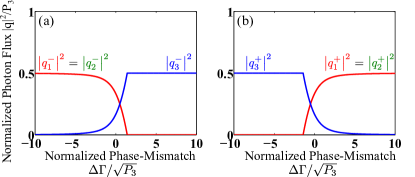
Figure 1: Normalized photon flux of each wave of the two stationary states with $\left|q_{1}\right|^{2}=\left|q_{2}\right|^{2}$. (a) Minus state. (b) Plus state.

Fig. 2 shows the photon flux of each wave of the stationary states with the same parameters, for the case where $\left|q_{1}\right|^{2}\neq\left|q_{2}\right|^{2}$. For the minus state, the three waves have the same monotonic dependence on $\Delta\Gamma/\sqrt{P_{3}}$ as in the special case of $\left|q_{1}\right|^{2}=\left|q_{2}\right|^{2}$, except that the two low frequency waves do not vanish (the kink that was observed at $\Delta\Gamma/\sqrt{P_{3}}=\sqrt{2}$ in Fig. 1 is now missing). Instead, of these two waves, the one that has the lower photon flux ($\left|q_{2}^{-}\right|^{2}$ in Fig. 2a) asymptotically approaches zero, while the other one remains at a constant difference from it, which corresponds to the value of $K_{2}$ that characterizes this state. Since the stationary state is also characterized by a certain value of $K_{3}$, $\left|q_{3}^{-}\right|^{2}$ always complements $\left|q_{2}^{-}\right|^{2}$ to maintain the same $K_{3}$. These stationary states are thus never trivial. Furthermore, as before, $\left|q_{j}^{+}\left(\Delta\Gamma\right)\right|^{2}=\left|q_{j}^{-}\left(-\Delta\Gamma\right)\right|^{2}$.

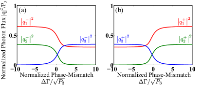
Figure 2: Normalized photon flux of each wave of the two stationary states with $K_{2}/\left(K_{1}+K_{3}\right)=0.3$. (a) Minus state. (b) Plus state.

II.3 Dimensionally Reduced Canonical Hamiltonian Structure

The two previous subsections summarized representations and properties of the TWM system that were already known. In this subsection, a new representation is developed. This representation will be used in section III to account for adiabatic evolution.

The existence of the constants of the motion $K_{j}$, in addition to $H$, indicates that the number of degrees of freedom of the system is lower than the dimensionality of the $\left(q_{j},q_{j}^{*}\right)$ phase-space. As Liu et al. Liu_PRL_78 have done for systems with $U\left(1\right)$ symmetry, we’ll use these constants to produce a phase space with reduced dimensionality. We define the real generalized coordinates $Q_{j}$ and real generalized momenta $P_{j}$:

$$Q_{1} = -\frac{1}{8}arg\left(q_{1}\right)-\frac{1}{8}arg\left(q_{2}\right)+\frac{1}{8}arg\left(q_{3}\right)$$

$$Q_{2} = -\frac{1}{4}arg\left(q_{1}\right)+\frac{1}{4}arg\left(q_{2}\right)$$

$$Q_{3} = -\frac{1}{8}arg\left(q_{1}\right)-\frac{1}{8}arg\left(q_{2}\right)-\frac{1}{8}arg\left(q_{3}\right)$$ (15)

$$P_{1} = \left|q_{1}\right|^{2}+\left|q_{2}\right|^{2}-2\left|q_{3}\right|^{2}$$

$$P_{2} = K_{2}=\left|q_{1}\right|^{2}-\left|q_{2}\right|^{2}$$

$$P_{3} = K_{1}+K_{3}=\left|q_{1}\right|^{2}+\left|q_{2}\right|^{2}+2\left|q_{3}\right|^{2}$$ (16)

$Q_{1}$ is proportional to the phase difference between the two low frequencies and the high frequency, $Q_{2}$ is proportional to the phase difference between the two low frequencies, and $Q_{3}$ is proportional to the sum of phases of all three waves. Correspondingly, $P_{1}$ represents the excess of photon flux in the two low frequency waves over the high frequency wave, $P_{2}$ represents the excess of photon flux at $\omega_{1}$ over $\omega_{2}$, and $P_{3}$ represents the overall photon flux balance between the three waves. Using these definitions, the canonical Hamiltonian wave equations become

$$\frac{dQ_{j}}{d\xi}=\frac{\partial H}{\partial P_{j}},\,\frac{dP_{j}}{d\xi}=-\frac{\partial H}{\partial Q_{j}}$$ (17)

with the Poisson relations

$$\left\{Q_{i},Q_{j}\right\} = 0\,,\,\left\{P_{i},P_{j}\right\}=0,\,\left\{Q_{i},P_{j}\right\}=\delta_{ij}$$ (18)

and the Hamiltonian

$$H = \frac{s}{8}\sqrt{\left(P_{1}+2P_{2}+P_{3}\right)\left(P_{1}-2P_{2}+P_{3}\right)\left(-P_{1}+P_{3}\right)}cos\left(8Q_{1}\right)$$ (19)

$$-\frac{\Delta\Gamma}{8}\left(P_{1}+3P_{3}\right)$$

The Hamiltonian is independent of $Q_{2}$ and $Q_{3}$, indicating that $P_{2}$ and $P_{3}$ are constants of the motion, which is not surprising since $P_{2}=K_{2}$ and $P_{3}=K_{1}+K_{3}$. $P_{1}$ and $Q_{1}$ thus form a closed set of Hamiltonian dynamics. We further note that the simple requirement that $\left|q_{j}\right|^{2}\geq 0$, $j=1,2,3$ results in limiting the range of physically significant values of $P_{1}$ to $2\left|P_{2}\right|-P_{3}\leq P_{1}\leq P_{3}$, for given $P_{2}$ and $P_{3}$. In fact, this exactly corresponds to the range of $P_{1}$ for which $H$ is real. Note also that, since $P_{1}$ is bounded from below by $2\left|P_{2}\right|-P_{3}$, when $P_{2}\neq 0$ it sets a limit on the minimum value of $P_{1}$. This can be understood from a physical point of view: if $P_{2}\neq 0$ then the photon fluxes at $\omega_{1}$ and $\omega_{2}$ are not the same. In upconversion, each photon contributed to $\omega_{3}$ by one of these waves is accompanied by a photon from the other wave, and causes $P_{1}$ to decrease. When one of these waves is depleted the upconversion process cannot continue, so $P_{1}$ can no longer decrease. When either $\left|q_{1}\right|^{2}=0$ or $\left|q_{2}\right|^{2}=0$ then, by definition, $P_{1}=-2P_{2}-P_{3}$ or $P_{1}=2P_{2}-P_{3}$, correspondingly. We further note that for $P_{2}\neq 0$ and any finite $\Delta\Gamma$, $P_{1}=2\left|P_{2}\right|-P_{3}$ is a trivial stationary state, however for $\left|\Delta\Gamma\right|\rightarrow\infty$ it is not.

The stationary states correspond to fixed points in the $\left(Q_{1},P_{1}\right)$ phase space where

$$\left.\frac{dQ_{1}}{d\xi}\right|_{\left(Q_{1}^{\pm},P_{1}^{\pm}\right)} = \left.\frac{\partial H}{\partial P_{1}}\right|_{\left(Q_{1}^{\pm},P_{1}^{\pm}\right)}=0$$

$$\left.\frac{dP_{1}}{d\xi}\right|_{\left(Q_{1}^{\pm},P_{1}^{\pm}\right)} = -\left.\frac{\partial H}{\partial Q_{1}}\right|_{\left(Q_{1}^{\pm},P_{1}^{\pm}\right)}=0$$ (20)

The second equation results in

$$Q_{1}^{-}=0\,,\,Q_{1}^{+}=\frac{\pi}{8}$$ (21)

For the special case where the two low frequencies have the same photon flux

$$P_{1}^{\pm} = 2\left|\left(\Delta\Gamma-\theta_{\pm}\right)\left(\Delta\Gamma-2\theta_{\pm}\right)\right|-2\left(\Delta\Gamma-\theta_{\pm}\right)^{2}$$ (22)

and the constants of motion $P_{2}$ and $P_{3}$ take the values

$$P_{2}^{\pm} = 0$$

$$P_{3}^{\pm} = 2\left|\left(\Delta\Gamma-\theta_{\pm}\right)\left(\Delta\Gamma-2\theta_{\pm}\right)\right|+2\left(\Delta\Gamma-\theta_{\pm}\right)^{2}$$ (23)

Fig. 3a and 3b show the reduced phase space portrait with $P_{2}=0$ and $P_{2}=0.3P_{3}$, respectively, where in both cases the phase-mismatch is $\Delta\Gamma=0.6\sqrt{P_{3}}$. The fixed points, which correspond to the stationary states, are labeled by their indexes. The arrows indicate the direction of motion of the fixed points with increasing phase-mismatch $\Delta\Gamma$. Fig. 4a and 4b display $P_{1}^{\pm}$ as a function of the normalized phase-mismatch $\Delta\Gamma/\sqrt{P_{3}}$ for each of the two stationary states, with $P_{2}=0$ and $P_{2}=0.3P_{3}$, respectively. Fig. 4a shows that $P_{1}^{-}\approx P_{3}$ for $\Delta\Gamma\ll-\sqrt{P_{3}}$, and it decreases monotonically with increasing $\Delta\Gamma$ up to $\Delta\Gamma=\sqrt{2P_{3}}$. For any $\Delta\Gamma>\sqrt{2P_{3}}$, it stays constant at $-P_{3}$, all in correspondence with the intensity dependence shown in Fig. 1. Similarly, $P_{1}^{+}$ is the mirror image of $P_{1}^{-}$ around $\Delta\Gamma=0$, i.e. $P_{1}^{+}\left(\Delta\Gamma\right)=P_{1}^{-}\left(-\Delta\Gamma\right)$. In Fig. 4b it is seen that $P_{1}^{\pm}$ have the same monotonic dependence on $\Delta\Gamma/\sqrt{P_{3}}$ as in the $P_{2}=0$ case, except that it persists throughout the entire range of $\Delta\Gamma/\sqrt{P_{3}}$, i.e. there is no kink as in the previous case. Instead, with increasing $\Delta\Gamma/\sqrt{P_{3}}$, $P_{1}^{-}$ goes from $P_{3}$ to an asymptote approaching $2\left|P_{2}\right|-P_{3}$, and $P_{1}^{+}$ is its mirror image, as before.

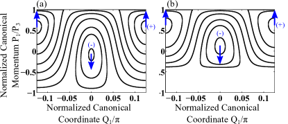
Figure 3: Phase space portrait with normalized phase-mismatch $\Delta\Gamma=0.6\sqrt{P_{3}}$ and (a) $P_{2}=0$ (b) $P_{2}=0.3P_{3}$. Arrows indicate motion of fixed points with increasing $\Delta\Gamma$.

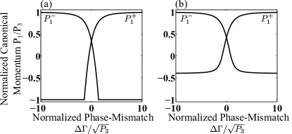
Figure 4: Normalized reduced phase-space canonical momentum for the two stationary states with (a) $P_{2}=0$ (b) $P_{2}=0.3P_{3}$.

III Adiabatic Evolution and Bandwidth

III.1 Adiabatic Evolution

According to classical mechanical theory Arnold_book , an elliptic fixed point will follow an adiabatically varying control parameter, i.e. a parameter that changes slowly compared with the frequencies of periodic orbits around the fixed point. It will be shown how this adiabaticity condition naturally arises from a linearization of the canonical Hamiltonian dynamics, i.e. Eq. 17, about the fixed point Liu_PRL_78 ; Arnold_book , where the adiabatically varying parameter is the phase-mismatch $\Delta\Gamma$. The main result of this work is the derivation of the adiabaticity condition, as will be outlined below.

The linearization procedure of Eq. 17 is detailed in appendix A. It is shown that the nontrivial stationary states correspond to elliptic fixed points, and that

$$\delta P_{1}\approx\frac{1}{\nu}\frac{dP_{1}^{\pm}}{d\xi}sin\left(\nu\xi\right)$$ (24)

where $\delta P_{1}=P_{1}-P_{1}^{\pm}$, i.e. it is the vertical difference between the system point and a fixed point in the $\left(Q_{1},P_{1}\right)$ phase-space. $\nu$ is the frequency of periodic orbits around the fixed point. In the ideal case, the system would be exactly at the stationary state throughout the entire interaction, i.e. $\delta P_{1}=0$. We thus set the nonlinear adiabaticity condition to be

$$r_{nl} \equiv$$

$$\left|\frac{\left[\frac{1}{2}\left(\left|q_{1}\right|^{2}+\left|q_{2}\right|^{2}\right)-\left|q_{3}\right|^{2}\right]-\left[\frac{1}{2}\left(\left|q_{1}^{\pm}\right|^{2}+\left|q_{2}^{\pm}\right|^{2}\right)-\left|q_{3}^{\pm}\right|^{2}\right]}{\frac{1}{2}\left(\left|q_{1}\right|^{2}+\left|q_{2}\right|^{2}\right)+\left|q_{3}\right|^{2}}\right|$$

$$=\left|\frac{\delta P_{1}}{P_{3}}\right|\ll 1$$ (25)

The physical interpretation of $r_{nl}$ is as follows. Each of the two terms in square brackets represents photon flux excess of the low frequency waves over the high frequency waves. The first of these terms is for the state under consideration, while the second is for the stationary state. Therefore, the complete numerator represents the difference in photon flux excess between a given set of waves and the stationary state. The denominator normalizes this quantity by the overall photon flux balance between the three waves.

Using the approximate solution of Eq. 24 for $\delta P_{1}$, this condition becomes

$$\left|\frac{d\left(P_{1}^{\pm}/P_{3}\right)}{d\xi}\right|=\left|\frac{d\left(P_{1}^{\pm}/P_{3}\right)}{d\Delta\Gamma}\frac{d\Delta\Gamma}{d\xi}\right|\ll\nu$$ (26)

which means that in order to maintain adiabaticity, the rate of change of the normalized stationary state photon flux excess in the low frequencies over the high frequencies, $P_{1}^{\pm}/P_{3}$, has to be much slower than the frequency of periodic orbit around the fixed point, as expected from classical mechanical theory. Eq. 26 is the main result of this work. For the special case of $\left|q_{1}\right|^{2}=\left|q_{2}\right|^{2}$ and $\Delta\Gamma=0$, this inequality leads to

$$\frac{2}{\sqrt{27}}\frac{1}{P_{3}}\left|\frac{d\Delta\Gamma}{d\xi}\right|\ll 1$$ (27)

Adiabaticity can thus be more closely satisfied when the overall intensity is higher (which increases the overall photon flux $P_{3}$) and when the rate of change of the phase-mismatch is lower.

Having established that the system can adiabatically follow changes in the phase-mismatch $\Delta\Gamma$, we consider the special case where the system is prepared in a nontrivial stationary state of Eq. 22, $\left|\Delta\Gamma\right|\gg\sqrt{2P_{3}}$ at the beginning and end of the interaction, and $\Delta\Gamma$ ends with a sign opposite to the one it started with. Clearly, from Fig. 1, when $\left|q_{1}\right|^{2}=\left|q_{2}\right|^{2}$ the adiabatic interaction would result in a complete energy transfer from the two lower frequencies, $\omega_{1}$ and $\omega_{2}$, to the high frequency, $\omega_{3}$. Since it was established that $P_{1}^{+}\left(\Delta\Gamma/\sqrt{P_{3}}\right)=P_{1}^{-}\left(-\Delta\Gamma/\sqrt{P_{3}}\right)$, we will concentrate on adiabatic following of $P_{1}^{-}$, where it is readily understood that everything applies to $P_{1}^{+}$ upon reversal of the chirp direction.

In order to demonstrate adiabatic evolution, Eq. 1 were solved numerically for three different cases. The results are displayed in Fig. 5. In this figure, the dashed curves correspond to the minus stationary state, calculated using Eq. 22. $r_{nl}$ in (c), (f) and (i) was calculated using Eq. 26. In all three cases the system started in the minus state. In each case the phase-mismatch chirp rate was different, i.e. $\Delta\Gamma$ was always linearly chirped from $-10\sqrt{P_{3}}$ to $10\sqrt{P_{3}}$, but the interaction length was varied. In the first case, shown in Fig. 5a-c, the normalized interaction length was $\Delta\xi\sqrt{P_{3}}=1$. Clearly in this case the system does not follow the stationary state. Correspondingly, the adiabatic condition is not satisfied, as $r_{nl}$ reaches a value much greater than $1$. In the second case, displayed in Fig. 5d-f, $\Delta\xi\sqrt{P_{3}}=10$. In this case the stationary state is more closely followed, yet only to a limited extent. This is also reflected in the fact that $r_{nl}$ reaches $0.85$. Note that the area of departure from the stationary state in Fig. 5d and e corresponds to the area where $r$ increases toward $0.85$ in Fig. 5f. Finally, in the third case, $\Delta\xi\sqrt{P_{3}}=100$. Fig. 5g-i show that in this case the the stationary state is very closely followed, and $r_{nl}\ll 1$ throughout the entire interaction.

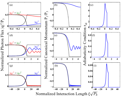
Figure 5: Numerical solutions of Eq. 1 with $\left|q_{1}\right|^{2}=\left|q_{2}\right|^{2}$. $\Delta\Gamma$ is linearly chirped from $-10\sqrt{P_{3}}$ to $10\sqrt{P_{3}}$. The system always starts in the minus stationary state. The normalized interaction length is (a-c) $\Delta\xi\sqrt{P_{3}}=1$ (d-f) $\Delta\xi\sqrt{P_{3}}=10$ (g-i) $\Delta\xi\sqrt{P_{3}}=100$. The dashed curves correspond to the minus stationary state calculated using Eq. 22. The nonlinear adiabatic condition $r_{nl}$ in (c), (f) and (i) was calculated using Eq. 26. Only the bottom row, in which $r_{nl}\ll 1$, satisfies the adiabatic condition.

In the general case of $\left|q_{1}\right|^{2}\neq\left|q_{2}\right|^{2}$, i.e. $P_{2}\neq 0$, $P_{1}$ will go from $P_{3}$ to $2\left|P_{2}\right|-P_{3}$ for increasing $\Delta\Gamma$, when the adiabaticity condition is met. This means that energy will be transferred from the two low frequencies $\omega_{1}$ and $\omega_{2}$ to the high frequency $\omega_{3}$, until one of the two low frequencies is depleted. A numerical simulation of such a case is displayed in Fig. 6, where $P_{2}=0.3P_{3}$. As seen in Fig. 6a, energy is adiabatically transferred from the low frequencies to the high frequency until none is left at $\omega_{2}$. From that point on, the three waves intensities remain essentially unchanged. Fig. 6b shows the corresponding value of $P_{1}/P_{3}$, which indeed goes from $1$ to $\left(2\left|P_{2}\right|-P_{3}\right)/P_{3}=-0.4$, as expected.

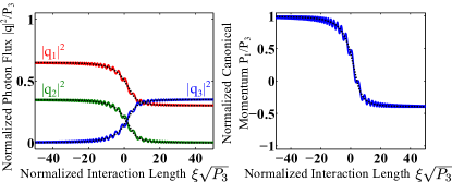
Figure 6: Numerical solution of Eq. 1 with the same parameters as in Fig. 5g, except that $P_{2}=0.3P_{3}$. The dashed curves correspond to the minus stationary state.

A special case of the nonlinear adiabatic evolution is the case of constant pump approximation Suchowski_PRA_78 ; Suchowski_OE_17 ; Suchowski_APB_105 ; Moses_OL_37 ; Porat_OL_35_1590 ; Porat_OE_20 ; Porat_JOSAB_29 ; Porat_APL ; Rangelov_PRA_85 , where the dynamics becomes linear. In this scenario, one of the three waves (the pump wave) was taken to be much more intense than the other two waves, while another wave was assumed to start with no energy. Under the assumption that the effect of the interaction on the pump wave is negligible, the remaining two waves form a linear dynamical system, to which the linear adiabatic theorem applies. As a result, energy would flow from one interacting wave to to other. Such a situation was simulated here as well, without making the fixed pump approximation, with the results displayed in Fig. 7. In this case, the input pump-to-signal ratio was $\left|q_{2}\left(0\right)\right|^{2}/\left|q_{1}\left(0\right)\right|^{2}=100$ and $\left|q_{3}\left(0\right)\right|^{2}=0$. Fig. 7a shows that all of the photon flux was transferred from $\omega_{1}$ to $\omega_{3}$, with equal contribution from $\omega_{2}$ as evident from the inset. This corresponds completely to the above description, i.e. the adiabatic interaction took place until the $\omega_{1}$ wave was depleted. Fig. 7b shows that $P_{1}/P_{3}$ traveled from $1$ to $2\left|P_{2}\right|-P_{3}=0.96$, as expected.

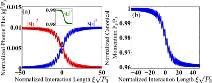
Figure 7: Numerical solution of Eq. 1 with the same parameters as in Fig. 5g, but assuming a strong pump at $\omega_{2}$, a weak signal at $\omega_{1}$ and no input energy at $\omega_{3}$, i.e. the approximate linear dynamics regime. The dashed curves correspond to the minus stationary state. The inset of (a) shows $\left|q_{2}\right|^{2}/P_{3}$ and has the same horizontal axis.

Finally, we note that a trivial stationary state does not correspond to an elliptic fixed point in the $\left(Q_{1},P_{1}\right)$ phase space (see appendix A), so it would not perform adiabatic following due to changing phase-mismatch. This of course can be expected on physical grounds, as we do not expect the intensity of the only present frequency to be affected by changes in phase-mismatch between it and absent frequencies. Interestingly, for the case where $\left|q_{1}\right|^{2}=\left|q_{2}\right|^{2}$, each of the two nontrivial stationary states can actually follow the adiabatically-varying phase-mismatch into a trivial stationary state with $\left|q_{1}\right|^{2}=\left|q_{2}\right|^{2}=0$, as evident from Fig. 1 and 4.

To summarize this section, adiabatic following can be obtained when the system is prepared to be near a nontrivial stationary state, i.e. such that $\delta P_{1}\ll P_{3}$, and the rate of change of the scaled phase mismatch $\Delta\Gamma$ is sufficiently small for the given overall photon flux balance $P_{3}$, as prescribed by Eq. 26. If $\Delta\Gamma$ changes monotonically, changing signs from beginning to end, and $\left|\Delta\Gamma\right|\gg\sqrt{P_{3}}$ at the beginning and end of the interaction, the system will evolve adiabatically from $P_{1}=P_{3}$ to $P_{1}=2\left|P_{2}\right|-P_{3}$, or vice versa. The former corresponds to upconversion, which ends when one of the two low frequency waves is depleted (the one that started with the lower photon flux). The latter corresponds to downconversion, which continues until the high frequency wave is depleted. In the special case where $P_{2}=0$, the system can only evolve from $P_{1}=P_{3}$ to $P_{1}=-P_{3}$, but not in the reverse direction, since $P_{1}=-P_{3}$ is a trivial stationary state that does not correspond to an elliptic fixed point in the $\left(Q_{1},P_{1}\right)$ reduced phase space.

As a final note, we would like to suggest that the same method can be applied to frequency-cascaded and spatially-simultaneous TWM processes or higher-order nonlinear adiabatic processes. For example, four wave mixing has also been put into canonical Hamiltonian structure, and symmetries, corresponding conservation laws and stationary states have been identified Amiranashvili_PRA_82 . Optical fiber tapering can be used to facilitate adiabatic evolution. A detailed analysis will be carried out elsewhere.

III.2 Bandwidth

Adiabatic TWM processes have numerically been shown to be robust against changes in various parameters, e.g. wavelength and temperature Suchowski_PRA_78 ; Suchowski_OE_17 ; Suchowski_APB_105 ; Moses_OL_37 ; Porat_OL_35_1590 ; Porat_APL ; Rangelov_PRA_85 , which are manifested in changes in the phase-mismatch. This robustness stems from the fact that $\Delta\Gamma$ is swept along a large range of values, so a wide range of physical conditions can result in $\Delta\Gamma$ within the range that satisfies the conditions for adiabatic evolution.

An estimate of the bandwidth will now be given and demonstrated. First, we define the conversion efficiency for following the minus state with increasing $\Delta\Gamma$,

$$\eta\equiv\frac{P_{3}}{2\left(\left|P_{2}\right|-P_{3}\right)}\left(\frac{P_{1}}{P_{3}}-1\right)$$ (28)

Under this definition, $\eta\left(P_{1}=P_{3}\right)=0$ and $\eta\left(P_{1}=\left|P_{2}\right|-P_{3}\right)=1$. The full width at half maximum of $\eta$ is estimated to be (see appendix B for details)

$$\Delta\Gamma_{BW}=\Delta\Gamma\left(\Delta\xi/2\right)-\Delta\Gamma\left(-\Delta\xi/2\right)$$ (29)

The estimated bandwidth is therefore independent of the intensities of the interacting waves, as it depends only on the chirp range of $\Delta\Gamma$.

The conversion efficiency $\eta$ for $P_{2}=0$ and $P_{2}=0.3P_{3}$ is depicted in Fig. 8a and 8b, respectively, vs. the normalized phase mismatch at the center of the interaction medium. In this simulation, the chirp rate and interaction length were kept constant. The vertical dashed lines indicate the locations where the estimated efficiency is $\frac{1}{2}$, established by introducing $P_{1}^{-}=\left|P_{2}\right|$ into Eq. 11. For $P_{2}=0$ and $P_{2}=0.3P_{3}$, the simulated bandwidth $\Delta\Gamma_{BW}/\sqrt{P_{3}}$ is $19.46$ and $19.7$, respectively.. For both cases, the estimated bandwidth is $\Delta\Gamma_{BW}/\sqrt{P_{3}}=20$, which is within $3\%$ of the numerical results.

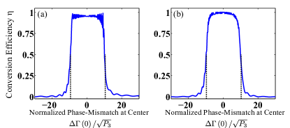
Figure 8: Numerically calculated conversion efficiency with (a) $P_{2}=0$ and (b) $P_{2}=0.3P_{3}$, and all other parameters the same as in Fig. 5g, for various values of the normalized phase-mismatch at the center of the interaction medium, $\Delta\Gamma\left(0\right)/\sqrt{P_{3}}$. The chirp rate and interaction length were kept constant. The dashed lines indicate the values of $\Delta\Gamma\left(0\right)/\sqrt{P_{3}}$ where the estimation yields $\eta=\frac{1}{2}$.

For a given chirped phase-mismatch, the bandwidth will depend on intensity where intensity determines whether the adiabatic evolution conditions are satisfied. On the one hand, when the intensity is too low to satisfy the adiabatic condition of Eq. 26, the efficiency will always be low. Shifting of $\Delta\Gamma\left(0\right)$ from $\sim 0$ will more quickly deteriorate efficiency than when adiabatic following takes place, thus the bandwidth is expected to be lower. On the other hand, when the intensity is high enough, $\left|\Delta\Gamma\right|\gg\sqrt{P_{3}}$ will never be satisfied, so $P_{1}$ will not be close to $P_{3}$ at the beginning of the interaction. However, in this case adiabatic following is still maintained to some extent, i.e. the motion of $P_{1}^{-}$ is still slow enough to satisfy Eq. 26, so $P_{1}$ can follow it. $P_{1}$ will thus orbit the adiabatically moving fixed point with a large orbit diameter. This will cause the efficiency to oscillate rapidly for various $\Delta\Gamma\left(0\right)$, so a useful definition of bandwidth is difficult to find. These phenomena are demonstrated numerically in section IV.

Finally we note that the bandwidth estimation of Eq. 29 is valid not only for following the minus state, but whenever the requirements of adiabatic following are satisfied, i.e. $P_{1}\approx P_{3}$ or $P_{1}\approx 2\left|P_{2}\right|-P_{3}$ at the beginning of the interaction, $\Delta\Gamma$ chirped such that it changes sign from beginning to end, $\left|\Delta\Gamma\right|\gg\sqrt{P_{3}}$ at the beginning and end of the interaction and Eq. 26 is satisfied throughout the entire process (the details can be found in appendix B). It follows that the rest of the discussion, regarding intensity too low or too high to satisfy all of the aforementioned requirements, is also true for all cases, not just those related to $P_{1}^{-}$ and increasing $\Delta\Gamma$.

IV Numerical Simulations

In this section, the results of numerical simulations of Eq. 1 will be shown, with physical dimensions rather than normalized units. It will be demonstrated that fully nonlinear, efficient and wideband adiabatic frequency conversion can readily be applied in a wide variety of physically available configurations, using QPM. In all of the simulations presented below, the nonlinear medium was taken to be a $40mm$ long $LiNbO_{3}$ crystal with $\chi^{\left(2\right)}=50pm/V$ Shoji_JOSAB_14 . The Sellmeier equations of Gayer et al. Gayer_APB_91 were used to account for dispersion.

SFG is addressed first. In this simulation, $\lambda_{2}=1064.5nm$ and $\lambda_{1}$ is tuned in the range $1450-1650nm$, which yields $614<\lambda_{3}<647nm$. The input intensities of the two low frequencies are chosen such that they have the same photon flux when $\lambda_{1}=1550nm$, and the sum frequency wave at $\lambda_{3}$ was always taken to start with no energy. The simulated crystal had chirped QPM modulation, with a local period starting at $11.52\mu m$ and ending at $11.79\mu m$. This correspond to $\Delta\Gamma$ that goes from $-3\sqrt{P_{3}}$ to $3\sqrt{P_{3}}$ for a total input intensity of $200MW/cm^{2}$ when $\lambda_{1}=1550nm$.

Fig. 9a shows the intensities of the three waves along the crystal when $\lambda_{1}=1550nm$ and the total input intensity was $200MW/cm^{2}$. As expected, energy is very efficiently transferred from the two low frequencies to the high frequency. The photon flux conversion efficiency $\eta$, defined by Eq. 28, is $0.93$. Fig. 9b shows the conversion efficiency as a function of input wavelength, for several input intensities. For input intensities of $2$ and $200MW/cm^{2}$, the maximum efficiency was $0.11$ and $0.97$, with bandwidths of $54.2$ and $55.5nm$, respectively. These results correspond to the analysis given in subsection III.2: the significant increase of efficiency, and the slight increase in bandwidth, with intensity, is related to improvement in the satisfaction of the adiabatic condition of Eq. 26. For input intensity of $20000MW/cm^{2}$, the efficiency performs oscillations across the $\lambda_{1}$ tuning range, as predicted, due to the fact that the system point is orbiting the fixed point from a relatively large distance.

Figure 9: SFG simulation results: (a) Intensities of the three waves along the crystal for input wavelength $\lambda_{1}=1550nm$ and input intensity $200MW/cm^{2}$ (b) Conversion efficiency vs. $\lambda_{1}$ for different input intensities, which are indicated in units of $MW/cm^{2}$.

SHG can be considered as a special case of SFG with $\left|q_{1}\right|^{2}=\left|q_{2}\right|^{2}$, where, additionally, $\omega_{1}=\omega_{2}$. A simulation was conducted for this case well, where the QPM period was chirped from $18.83\mu m$ to $19.44\mu m$, once again corresponding to $\Delta\Gamma$ that goes from $-3\sqrt{P_{3}}$ to $3\sqrt{P_{3}}$ for input intensity of $200MW/cm^{2}$ when $\lambda_{1}=1550nm$ . All other parameters were the same as before. The outcome is displayed in Fig. 10, showing results similar to the case of SFG with $\omega_{1}\neq\omega_{2}$. For input intensity of $200MW/cm^{2}$ , at $\lambda_{1}=1550nm$ the conversion efficiency was 0.96, and the bandwidth was $42nm$.

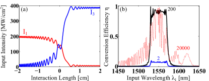
Figure 10: SHG simulation results: (a) Intensities of the two waves along the crystal for input wavelength $\lambda_{1}=1550nm$ and input intensity $200MW/cm^{2}$ (b) Conversion efficiency vs. $\lambda_{1}$ for different input intensities, which are indicated in units of $MW/cm^{2}$.

Difference frequency generation (DFG) is the case where energy is transferred from the high frequency to the two low frequencies. In the DFG simulations $\lambda_{3}=1064.5nm$ and $\lambda_{2}$ was tuned over $1400-1800nm$, which generates $2605<\lambda_{1}<4442nm$ (consistent with our convention that $\omega_{1}<\omega_{2}<\omega_{3}$). The QPM period was chirped from $29.86$ to $30.86\mu m$, and here also $\Delta\Gamma$ goes from $-3\sqrt{P_{3}}$ to $3\sqrt{P_{3}}$ for input intensity of $200MW/cm^{2}$ when $\lambda_{2}=1550nm$ (the other low frequency, $\omega_{1}$, always starts with no energy). All other parameters were the same as before. In Fig. 11a it is seen that energy is efficiently transferred from the high frequency to the two low frequencies, for the case of $\lambda_{2}=1550nm$ and input intensity of $200MW/cm^{2}$. Note that in this case the system follows the plus stationary state ($P_{1}$ starts out negative). The conversion efficiency is thus $1-\eta$, which corresponds to the degree of depletion of the high frequency. For the case presented in Fig. 11a, the efficiency is 0.95. Fig. 11b displays the conversion efficiency vs. $\lambda_{2}$ for different input intensities, showing the same dependence as in the previous cases. For input intensity of $200MW/cm^{2}$, the bandwidth was $212nm$.

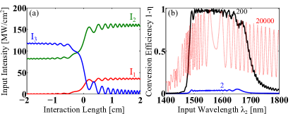
Figure 11: DFG simulation results: (a) Intensities of the three waves along the crystal for input wavelength $\lambda_{2}=1550nm$ and input intensity $200MW/cm^{2}$ (b) Conversion efficiency vs. $\lambda_{2}$ for different input intensities, which are indicated in units of $MW/cm^{2}$.

The special case of DFG where the input intensity of the high frequency is much higher than that of the input low frequency ($\omega_{2}$ in this case), is commonly denoted OPA. In the OPA simulation, the QPM structure was designed such that $\Delta\Gamma$ goes from $-2\sqrt{P_{3}}$ to $2\sqrt{P_{3}}$ when $\lambda_{2}=1550nm$ and the input intensity is $400MW/cm^{2}$. Also, the $\omega_{2}$ input intensity was 20 times lower than the $\omega_{3}$ input intensity. The resulting QPM period was chirped over $29.98-30.85\mu m$. All other parameters are the same as for the DFG simulation. Fig. 12a shows the intensities of the three waves along the crystal for $\lambda_{2}=1550nm$ and input intensity of $400MW/cm^{2}$. As before, energy is seen to efficiently transfer from the high frequency to the two low frequencies, resulting in conversion efficiency of 0.97. From start to end, the intensity at $\omega_{2}$ was amplified by a factor of 13.6. In Fig. 11b the conversion efficiency is plotted vs. $\lambda_{2}$ for different input intensities, with the same behavior as noted above. A detailed numerical investigation of adiabatic OPA has been conducted by Phillips et al. Phillips_OL_35 .

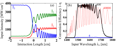
Figure 12: OPA simulation results: (a) Intensities of the three waves along the crystal for input wavelength $\lambda_{2}=1550nm$ and input intensity $200MW/cm^{2}$ (b) Conversion efficiency vs. $\lambda_{2}$ for different input intensities, which are indicated in units of $MW/cm^{2}$.

The range of parameters used above shows that adiabatic TWM can readily be used with nanosecond to picosecond pulsed lasers in bulk media or continuous-wave lasers in guided structures (e.g. QPM waveguides Hum_CRP_8 ). Shorter pulses could be stretched, converted and compressed again Suchowski_PRA_78 ; Suchowski_OE_17 ; Suchowski_APB_105 ; Moses_OL_37 .

The combination of broad bandwidth and intensity dependence of efficiency suggests another application of fully nonlinear TWM - cleaning the unwanted pedestal of intense ultra-short pulses Saltiel_OL_24 ; Ganany_APL_94 . This could be performed using two QPM crystals, as follows. First, the input beam should be linearly polarized at 45 degrees to two of the crystals optical axes, namely the ordinary and extraordinary axes. In this manner, half of the input energy would be at the ordinary polarization, and half at the extraordinary polarization. We denote these frequency and polarization components $\omega_{o}$ and $\omega_{e}$, respectively. The first crystal will perform cross-polarized adiabatic SHG of the extraordinary polarization, i.e. $\omega_{e}+\omega_{e}\rightarrow 2\omega_{o}$. Since conversion efficiency depends on intensity, the high-power parts of the pulse will be more efficiently converted than the low-power parts. Therefore, after the first crystal, the $\omega_{e}$ wave contains the remaining low-power parts of the pulse. These are eliminated by placing a polarizer, aligned along the ordinary axis, following the first crystal. After the polarizer, we are left with the generated $2\omega_{o}$ wave and the original (uncleaned) $\omega_{o}$ wave. These waves now enter the second crystal, which performs the degenerate cross-polarized DFG process $2\omega_{o}-\omega_{o}\rightarrow\omega_{e}$. Once again, the process favors the high-power parts of the pulse at $\omega_{o}$. Passing the output through a polarizer aligned along the extraordinary wave will eliminate the residual low-power at $\omega_{o}$ as well as $2\omega_{o}$, leaving only the cleaned pulse at $\omega_{e}$.

V Conclusion

Adiabatic TWM with fully nonlinear dynamics was put on a firm physical basis by rigorous analysis, detailing the conditions for obtaining adiabatic evolution. Just as the adiabatic TWM in the linear dynamics regime was developed from an analogy with linear quantum systems Suchowski_PRA_78 ; Suchowski_OE_17 , the method used here also follows, in general terms, an analysis of adiabatic evolution of nonlinear quantum systems Pu_PRL_98 ; Liu_PRL_78 ; Meng_PRA_78 . Furthermore, the nonlinear adiabatic condition was determined, and an estimation of the bandwidth of adiabatic TWM processes was derived and shown to be consistent with numerical results. In addition, numerical simulations were used to demonstrated fully nonlinear adiabatic frequency conversion in several configurations attainable with current technology. Specifically, adiabatic SFG, SHG, DFG and OPA were all shown to be efficient over a wide band of input frequencies, using intensities characteristic of nanosecond pulses in bulk interactions or continuous-wave lasers in guided structures. It was also explained how adiabatic TWM could be used to facilitate efficient pulse cleaning. Finally, it was suggested that adiabatic evolution of frequency-cascaded and spatially-simultaneous TWM processes or higher order nonlinear processes, such as four wave mixing, can also be treated using the same method.

Appendix A: Linearization of the Canonical Hamiltonian Dynamics

This appendix details the linearization procedure that was utilized to obtain Eq. 24. Linearization of Eq. 17, i.e. of $\partial H/\partial P_{1}$ and $\partial H/\partial Q_{1}$, can be accomplished in a single step, by approximating the Hamiltonian $H$ with a Taylor expansion around a fixed point $\left(Q_{1}^{\pm},P_{1}^{\pm}\right)$ up to second order:

$$H\left(Q_{j},P_{j}\right)\approx H\left(Q_{j}^{\pm},P_{j}^{\pm}\right)+\left.\frac{\partial^{2}H}{\partial Q_{1}^{2}}\right|_{\left(Q_{j}^{\pm},P_{j}^{\pm}\right)}\delta Q_{1}+\left.\frac{\partial^{2}H}{\partial P_{1}^{2}}\right|_{\left(Q_{j}^{\pm},P_{j}^{\pm}\right)}\delta P_{1}$$ (A1)

where $\delta Q_{1}=Q_{1}-Q_{1}^{\pm}$, $\delta P_{1}=P_{1}-P_{1}^{\pm}$, and we have used Eq. 20, and also $\left.\partial^{2}H/\partial Q_{1}P_{1}\right|_{\left(Q_{j}^{\pm},P_{j}^{\pm}\right)}=0$. Substituting the approximate Hamiltonian in Eq. 17 leads to the linear equations of motion

$$\frac{d}{d\xi}\begin{bmatrix}\delta P_{1}\\ \delta Q_{1}\end{bmatrix} = \begin{bmatrix}0&-\left.\frac{\partial^{2}H}{\partial Q_{1}^{2}}\right|_{Q_{1}^{\pm},P_{1}^{\pm}}\\ \left.\frac{\partial^{2}H}{\partial P_{1}^{2}}\right|_{Q_{1}^{\pm},P_{1}^{\pm}}&0\end{bmatrix}\begin{bmatrix}\delta P_{1}\\ \delta Q_{1}\end{bmatrix}-\begin{bmatrix}\frac{dP_{1}^{\pm}}{d\xi}\\ \frac{dQ_{1}^{\pm}}{d\xi}\end{bmatrix}$$

Note that the variation in $\Delta\Gamma$ causes $P_{1}^{\pm}$ to be $\xi$dependent, and thus $dP_{1}^{\pm}/d\xi$ functions as a source term in Eq. LABEL:eq:linearized_dynamics, whereas $dQ_{1}^{\pm}/d\xi=0$ (see Eq. 21). We solve for $\delta P_{1}$, assuming an initial condition of $\delta P_{1}=0$, by diagonalizing the coupling matrix, which yields

$$\delta P_{1}=\int_{0}^{\xi}cos\left[\nu\left(\xi-\xi^{\prime}\right)\right]\frac{dP_{1}^{\pm}}{d\xi^{\prime}}d\xi^{\prime}$$ (A3)

where

$$\nu=\sqrt{\left.\frac{\partial^{2}H}{\partial Q_{1}^{2}}\right|_{Q_{1}^{\pm},P_{1}^{\pm}}\left.\frac{\partial^{2}H}{\partial P_{1}^{2}}\right|_{Q_{1}^{\pm},P_{1}^{\pm}}}$$ (A4)

is the magnitude of each of the two imaginary eigenvalues of the coupling matrix $\pm i\nu$. The nontrivial stationary states fixed points are thus elliptic, where $\nu$ is the frequency of periodic orbits around the fixed point. Since it is assumed that the system is near an elliptic fixed point, this frequency is large compared to all other rates of variation, so the most significant contribution to the integral of Eq. A3 comes from $\xi\approx\xi^{\prime}$. We can therefore approximate $\delta P_{1}$ by taking $dP_{1}/d\xi^{\prime}$ at $\xi^{\prime}=\xi$, which can then be taken outside of the integral, yielding

$$\delta P_{1}\approx\frac{1}{\nu}\frac{dP_{1}^{\pm}}{d\xi}sin\left(\nu\xi\right)$$ (A5)

which was used for Eq. 24.

Finally, we note that the discussion above referred to a nontrivial stationary state. Repeating the same analysis for a trivial stationary state, for which $H=-\left(\Delta\Gamma/8\right)\left(P_{1}+3P_{3}\right)$, yields a matrix with two zero eigenvalues in Eq. LABEL:eq:linearized_dynamics. Therefore, a trivial stationary state does not correspond to an elliptic fixed point in the $\left(Q_{1},P_{1}\right)$ phase space.

Appendix B: Bandwidth Estimation

An estimate of the full width at half maximum of the conversion efficiency $\eta$ (see Eq. 28) will now developed. As noted in subsection III.2, $\eta\left(P_{1}=P_{3}\right)=0$ and $\eta\left(P_{1}=\left|P_{2}\right|-P_{3}\right)=1$. Furthermore, $\eta\left(P_{1}=\left|P_{2}\right|\right)=\frac{1}{2}$, i.e. $\eta=\frac{1}{2}$ when $P_{1}$ is exactly half way between $P_{3}$ and $2\left|P_{2}\right|-P_{3}$. If $P_{1}$ starts at $P_{3}$ and follows $P_{1}^{-}$, it is expected that $P_{1}$ will end up at $\left|P_{2}\right|$, i.e. half way to $2\left|P_{2}\right|-P_{3}$, if the stationary state fixed point $P_{1}^{-}$ has traveled the same distance. Assuming a very large chirp range, such that $P_{1}^{-}$ always starts near $P_{3}$ or ends near $2\left|P_{2}\right|-P_{3}$ (or both), there are two cases in which this may happen: (i) $P_{1}^{-}$ starts near $P_{3}$ and ends up at $\left|P_{2}\right|$ (ii) $P_{1}^{-}$ starts at $\left|P_{2}\right|$ and ends near $2\left|P_{2}\right|-P_{3}$. In the first case the estimation is more accurate, since $P_{1}$ starts near $P_{1}^{-}$ and will thus follow it as expected from the above theory. In the second case, $P_{1}$ starts near $P_{3}$ while $P_{1}^{-}$ starts at $\left|P_{2}\right|$, i.e. they are not near, so $\delta P_{1}\ll P_{3}$ is not satisfied. Still, as a first order approximation, we can expect $P_{1}$ to traverse a path of similar length to that of $P_{1}^{-}$. Thus, in the first case the condition $P_{1}^{-}=\left|P_{2}\right|$ is satisfied by $\Delta\Gamma$ at the end of the interaction, while at the second case it is satisfied at the start. The difference between these two values of $\Delta\Gamma$ is, by definition, the chirp range, i.e. the bandwidth is estimated to be

$$\Delta\Gamma_{BW}=\Delta\Gamma\left(\Delta\xi/2\right)-\Delta\Gamma\left(-\Delta\xi/2\right)$$ (B1)

The above analysis assumes following of the minus state with increasing $\Delta\Gamma$, however it applies to the general case of adiabatic following. First, when the minus state is followed with decreasing $\Delta\Gamma$, the efficiency is simply $1-\eta$, so the two conditions for $\eta=\frac{1}{2}$ are clearly the same for $1-\eta=\frac{1}{2}$. Furthermore, following the plus state is the same as following the minus state with the opposite chirp direction, so once again the same conditions apply. The estimation is therefore valid whenever the requirements of adiabatic following are satisfied, i.e. $P_{1}\approx P_{3}$ or $P_{1}\approx 2\left|P_{2}\right|-P_{3}$ at the beginning of the interaction, $\Delta\Gamma$ chirped such that it changes sign from beginning to end, $\left|\Delta\Gamma\right|\gg\sqrt{P_{3}}$ at the beginning and end of the interaction and the condition of Eq. 26.

VI Acknowledgments

The authors would like to thank Dr. Haim Suchowski for fruitful discussions.

References

- (1) R. W. Boyd, Nonlinear Optics, ed. (Academic Press, 2008).
- (2) J. A. Armstrong, N. Bloembergen, J. Ducuing, and P. S. Pershan, “Interactions between light waves in a nonlinear dielectric,” Phys. Rev. 127, 1918-1939 (1962).
- (3) D. S. Hum and M. M. Fejer, “Quasi-phasematching,” C. R. Physique 8, 180–198 (2007).
- (4) H. Suchowski, D. Oron, A. Arie, and Y. Silberberg, “Geometrical representation of sum frequency generation and adiabatic frequency conversion,” Phys. Rev. A 78, 063821 (2008).
- (5) H. Suchowski, V. Prabhudesai, D. Oron and Y. Silberberg, “Robust adiabatic sum frequency conversion,” Opt. Express 17, 12731-12740 (2009).
- (6) H. Suchowski, B. D. Bruner, A. Ganany-Padowicz, I. Juwiler, A. Arie, and Y. Silberberg, “Adiabatic frequency conversion of ultrafast pulses,” Appl. Phys. B 105, 697-702 (2011).
- (7) J. Moses, H. Suchowski, and F. X. K rtner, “Fully efficient adiabatic frequency conversion of broadband Ti:sapphire oscillator pulses,” Opt. Lett. 37, 1589-1591 (2012).
- (8) G. Porat, H. Suchowski, Y. Silberberg and A. Arie, “Tunable upconverted optical parametric oscillator with intracavity adiabatic sum-frequency generation,” Opt. Lett. 35, 1590-1592 (2010).
- (9) G. Porat, Y. Silberberg, A. Arie, and H. Suchowski, “Two photon frequency conversion,” Opt. Express 20, 3613-3619 (2012).
- (10) G. Porat and A. Arie, “Efficient two-process frequency conversion through a dark intermediate state,” J. Opt. Soc. Am. B 29, 2901-2909 (2012).
- (11) G. Porat and A. Arie, “Efficient broadband frequency conversion via simultaneous three wave mixing processes,” Appl. Phys. Lett., submitted.
- (12) A. A. Rangelov and N. V. Vitanov, “Broadband sum-frequency generation using cascaded processes via chirped quasi-phase-matching,” Phys. Rev. A 85, 045804 (2012).
- (13) A. Messiah, Quantum Mechanics (North Holland, 2005).
- (14) N. B. Baranova, M. A. Bolshtyanskiĭ, and B. Ya Zel’dovich, “Adiabatic energy transfer from a pump wave to its second harmonic,” Quantum Electronics 25, 638-640 (1995).
- (15) C. R. Phillips and M. M. Fejer, “Efficiency and phase of optical parametric amplification in chirped quasi-phase-matched gratings,” Opt. Lett. 35, 3093-3095 (2010).
- (16) C. R. Phillips and M. M. Fejer, “Adiabatic optical parametric oscillators: steady-state and dynamical behavior,” Opt. Express 20, 2466-2482 (2012).
- (17) M. D. Crisp, “Adiabatic-Following Approximation,” Phys. Rev. A 8, 2128-2135 (1973).
- (18) G. G. Luther, M. S. Alber, J. E. Marsden, and J. M. Robbins, “Geometric analysis of optical frequency conversion and its control in quadratic nonlinear media,” J. Opt. Soc. Am. B 17, 932-941 (2000).
- (19) R. P. Feynman, F. L. Vernon, JR., and R. W. Hellwarth, “Geometrical Representation of the Schr dinger Equation for Solving Maser Problems,” J. Appl. Phys. 28, 49-52 (1957).
- (20) S. Longhi, “Third-harmonic generation in quasi-phase-matched media with missing second harmonic,” Opt. Lett. 32, 1791-1793 (2007).
- (21) H. Pu, P. Maenner, W. Zhang, and H. Y. Ling, “Adiabatic Condition for Nonlinear Systems,” Phys. Rev. Lett. 98, 050406 (2007).
- (22) O. Yaakobi, L. Caspani, M. Clerici, F. Vidal, and R. Morandotti, “Complete energy conversion by autoresonant three-wave mixing in nonuniform media,” Opt. Express 21, 1623-1632 (2013).
- (23) J. Liu, B.Wu, Q, Niu, “Nonlinear Evolution of Quantum States in the Adiabatic Regime,” Phys. Rev. Lett. 90, 170404 (2003).
- (24) S. Meng, L. Fu, and J. Liu, “Adiabatic fidelity for atom-molecule conversion in a nonlinear three-level system,” Phys. Rev. A 78, 053410 (2008).
- (25) X. Zhou, Y. Zhang, Z. Zhou, and G. Guo, “Adiabatic evolution in nonlinear systems with degeneracy,” Phys. Rev. A 81, 043614 (2010).
- (26) V. I. Arnol’d, Mathematical Methods of Classical Mechanics (Springer-Verlag, 1978).
- (27) C. J. McKinstrie and X. D. Cao, “Nonlinear detuning of three-wave interactions,” J. Opt. Soc. Am. B 10, 898-912 (1993).
- (28) S. Trillo, S. Wabnitz, R. Chisari, and G. Cappellini, “Two-wave mixing in a quadratic nonlinear medium: bifurcations, spatial instabilities, and chaos,” Opt. Lett. 17, 637-639 (1992).
- (29) A. E. Kaplan, “Eigenmodes of wave mixings: cross-induced second-order nonlinear refraction,” Opt. Lett. 18, 1223-1225 (1993).
- (30) Sh. Amiranashvili and A. Demircan, “Hamiltonian structure of propagation equations for ultrashort optical pulses,” Phys. Rev. A 82, 013812 (2010).
- (31) I. Shoji, T. Kondo, A. Kitamoto, M. Shirane, and R. Ito, “Absolute scale of second-order nonlinear-optical coefficients,” J. Opt. Soc. Am. B 14, 2268-2294 (1997).
- (32) O. Gayer, Z. Sacks, E. Galun, and A. Arie, “Temperature and wavelength dependent refractive index equations for MgO-doped congruent and stoichiometric ,” Appl. Phys. B 91, 343-348 (2008).
- (33) S. Saltiel and Y. Deyanova, “Polarization switching as a result of cascading of two simultaneously phase-matched quadratic processes,” Opt. Lett. 24, 1296-1298 (1999).
- (34) A. Ganany-Padowicz, I. Juwiler, O. Gayer, A. Bahabad, and A. Arie, “All-optical polarization switch in a quadratic nonlinear photonic quasicrystal,” Appl. Phys. Lett. 94, 091108 (2009).