UNVEILING THE DETAILED DENSITY AND VELOCITY STRUCTURES OF THE PROTOSTELLAR CORE B335

Abstract

We present an observational study of the protostellar core B335 harboring a low-mass Class 0 source. The observations of the ${\rm H^{13}CO^{+}}(J=1$–$0)$ line emission were carried out using the Nobeyama 45 m telescope and Nobeyama Millimeter Array. Our combined image of the interferometer and single-dish data depicts detailed structures of the dense envelope within the core. We found that the core has a radial density profile of $n(r)\propto r^{-p}$ and a reliable difference in the power-law indices between the outer and inner regions of the core: $p\approx 2$ for $r\gtrsim 4000\,{\rm AU}$ and $p\approx 1.5$ for $r\lesssim 4000\,{\rm AU}$. The dense core shows a slight overall velocity gradient of $\sim 1.0\,{\rm km\,s^{-1}}$ over the scale of $20{,}000\,{\rm AU}$ across the outflow axis. We believe that this velocity gradient represents a solid-body-like rotation of the core. The dense envelope has a quite symmetrical velocity structure with a remarkable line broadening toward the core center, which is especially prominent in the position–velocity diagram across the outflow axis. The model calculations of position–velocity diagrams do a good job of reproducing observational results using the collapse model of an isothermal sphere in which the core has an inner free-fall region and an outer region conserving the conditions at the formation stage of a central stellar object. We derived a central stellar mass of $\sim 0.1M_{\sun}$, and suggest a small inward velocity, $v_{r\geqslant r_{\rm inf}}\sim 0\,{\rm km\,s^{-1}}$ in the outer core at $\gtrsim 4000\,{\rm AU}$. We concluded that our data can be well explained by gravitational collapse with a quasi-static initial condition, such as Shu’s model, or by the isothermal collapse of a marginally critical Bonnor–Ebert sphere.

1 INTRODUCTION

In order to understand the formation processes of low-mass stars, it is important to investigate the properties of dense ($\sim 10^{5}\,{\rm cm^{-3}}$) cores in molecular clouds. Such compact ($\sim 0.1\,{\rm pc}$) cores supply material to newly forming stars through dynamical gravitational collapse, however, detailed physical processes are still uncertain. One of the investigative approaches is to derive the detailed density and velocity structures from observations of (pre-)protostellar cores which are expected to retain more information than Class I/II objects for the initial conditions of gravitational collapse (Andre et al., 1993; Saito et al., 1999; Furuya et al., 2006).

Dust continuum emission imaging at millimeter and submillimeter wavelengths using single-dish radio telescopes has revealed the radial density profiles, $\rho(r)$, of (pre-)protostellar cores (Ward-Thompson et al., 1994, 1999; Andre et al., 1996; Shirley et al., 2000). Recent investigations have demonstrated that the profiles of Class 0/I sources can be fitted by single power-law profiles over a wide range of radii (e.g., Shirley et al., 2000). Shirley et al. (2002) modeled Class 0 source maps using a single power-law density distribution $\rho(r)\propto r^{-p}$ and found that most of them can be well fitted with a power-law index of $p\sim 1.8$. Gas kinematics in dense cores have been investigated by molecular line observations. It has been shown that asymmetric double-peaked profiles of optically thick lines detected toward star-forming cores are considered to be a signature of collapse motion. Extensive surveys of such blue-skewed spectra in starless cores have been carried out by Lee et al. (1999, 2001, 2004). Furthermore, Tafalla et al. (1998) conducted the profile fitting using a simple two-layer radiative transfer model and suggested an inward motion of subsonic speed ($0.02$–$0.1\,{\rm km\,s^{-1}}$) that extended to ${\rm 0.1\,pc}$ in the pre-protostellar core L1544. The velocity structures of dense cores, including not only infalling motion but also rotation, have also been investigated using first and second moment images of line emission taken with single-dish telescopes and interferometers (e.g., Tobin et al., 2011). Statistical studies for the rotation of dense cores were conducted using ${\rm NH_{3}}$ and ${\rm N_{2}H^{+}}$ line emissions by Goodman et al. (1993) and Caselli et al. (2002), in which the typical velocity gradients are found to be $1$–$2\,{\rm km\,s^{-1}\,pc^{-1}}$. On the other hand, Chen et al. (2007) observed ${\rm N_{2}H^{+}}(J=1$–$0)$ line emission toward nine low-mass protostellar envelopes down to $\sim 1000{\rm AU}$ scales. The mean velocity gradient estimated in their samples is $\sim 7\,{\rm km\,s^{-1}\,pc^{-1}}$, which is much larger than the velocity gradients of dense cores. Tobin et al. (2011) analyzed the kinematics of 17 protostellar systems. They found that the velocity gradients obtained with interferometric data ($\sim 8.6\,{\rm km\,s^{-1}\,pc^{-1}}$) are considerably larger than those that also have single-dish data ($\sim 2.3\,{\rm km\,s^{-1}\,pc^{-1}}$), which indicates accelerating infall and spinning-up rotational velocities toward the core center.

The environments surrounding forming stars are composed of structures with different scales: circumstellar disks ($\lesssim 100\,{\rm AU}$), infalling envelopes ($\sim 1000\,{\rm AU}$), and dense cores ($\sim 10{,}000\,{\rm AU}$). Recently, an approach that combines data obtained with single-dish telescopes and interferometers has been widely used to investigate the physics in protostellar systems (e.g., Furuya et al., 2006; Takakuwa et al., 2007; Yen et al., 2011). Yen et al. (2011) performed ${\rm C^{18}O}(J=2$–$1)$ and ${\rm CS}(J=7$–$6)$ observations toward the protostellar envelope of B335 with the Submillimeter Array and single-dish telescopes, and imaged by combining those data. They derived the specific angular momentum of the envelope and found that specific angular momenta tend to be larger as evolution progresses by comparing with other Class 0, I, and II sources.

Theoretically, two extreme models for the core evolution have been proposed for isolated low-mass star formation. The similarity solution of Larson–Penston describes the density evolution of isothermal gas spheres (Larson, 1969; Penston, 1969). When a central object is formed ($t=0$), the gas sphere reaches the density profile of $\rho(r)=4.4(c_{\rm s}^{2}/2\pi G)r^{-2}$ and velocity field of $v(r)=3.3\,c_{\rm s}$, where $c_{\rm s}$ is the isothermal sound speed and $G$ is the gravitational constant. This model of the Larson–Penston solution is referred to as “runaway” collapse. On the other hand, the isothermal similarity solution proposed by Shu (1977) describes a core that is slowly increasing its central density through ambipolar diffusion while maintaining kinematic balance (i.e., $v(r)=0$), and moving toward dynamical collapse. The density profile achieves a singular isothermal sphere, $\rho(r)=(c_{\rm s}^{2}/2\pi G)r^{-2}$, at $t=0$, which is the initial condition of dynamical collapse after protostar formation. This model is the most static and is referred to as “inside-out” collapse. Moreover, extensions for $t>0$ of the Larson–Penston solution and generalization were developed by Hunter (1977) and Whitworth & Summers (1985). At later times ($t>0$), in both of the solutions, the density and velocity structures attain a free-fall profile, $\rho\propto r^{-3/2}$ and $v\propto r^{-1/2}$, respectively, from the center to the outside, with a sound speed for the Shu solution that accompanies the rarefaction wave and with a supersonic velocity for the Larson–Penston solution. The mass infall rate is predicted to be $\sim c_{\rm s}^{3}/G$ for the Shu solution and 48 times higher than this for the Larson–Penston solution.

In this paper, we present an observational study of the dense core associated with a Class 0 protostar within B335. The Bok Globule B335, otherwise known in the literature as CB199 in the catalog of Clemens & Barvainis (1988) or L663, is a typical low-mass star-forming region. B335 appears as an opaque dark cloud on optical images and is one of the best candidates for studying the initial conditions of star formation, because it is isolated from other star-forming regions and is near the Sun. In this paper, we adopt a distance of $150\,{\rm pc}$ (Stutz et al., 2008). B335 contains a far-infrared (FIR) source, IRAS 19347+0727, which is bright in submillimeter wavelengths (Chandler et al., 1990) and shows a combination of characteristics that indicates one of the clearest examples of very young stars. This FIR source is associated with the dense molecular gas envelope (Frerking et al., 1987; Menten et al., 1989; Hasegawa et al., 1991; Saito et al., 1999; Yen et al., 2010, 2011), and is classified as a Class 0 protostellar object based on its spectral energy distribution (Barsony, 1994). This source is considered to be the driving source of the bipolar outflow (Frerking & Langer, 1982; Hirano et al., 1988, 1992; Chandler & Sargent, 1993; Yen et al., 2010), extending from east to west with an inclination angle from the sky plane of $\sim 10^{\circ}$ and an opening angle of $\sim 45^{\circ}$. Toward the IRAS source in B335, Zhou et al. (1993, 1994) have obtained blue-skewed line profiles in the ${\rm CS}(J=2$–$1,~{}3$–$2,~{}{\rm and}~{}5$–$4)$ and ${\rm H_{2}CO}(J=2_{12}$–$1_{11}~{}{\rm and}~{}3_{12}$–$2_{11})$ line emissions, which can be explained by a spherically symmetric inside-out collapse model (Shu, 1977). Moreover, Choi et al. (1995) computed radiative transfer using a Monte Carlo method with a model of inside-out collapse. They confirmed that the double-peaked line profiles indicate an infall motion and derived the physical parameters of the collapsing envelope. Velusamy et al. (1995) made interferometric observations in the ${\rm CCS}$ line and also interpreted the kinematics as an infalling motion, whereas the interferometric images of ${\rm CS}(J=5$–$4)$ by Wilner et al. (2000) were found to be dominated by clumps associated with the outflow cavity.

As mentioned above, the detailed kinematics of infall motion provide crucial information about the properties of the gravitational collapse of the core, which we can compare with the theoretical pictures and distinguish between them. Few observational studies until now, however, have been capable of unveiling the velocity structures within dense cores in the early phases of star formation over a wide range of spatial scales. We carried out the observations with the Nobeyama 45 m telescope and the Nobeyama Millimeter Array (NMA) in the ${\rm H^{13}CO^{+}}(J=1$–$0)$ line emission. Observations with the 45 m telescope trace the overall density and kinematic structures of the star-forming core. For the high-resolution observations with NMA, we combined the data with the 45 m telescope data to image the structures of the dense core over a wider spatial frequency range down to the inner dense envelope scales.

2 OBSERVATIONS AND DATA ANALYSIS

2.1 Nobeyama 45 m Telescope

The mapping observations of the ${\rm H^{13}CO^{+}}(J=1$–$0)$ line emission at $86.75433\,{\rm GHz}$ toward the B335 region were carried out during 2006 March–May. We used the 25 Beam Array Receiver System (BEARS; Sunada et al., 2000; Yamaguchi et al., 2000), which consists of superconductor–insulator–superconductor (SIS) receivers on a $5\times 5$ grid with a separation of $41\farcs 1$, in the double sideband (DSB) mode. The observations were made in the On-The-Fly (OTF) mode of the Nobeyama Radio Observatory (NRO) 45 m telescope (Sawada et al., 2008). The mapping center was placed at the IRAS source 19347+0727 associated with B335, ${\rm R.A.}=19^{\rm h}34^{\rm m}35\fs 1$, ${\rm decl.}=+07^{\circ}27^{\prime}20\farcs 0$ (B1950), and the mapping region was $\approx 4\times 4\,{\rm arcmin^{2}}$. We obtained five OTF-scan data over this region in the R.A. and decl. directions in each and merged them to create a final map cube. At $87\,{\rm GHz}$, the half-power beam width and main-beam efficiency were $18\farcs 5$ and $0.5$, respectively. As the back end, we used 25 sets of $1024$ channel autocorrelators (ACs), with a frequency resolution of $31.25\,{\rm kHz}$ corresponding to a velocity resolution of $0.108\,{\rm km\,s^{-1}}$. The system noise temperatures were between $200\,{\rm K}$ and $280\,{\rm K}$. We took the off position of ${\rm R.A.}=19^{\rm h}36^{\rm m}35\fs 2$, ${\rm decl.}=+07^{\circ}27^{\prime}22\farcs 0$ (B1950) and used the standard chopper wheel method to convert the receiver output into $T_{\rm A}^{\ast}$ intensity scale. The telescope pointing was checked once an hour by five-point observations of the SiO maser from RT Aql in the $43\,{\rm GHz}$ using the SIS receiver (S40). The pointing accuracies were within $3\arcsec$ for the ${\rm H^{13}CO^{+}}$ observations.

For the ${\rm H^{13}CO^{+}}$ data obtained with the OTF observations, IDL-based reduction software, NOSTAR (Nobeyama OTF Software Tools for Analysis and Reduction), was used for flagging, baseline subtraction, and making the map cube. We corrected for relative gain differences among the 25 beams using correction factors provided by NRO, and then made the baseline fitting and subtraction. We made a three-dimensional image cube that has an effective spatial resolution of $25\farcs 1$ and an achieved noise level in channel images ($1\sigma$) of $95\,{\rm mK}$ in $T_{A}^{\ast}$ with a velocity resolution of $0.108\,{\rm km\,s^{-1}}$.

We also observed three inversion spectra of ${\rm NH_{3}}(J,K)=(1,1)$, $(2,2)$, and $(3,3)$ at $23\,{\rm GHz}$ toward the IRAS source associated with B335 using the HEMT receiver (H22) during 2006 March–May. At ${\rm 23\,GHz}$, the half-power beam width and main-beam efficiency were $78\arcsec$ and 0.82, respectively. We used eight sets of 2048 channel acousto-optical spectrometers (AOSs) that have a frequency resolution of $37\,{\rm kHz}$, corresponding to the velocity resolution of $0.48\,{\rm km\,s^{-1}}$. The typical system noise temperatures were in a range of $120$–$280\,{\rm K}$ during the observations. The achieved noise level in the spectrum was about $30\,{\rm mK}$ in $T_{A}^{\ast}$, with a velocity resolution of $0.48\,{\rm km\,s^{-1}}$. The pointing accuracies were within $7\arcsec$ for the ${\rm NH_{3}}$ observations.

The observational parameters are summarized in Table 1 for the 45 m telescope observations.

2.2 Nobeyama Millimeter Array

The aperture synthesis observations were carried out using the six-element NMA. We observed the ${\rm H^{13}CO^{+}}(J=1$–$0)$ line in the period from 2005 December to 2006 April. The phase tracking center for our observations was set at the position of the IRAS source in B335. The field of view (i.e., the primary beam size) of the $10\,{\rm m}$ dishes was about $79\arcsec$ at $87\,{\rm GHz}$. Our observations were conducted with two array configurations (D and C configurations). For the maximum scale detectable in our observations, $\lambda/B_{\rm min}\approx 71\farcs 1(\nu/87\,{\rm GHz})^{-1}(B_{\rm min}/10\,{\rm m})^{-1}$, the expected brightness recovered at the phase center is $\approx 2.8\%$ (Wilner & Welch, 1994) when a Gaussian brightness distribution having a FWHM of $\theta_{\rm FWHM}=\lambda/B_{\rm min}$ is assumed. We used the SIS receivers as the front end and the digital spectro-correlator, New-FX, which has 1024 channels and bandwidth of $32\,{\rm MHz}$ (achieved velocity resolution was $0.108\,{\rm km\,s^{-1}}$), as the back end. We also obtained the continuum data simultaneously with the other spectro-correlator, Ultra-Wide Band Correlator (UWBC; Okumura et al., 2000), which has 128 channels in the $1024\,{\rm MHz}$ bandwidth mode. The system temperatures were typically in the range of $150$–$200\,{\rm K}$ in DSB.

We used 3C345 and 3C454.3 as passband calibrators and B1923+210 as a gain calibrator. The absolute flux densities were calibrated using the flux density of B1923+210 determined by the bootstrapping method with Uranus and Neptune. The measured flux density of B1923+210 was $1.26$–$1.61\,{\rm Jy}$ at $87\,{\rm GHz}$ during the observation period. The uncertainty in our flux calibration was expected to be less than 10%.

The NMA visibility data were processed (calibration, flagging, and continuum subtraction) using the UVPROCII package. For the continuum data, we merged the visibilities in each sideband obtained with the UWBC to construct an image. The calibrated visibility data set was processed through imaging and image reconstruction with the MIRIAD package. The synthesized beam size is $5\farcs 5\times 4\farcs 3$ (position angle (P.A.) $=-32\fdg 7$) at $87\,{\rm GHz}$ with natural weighting. Imaging noise levels ($1\sigma$) of ${\rm H^{13}CO^{+}}$ and $87\,{\rm GHz}$ continuum data are $40\,{\rm mJy\,beam^{-1}}$, with a velocity resolution of $0.108\,{\rm km\,s^{-1}}$ and $0.56\,{\rm mJy\,beam^{-1}}$, respectively.

The parameters for the NMA observations are summarized in Table 2.

2.3 Combining the 45 m Telescope and the NMA Data

We applied a data combining technique of interferometer and single-dish data in the Fourier domain ($u$–$v$ domain) for our NMA and 45 m telescope ${\rm H^{13}CO^{+}}$ data. We made the 45 m telescope image cube using a gridding kernel of Spheroidal (Sawada et al., 2008) with a grid size of $7\farcs 92$, which is the Nyquist spacing of a dish diameter of $45\,{\rm m}$ at $87\,{\rm GHz}$. The velocity separation between the image channels is $0.108\,{\rm km\,s^{-1}}$, which is the same as that of the NMA observations. The short spacing information in the $u$–$v$ domain including the zero-baseline within the diameter of the primary antenna of NMA ($=10\,{\rm m}$), which cannot inherently be obtained with the NMA observations, can be complemented with the 45 m telescope data.

The fundamental theory and detailed algorithm of data combining are described in Kurono, Morita, & Kamazaki (2009). In this method, we generated pseudo-visibilities from the Fourier transformed single-dish image data, which are deconvolved by a Gaussian beam with an FWHM of $25\farcs 1$ and multiplied by a primary beam of NMA approximated by a Gaussian function with an FWHM of $79\arcsec$. The single-dish visibilities that were generated were combined with the NMA data in the $u$–$v$ domain. As a result, we can make synthesis images for a high spatial dynamic range and a high spatial resolution while recovering missing large-scale fluxes. We applied the data optimizations to sensitivities and relative weights between 45 m and NMA data (Kurono, Morita, & Kamazaki, 2009). We finally obtained a combined image of B335 in the ${\rm H^{13}CO^{+}}$ line emission with a synthesized beam size of $5\farcs 6\times 4\farcs 4$ (P.A. of $32\fdg 7$) and with a total flux of $32.4\,{\rm Jy\,km\,s^{-1}}$ that is comparable to that of the 45 m telescope image, $30.0\,{\rm Jy\,km\,s^{-1}}$.

Furthermore, Y. Kurono et al. (2013, in preparation) describe the schemes that are applied to our observed data, and demonstrate the importance of relative (1) flux scaling, (2) sensitivity, and (3) weighting between interferometer and single-dish data in order to obtain reliable results.

3 RESULTS

3.1 ${\rm NH_{3}}$ Line Emission

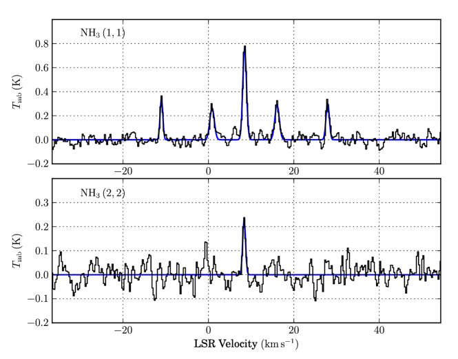
Figure 1: ${\rm NH_{3}}(J,K)=(1,1)$ (upper panel) and $(J,K)=(2,2)$ (lower panel) line profiles (black histogram) observed with the Nobeyama 45 m telescope toward the B335. Blue curves represent the best-fit results of Gaussian fitting (Section 3.1). The rms noise levels are $42\,{\rm mK}$ in $T_{\rm mb}$ for both spectra.

The spectrum of the ${\rm NH_{3}}(J,K)=(1,1)$ transition, which consists of five hyperfine groups, and the main component of the $(2,2)$ transition were obtained with good signal-to-noise ratios for the 45 m telescope. Figure 1 shows the spectra of the ${\rm NH_{3}}(J,K)=(1,1)$ and $(2,2)$ transitions obtained at the position of the IRAS source in B335. No emission in the $(3,3)$ transition was detected.

To estimate the optical depth and gas kinetic temperature, we analyzed the hyperfine structures that are caused by the electric quadrupole moment of the nitrogen nucleus. We derived the peak main-beam temperatures ($T_{\rm mb}$) and intrinsic velocity widths ($\Delta v$) by fitting each line component with a Gaussian function. We assumed that all hyperfine components have equal beam filling factors and excitation temperatures. We estimated the optical depth of the ${\rm NH_{3}}(1,1)$ main component [$\tau(1,1,m)$], the rotational temperature [$T_{\rm rot}(2,2;1,1)$] that describes the relative population between the $(1,1)$ and $(2,2)$ levels, and the kinetic temperature ($T_{\rm k}$) by following the analysis in a previous work by Mangum et al. (1992). With the parameters of the best-fit results (summarized in Table 3) shown by the blue curves in Figure 1, we obtained $\tau(1,1,m)=1.5\pm 0.9$, $T_{\rm rot}(2,2;1,1)=12.9\pm 1.1\,{\rm K}$, and $T_{\rm k}=15.1\pm 1.5\,{\rm K}$. The rotational temperature is almost equal to the kinetic temperature for the range of $T_{\rm rot}(2,2;1,1)\lesssim 20\,{\rm K}$ (Danby et al., 1988). Therefore, we determined that the B335 core has a mean kinetic temperature of $\sim{\rm 15\,K}$ over the beam area of the 45 m telescope ($\sim 80\arcsec$), and used this temperature to estimate the isothermal sound speed and the column density from the molecular line data.

3.2 87GHz Continuum Emission

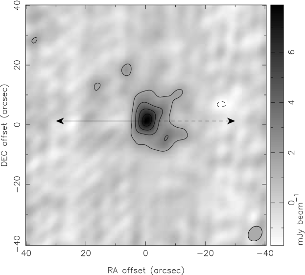
Figure 2: $87\,{\rm GHz}$ continuum image toward the IRAS source in B335 observed with the NMA. Contours start from the $3\sigma$ level with a $3\sigma$ interval, where $1\sigma=0.56\,{\rm mJy\,beam^{-1}}$. Dashed contours show the $-3\sigma$ level. Solid and dashed arrows in the image indicate the outflow directions of blue and red lobes, respectively. The ellipse at the bottom right corner indicates the synthesized beam size ($5\farcs 33\times 4\farcs 31$ with a position angle of $-37\fdg 2$).

We detected $87\,{\rm GHz}$ continuum emission with the NMA toward the IRAS source in B335, as shown in Figure 2. The peak position was measured to be ${\rm R.A.}=19^{\rm h}34^{\rm m}35\fs 2$, ${\rm decl.}=+07^{\circ}27^{\prime}23\farcs 8$ (B1950), which is consistent with the peak position of the $1.3\,{\rm mm}$ continuum images (Huard et al., 1999; Yen et al., 2010). The $87\,{\rm GHz}$ continuum image shows an elongated emission structure perpendicular to the outflow lying from east to west (Hirano et al., 1988). Furthermore, a cavity-like distribution in the red-lobe side of the molecular outflow can be seen which is quite similar to that in the $1.3\,{\rm mm}$ continuum image shown by Yen et al. (2010) and supports their suggestion that this distribution traces the wall of the outflow cavity. The beam deconvolved size, peak intensity, and total flux density (above the $3\sigma$ contour) are $9\farcs 2\times 6\farcs 4$ (corresponding to $1380\,{\rm AU}\times 960\,{\rm AU}$), $7.89\pm 0.56\,{\rm mJy\,beam^{-1}}$, and $33.1\pm 0.17\,{\rm mJy}$, respectively.

As mentioned in Chandler & Sargent (1993), contribution from free–free emission is considered to be negligible when taking into account the extrapolation from the flux at $3.6\,{\rm cm}$. Thus, we determine that the $87\,{\rm GHz}$ continuum emission comes from a dust envelope surrounding a protostellar object. Under the condition of being optically thin for thermal dust emission, the dust envelope mass ($M_{\rm env}$) was estimated using the equation $M_{\rm env}=S_{\nu}d^{2}/\kappa_{\nu}B_{\nu}(T_{\rm d})$, where $S_{\nu}$ is the total flux density, $\kappa_{\nu}$ is the dust mass opacity coefficient, $T_{\rm d}$ is the dust temperature, $d$ is the source distance, and $B_{\nu}$ is the Planck function. By combining our $87\,{\rm GHz}$ and image band $99\,{\rm GHz}$ measurements with the flux densities at millimeter wavelengths estimated by Keene et al. (1983), Chandler et al. (1990), and Hirano et al. (1992), we obtained a spectral index of $\alpha=3.3\pm 0.13$ for $S_{\nu}\propto\nu^{\alpha}$. The spectral index gives $\beta=1.3\pm 0.13$ for the emissivity law, $\kappa_{\nu}\propto\nu^{\beta}$, using the approximated relation, $\beta=\alpha-2$, which is valid for millimeter wavelengths (Beckwith et al., 2000). Thus, given $\kappa_{\rm 230\,GHz}=0.01\,{\rm cm^{2}\,g^{-1}}$ (André, 1994), we obtain a dust mass opacity of $\kappa_{\rm 87\,GHz}=2.8\times 10^{-3}\,{\rm cm^{2}\,g^{-1}}$. The dust envelope mass is estimated to be $M_{\rm env}\approx 0.19\,M_{\sun}$ with a dust temperature of $30\,{\rm K}$ (Chandler & Sargent, 1993).

3.3 ${\rm H^{13}CO^{+}}$ Line Emission

3.3.1 Integrated Intensity and Channel Maps

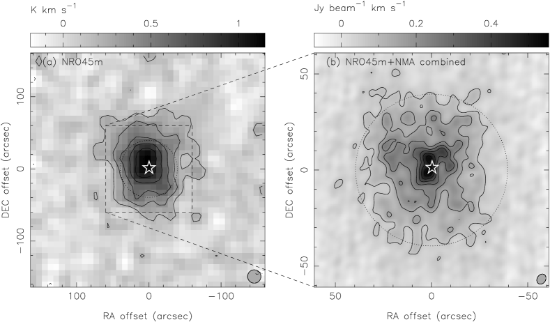
Figure 3: Total integrated intensity maps of B335 in the ${\rm H^{13}CO^{+}}(J=1$–$0)$ line emission obtained with the 45 m telescope (left) and by combining the 45 m telescope and NMA data (right). Contour intervals are $3\sigma$, starting from the $3\sigma$ levels of the images where $1\sigma$ noise levels are $62\,{\rm mK\,km\,s^{-1}}$ in $T_{\rm mb}$ for the 45 m telescope map and $24\,{\rm mJy\,beam^{-1}\,km\,s^{-1}}$ for the combined map. Dashed contours show the $-3\sigma$ level. The open star in each map is the peak position of the $87\,{\rm GHz}$ continuum emission observed with the NMA. The beam size for each map is shown as a filled circle or filled ellipse at the bottom right corner. Dotted circle in the combined image indicates the field of view, i.e., FWHM primary beam size of the NMA observations.

The panels of Figure 3 show the integrated intensity images of the ${\rm H^{13}CO^{+}}(J=1$–$0)$ line emission over the LSR velocity range from $8.08$ to $8.95\,{\rm km\,s^{-1}}$ made using the 45 m telescope data (left) and the combined 45 m telescope and NMA data (right). We should note that this combined map includes the effect of the primary beam attenuation of the NMA so that extended emission toward the outside of the image seen in the 45 m telescope image is not reproduced in the combined image.

The ${\rm H^{13}CO^{+}}$ emission in the 45 m telescope map has a single-peaked spatial distribution and shows an elongation from north to south. The size of the ${\rm H^{13}CO^{+}}$ core above the $3\sigma$ level is $\sim 0.10\,{\rm pc}\times 0.09\,{\rm pc}$, with a P.A. of $\sim 0^{\circ}$. The 45 m telescope plus NMA combined map shown in the right panel of Figure 3 clearly depicts the detailed structure of the inner core including large-scale flux distributions with a high resolution. The higher contours of $\gtrsim 12\sigma$ show an elongated distribution from north to south with a size of $\sim 3000\,{\rm AU}\times 1500\,{\rm AU}$, which is believed to be an inner dense envelope associated with a central stellar source. The envelope has a double peak near the center, and the $87\,{\rm GHz}$ continuum source is located between the peaks. The elongation of the core and inner envelope is perpendicular to the molecular outflow axis (e.g., Hirano et al., 1988). In the 45 m telescope map, there are faint ridges from the center along the P.A. of $\sim 70^{\circ}$, $\sim-45^{\circ}$, and $\sim-135^{\circ}$, and they can be seen more clearly in the combined map. Taking the outflow direction and opening angle into account ($\sim 45^{\circ}$; Hirano et al., 1988), we believe that these ridges are related to the outflow activity.

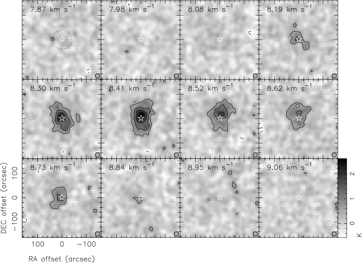
Figure 4: Velocity channel maps of B335 in the ${\rm H^{13}CO^{+}}(J=1$–$0)$ line emission taken with the 45 m telescope. The central LSR velocity in ${\rm km\,s^{-1}}$ for each channel is shown in the upper left corner. Contour intervals are the same as in Figure 3, and the $1\sigma$ noise level is $0.19\,{\rm K}$ in $T_{\rm mb}$. The open star, filled circle in each panel, and dotted circle are the same as in Figure 3.

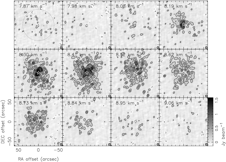
Figure 5: Velocity channel maps (CLEANed synthesized images) of B335 in the ${\rm H^{13}CO^{+}}(J=1$–$0)$ line emission obtained by combining the 45 m telescope and NMA data. The central LSR velocity in ${\rm km\,s^{-1}}$ for each channel is shown in the upper left corner. Contour intervals are the same as in Figure 3 and $1\sigma$ noise level is $45\,{\rm mJy\,beam^{-1}}$. The open star, filled ellipse in each panel, and dotted circle are the same as in Figure 3.

In the velocity channel maps obtained with the 45 m telescope shown in Figure 4, the emission peaks are located at the north of the $87\,{\rm GHz}$ continuum source in the velocity range $V_{\rm LSR}=8.19$–$8.62\,{\rm km\,s^{-1}}$, and at the south in the velocity range $V_{\rm LSR}=8.73$–$8.84\,{\rm km\,s^{-1}}$. This velocity gradient is perpendicular to the outflow axis and can be interpreted as the rotational motion of the B335 core. On the other hand, in the channel maps of combined data shown in Figure 5, it is difficult to identify the corresponding velocity gradient because of the complicated emission distribution. More detailed kinematics of the B335 core are discussed in Section 3.3.3 and 4.2 using position–velocity (PV) diagrams made from the 45 m telescope and combined images.

3.3.2 Mass and Column Density Profile in the Core

In order to estimate the column density of the B335 protostellar core, we analyzed the ${\rm H^{13}CO^{+}}$ images made from the 45-m telescope and the combined NMA plus 45 m telescope data.

Under the local thermodynamic equilibrium (LTE) assumption, the ${\rm H_{2}}$ column density can be calculated using the following formula:

$$N_{\rm H_{2}} \simeq 5.58\times 10^{10}\frac{1}{X({\rm H^{13}CO^{+}})}$$ (1)

$$\times\frac{T_{\rm ex}+0.69}{e^{-4.16/T_{\rm ex}}}\frac{\tau}{1-e^{-\tau}}\left(\frac{\int T_{\rm mb}dv}{\rm K\,km\,s^{-1}}\right)\quad{\rm cm^{-2}},$$

where $T_{\rm ex}$ is the excitation temperature, $\tau$ is the optical depth of the ${\rm H^{13}CO^{+}}$ line, and $X({\rm H^{13}CO^{+}})$ is the fractional abundance of ${\rm H^{13}CO^{+}}$. When deriving of Equation (1), we used the permanent dipole moment $\mu=4.07\,{\rm Debye}$ (Haese & Woods, 1979) and the rotational constant $B=43377.17\,{\rm MHz}$. To obtain a complementary expression for the combined synthesized image, we convert the antenna temperature into the flux density $S_{\nu}$ in the ${\rm Jy\,beam^{-1}}$ through $S_{\nu}=\left(2k_{\rm B}/\lambda^{2}\right)\Omega_{\rm b}T_{\rm mb}$, where $\Omega_{\rm b}$ is the beam solid angle given by $\pi\theta_{\rm maj}\theta_{\rm min}/4\ln 2$. Thus, we have

$$N_{\rm H_{2}} \simeq 9.01\times 10^{12}\frac{1}{X({\rm H^{13}CO^{+}})}\frac{T_{\rm ex}+0.69}{e^{-4.16/T_{\rm ex}}}\frac{\tau}{1-e^{-\tau}}$$ (2)

$$\quad\times\left(\frac{\theta_{\rm maj}\theta_{\rm min}}{\rm arcsec^{2}}\right)^{-1}\left(\frac{\int S_{\nu}dv}{\rm Jy\,km\,s^{-1}}\right)\quad{\rm cm^{-2}}.$$

We assumed the excitation temperature of ${\rm 15\,K}$ from the ${\rm NH_{3}}$ analysis (Section 3.1) and the ${\rm H^{13}CO^{+}}$ line of the optically thin limit. We assumed $X({\rm H^{13}CO^{+}})$ to be $8.3\times 10^{-11}$ (Frerking et al., 1987). The derived total mass from the 45 m telescope map (the left panel of Figure 3) is $\approx 1.2\,M_{\sun}$.

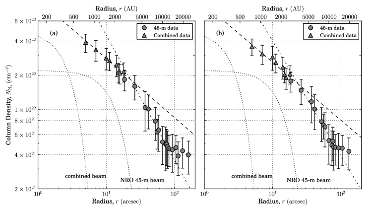
Figure 6: Radial profile of ${\rm H_{2}}$ column density in the B335 core made from the ${\rm H^{13}CO^{+}}(J=1$–$0)$ image obtained with the 45 m telescope only (filled circles) and the combined 45 m telescope and NMA data (filled triangles). Panel (a) shows the profile without the mask in the cavity regions and panel (b) shows that with the mask. Dot-dashed and dashed lines in the plot indicate the best-fit results of power-law fitting with the fitting range of $750$–$4000\,{\rm AU}$ and $4000$–$15{,}000\,{\rm AU}$, respectively. Dotted curves indicate approximated beam patterns of 45 m telescope image and the combined image, Gaussian functions with the FWHM of $25\farcs 0$ and $5\farcs 0$, respectively.

We derived the radial column density profile in the B335 core from the column density map calculated by the above formula. The column densities were calculated from re-gridded images with cell sizes corresponding to the spatial resolutions of the images, i.e., $5^{\prime\prime}$ ($750\,{\rm AU}$) for the combined image and $25^{\prime\prime}$ ($3750\,{\rm AU}$) for the 45 m image. The column density profile was made as a function of the radius from the $87\,{\rm GHz}$ peak using the distributions of the estimated column densities over the re-gridded cells. In order to calculate the column density, the 45 m plus NMA image needed to be corrected for the primary beam attenuation, which increases the noise level in the outer region of the image. Hence, the column density profile in the outer region of the core was derived using the 45 m telescope data, and the 45 m plus NMA combined data were used to fill in the inner region of $\lesssim 3000\,{\rm AU}$ where the data cannot be obtained from 45m telescope data. Figure 6 represents the resulting ${\rm H_{2}}$ column density profiles obtained in the above procedure. As suggested in Section 3.3.1, the B335 core could be affected by the outflow. To examine this effect we also made the column density profile by masking out the regions with P.A. of $67\fdg 5$–$112\fdg 5$ and $247\fdg 5$–$292\fdg 5$. The masking angle of $45^{\circ}$ was chosen to match the opening angle of the outflow: $\sim 45^{\circ}$ by Hirano et al. (1988) and $\sim 41^{\circ}$ by Harvey et al. (2001). Figure 6(a) and (b) show the ${\rm H_{2}}$ column density profile without and with the masking, respectively. For both profiles, we can see that the column densities estimated from the 45 m and combined data are smoothly connected around the radius of $\sim 3000\,{\rm AU}$, and that the profiles in the inner radius are shallower than those in the outer radius.

The column density profiles were fitted by two power-law functions of $N(r)=N_{0}(r/r_{0})^{-s}$, where $s$ is the power-law index and $N_{0}$ is the column density at $r=r_{0}=1500\,{\rm AU}$. Since Figure 6 clearly shows two different slopes between the inner and outer regions, we estimated the turnover radius at which the power-law index changes. We evaluated the correlation coefficient of the power-law fitting in the range of $r_{\rm fit,i}$–$r_{\rm fit,o}$, where the inner radius ($r_{\rm fit,i}$) was variable and the outer radius ($r_{\rm fit,o}$) was fixed to $r_{\rm fit,o}=15{,}000\,{\rm AU}$. As a result, we found that the correlation coefficient of the fitting decreased exceedingly when the fitting inner radius was taken inside of $4000\,{\rm AU}$. Thus, we adopted a turnover radius of $4000\,{\rm AU}$ in this paper and performed the power-law fittings in the two regions of $750$–$4000\,{\rm AU}$ and $4000$–$15{,}000\,{\rm AU}$ separately.

For the inner region ranging from $750$ to $4000\,{\rm AU}$, we obtained $N_{\rm H_{2}}(r)=(2.8\pm 1.0)\times 10^{22}(r/1500\,{\rm AU})^{-(0.52\pm 0.06)}~{}{\rm cm^{-2}}$ without masking, and $N_{\rm H_{2}}(r)=(2.6\pm 1.0)\times 10^{22}(r/1500\,{\rm AU})^{-(0.51\pm 0.05)}~{}{\rm cm^{-2}}$ with masking. For the outer region from $4000$ to $15{,}000\,{\rm AU}$, we obtained $N_{\rm H_{2}}(r)=(4.5\pm 1.3)\times 10^{22}(r/1500\,{\rm AU})^{-(1.10\pm 0.16)}~{}{\rm cm^{-2}}$ without masking and $N_{\rm H_{2}}(r)=(4.0\pm 1.3)\times 10^{22}(r/1500\,{\rm AU})^{-(1.01\pm 0.16)}~{}{\rm cm^{-2}}$ with masking. The column density profile obtained with masking was estimated to be slightly shallower than that without the masks. From our fitting result, the column density at $r=6000\,{\rm AU}$ is $\approx 9.7\times 10^{21}\,{\rm cm^{-2}}$, which is consistent with the estimate by Saito et al. (1999), $N_{\rm H_{2}}(6000\,{\rm AU})\sim 6.3\times 10^{21}\,{\rm cm^{-2}}$. Using our results, we examined the density distribution of the B335 core (discussed in Section 4.1.1) and estimated the total mass of gas associated with the B335 core to be $\approx 0.78M_{\sun}$ within the radius of $6000\,{\rm AU}$.

3.3.3 Position–Velocity Diagrams

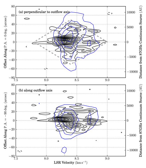
Figure 7: Position-velocity diagrams of the ${\rm H^{13}CO^{+}}(J=1$–$0)$ line emission for the B335 core made from the 45 m telescope image data (blue contours) and the combined data (gray scale with black contours). Panel (a) and (b), respectively, show the diagrams along ${\rm P.A.}=0^{\circ}$ (perpendicular to the outflow axis) and ${\rm P.A.}=90^{\circ}$ (along the outflow axis), passing through the $87\,{\rm GHz}$ continuum source.

To examine the overall velocity structure in the B335 core, we made PV diagrams using the combined ${\rm H^{13}CO^{+}}(J=1$–$0)$ line data as shown in Figure 7, with black contours and gray scales. We chose the two axes of ${\rm P.A.}=0^{\circ}$ (perpendicular to the outflow axis) and ${\rm P.A.}=-90^{\circ}$ (along the outflow axis), passing through the $87\,{\rm GHz}$ continuum source. The comparison with the diagrams made from the low-spatial-resolution 45 m data overlaid with blue contours demonstrates a drastic effect of data combining. Along the P.A. of $0^{\circ}$, the 45 m telescope data show a slight velocity gradient, $\sim 1.0\,{\rm km\,s^{-1}\,pc^{-1}}$ over a scale of $20{,}000\,{\rm AU}$. This gradient is comparable to the typical value of the cores in the Taurus dark cloud (Goodman et al., 1993). If the gradient represents a solid-body-like rotation of the core, then it is converted into an angular velocity of $\omega\sim 3.2\times 10^{-14}\,{\rm rad\,s^{-1}}$. On the other hand, the diagram of P.A. of $-90^{\circ}$ does not show a conspicuous velocity gradient.

The diagrams of the 45 m and NMA combined data show line broadening and a double-peaked intensity profile at the core center (offset $=0\arcsec$). With a broadening line width toward the core center, the diagram along the P.A. of $0^{\circ}$ shows an overall symmetrical diamond-like structure (represented by a dashed line in light gray). We calculated intensity-weighted first and second moments defined by $M_{1}=\int I(v)vdv/\int I(v)dv$ and $M_{2}=\sqrt{\int I(v)(v-M_{1})^{2}dv/\int I(v)dv}$, respectively. The second moment at the center (offset of $0\arcsec$) was $M_{2}\approx 0.25\,{\rm km\,s^{-1}}$, whereas that at the offset of $20\arcsec$ was $0.17\,{\rm km\,s^{-1}}$. The double-peaked profile at the core center is also slightly visible in the diagram made from the 45-m telescope data. This profile has asymmetrical features that are more enhanced in the blueshifted peak than in the redshifted one. This blue-skewed profile is maybe due to the infall motion of the core (Zhou et al., 1993, 1994) because the ${\rm H^{13}CO^{+}}(J=1-0)$ line emission is moderately optically thick around the systemic velocity (see Section 4.1.3).

The center of the overall symmetrical emission distribution (lowest contour), as represented with a dashed diamond in Figure 7(a), is approximately $\sim 8.4\,{\rm km\,s^{-1}}$ and $0\arcsec$, which is considered to be the dynamical center of the B335 core. Since the LSR velocity of $8.4\,{\rm km\,s^{-1}}$ is consistent with the peak velocities of the ${\rm NH_{3}}$ main components (Section 3.1), we adopt an LSR velocity of $8.4\,{\rm km\,s^{-1}}$ as the systemic velocity of the protostellar system.

4 DISCUSSION

4.1 Density Structure of the Core

4.1.1 Overall Structure of the Core

When a molecular cloud core has a density distribution of $\rho(r)\propto r^{-p}$, the profile of the column density integrated along the line of sight has a relation of $N(r)\propto r^{-s}\propto r^{1-p}$. Hence, our obtained indices of $s\approx 0.5$ in the inner part of the B335 core and of $s\approx 1$ in the outer part correspond to $p\approx 1.5$ and $p\approx 2$, respectively. We note that these indices barely varied even if we considered the influence of the cavity in the core made by the outflow.

The column density profile derived from our 45 m and combined data with masking (Section 3.3.2) can be converted into the number density distribution:

$$n(r)\approx 1.2\times 10^{5}~{}{\rm cm^{-3}}$$

$$\left\{\begin{array}[]{ll}\left(\frac{r}{\rm 4000\,AU}\right)^{-1.51}\quad{\rm for~{}}750\,{\rm AU}\leqslant r\leqslant 4000\,{\rm AU},\\ \left(\frac{r}{\rm 4000\,AU}\right)^{-2.01}\quad{\rm for~{}}4000\,{\rm AU}\leqslant r\leqslant 15{,}000\,{\rm AU}.\end{array}\right.$$ (5)

Most previous studies have derived density profiles for the B335 star-forming core similar to our observational results: inner and outer indices of $-1.51$ and $-2.01$, respectively, with a turnover radius of $\sim 4000\,{\rm AU}$. A power-law index of $p\sim 1.95$ for the density profile was estimated from single-dish observations of the ${\rm C^{18}O}(J=1$–$0)$ and ${\rm H^{13}CO^{+}}(J=1$–$0)$ line emissions (radius range of $4200$–$25{,}000\,{\rm AU}$) by Saito et al. (1999). From near-infrared extinction measurements, Harvey et al. (2001) suggested that the B335 core has a constant power-law index of $p=1.91$ over the region $2000$–$15{,}000\,{\rm AU}$, and otherwise displays inside-out collapse with an infalling radius (see Section 4.2) of $\sim 26\arcsec$ (corresponding to $\sim 3900\,{\rm AU}$). Harvey et al. (2003a, b) also suggested a single power law with $p=1.55$ within the inner $\lesssim 3000\,{\rm AU}$ region from interferometric observations of $1.2$ and $3.0\,{\rm mm}$ continuum. These results agree well with our estimate of the density profile from the ${\rm H^{13}CO^{+}}(J=1$–$0)$ data. Meanwhile, detailed analysis of SCUBA $450$ and $850\,{\rm\micron}$ continuum maps by Shirley et al. (2002) showed that the model with a power-law index of $p=1.8$ well describes the data as a best-fit result, and suggested an infalling radius of $1000\,{\rm AU}$, which is smaller than estimates in our as well as previous studies. Doty et al. (2010) recently conducted an unbiased fitting to the dust continuum observations toward B335. For the power-law density distribution, they obtained $p=1.5$–$1.9$ throughout the envelope, although they did not find strong evidence of inside-out collapse with an infalling radius of $\sim 1000\,{\rm AU}$.

4.1.2 Inner Structure of the Core

We confirmed the above estimate of the density profile from our combined ${\rm H^{13}CO^{+}}(J=1$–$0)$ line data using an analysis of the visibility data of the $87\,{\rm GHz}$ continuum emission observed with the NMA. This approach of directly examining in the $u$–$v$ domain enables us to avoid possible artifacts caused by the deconvolution of interferometric images.

When discussing the emission distribution of the inner region of an envelope observed with interferometers, we should consider the temperature distribution of the envelope. We consider the observed intensity as a function of the impact parameter, $I_{\nu}(r_{\rm b})$, from an optically thin dust envelope that has a spherical density distribution, $\rho(r)$, and a dust temperature, $T_{\rm d}(r)$. If the density and temperature follow radial power laws, $\rho\propto r^{-p}$ and $T_{\rm d}\propto r^{-q}$, and if we assume that the opacity does not vary along the line of sight, then the intensity profile also has a power-law profile, $I_{\nu}(r_{\rm b})\propto r_{\rm b}^{-(p+q-1)}$, in the Rayleigh–Jeans regime. We assumed that the extent of source intensity $I_{\nu}(r_{\rm b})$ is sufficiently compact in the primary beam. The visibility amplitude as a function of $u$–$v$ distance ($b$) can be given by $V(b)\propto b^{p+q-3}$ for $3/2<p+q<3$ (see the Appendix for details).

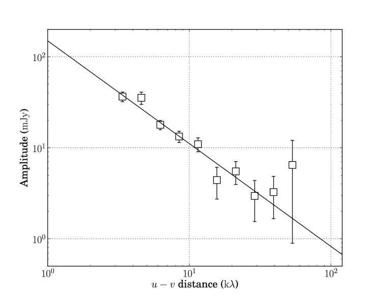
Figure 8: Binned visibility amplitude of the $87\,{\rm GHz}$ continuum data taken with the NMA as a function of $u$–$v$ distance. Binning is logarithmic and amplitudes are obtained as vectorial average of the complex visibilities in each bin. A solid line shows the best-fit power-law function.

Figure 8 shows a plot of binned visibility amplitudes as a function of the $u$–$v$ distance for the $87\,{\rm GHz}$ continuum data. The binning is logarithmic, and the amplitudes are obtained as the vectorial average of the complex visibilities in each bin. The decrease in visibility amplitude with $u$–$v$ distance can be interpreted as a power law. We fitted the visibility amplitude profile with a power-law function of the form $A\times b^{-\xi}$. The best-fit power-law index is $\xi=1.13\pm 0.06$ (solid line in the plot), which can be converted into a power-law index with an intensity distribution of $p+q-1=0.87$. The power-law index of dust temperature distribution is expected to depend on the opacity, $T_{\rm d}(r)\propto L^{q/2}r^{-q}$, where $q=2/(4+\beta)$ (Doty & Leung, 1994). Thus, the power-law index of the density distribution is estimated to be $p=1.49$ for $\beta=1.3$ (see Section 3.2), which shows a good agreement with the estimate from the combined ${\rm H^{13}CO^{+}}$ data (Section 4.1.1).

4.1.3 Uncertainties of Density Profile

There are several uncertainties included in the derived density distribution. In this section, we examine the effect of opacity, assumption of uniform temperature, index conversion from column density to volume density profiles, and ${\rm H^{13}CO^{+}}$ fractional abundance.

First, we investigate the effect of the optical depth of ${\rm H^{13}CO^{+}}$ line emission, because the decrement of derived column densities in the inner radii might be due to larger optical depth within the $5\arcsec$ beam. Saito et al. (1999) indicated that the ${\rm H^{13}CO^{+}}$ emission is optically thin even at the center of an $18\arcsec$ beam from the measured ${\rm HC^{18}O^{+}}$ to ${\rm H^{13}CO^{+}}$ peak intensity ratio of $\sim 5.8$ and expected abundance ratio, $X({\rm H^{13}CO^{+}})/X({\rm HC^{18}O^{+}})$, of $5.5$. Furthermore, the integrated intensity ratio of ${\rm HC^{18}O^{+}}$ to ${\rm H^{13}CO^{+}}$ implies that ${\rm H^{13}CO^{+}}$ emission should be optically thin at the center. According to Figure 1 in Saito et al. (1999), the line ratio actually ranges from $\sim 2.8$ to $\sim 5.8$ across the velocity; the lowest line ratio indicates that ${\rm H^{13}CO^{+}}$ emission is marginally thick, $\tau\sim 2$ at maximum in certain velocities. This opacity enhancement is limited only to a narrow velocity range, so it does not introduce a significant error when estimating the column density near the center, i.e., the underestimate. Therefore, the effect of the optical depth cannot account for the turnover around the radius of $4000\,{\rm AU}$.

Second, we assumed that the core has a uniform temperature distribution that does not have much effect on the estimate of the column density. If we adopt the temperature profile from Evans et al. (2005), for example, then the difference in temperature between radii of $750\,{\rm AU}$ and $20{,}000\,{\rm AU}$ should be a factor of $\sim 2$. From Equation (2), the uncertainty of the column density estimate expected by this temperature variation could be derived as $\pm\sim 10\%$ at most.

Third, the derivation of the density profile of the core from the column density distribution depends on the radial finiteness of the core traced by the ${\rm H^{13}CO^{+}}$ molecular line emission. For a spherical core with a size of $R_{\rm out}$ and a power-law density profile of $\rho(r)=\rho_{0}(r/r_{0})^{-p}$, the column density that is given by integrating the densities along the line of sight at the impact parameter $r_{\rm b}$ can be expressed as

$$N(r_{\rm b})=\int^{\arccos(r_{\rm b}/R_{\rm out})}_{-\arccos(r_{\rm b}/R_{\rm out})}\rho(r)d\theta=N_{0}\left(\frac{r_{\rm b}}{r_{0}}\right)^{-p+1},$$ (6)

where

$$N_{0}=\rho_{0}r_{0}\int^{\arccos(r_{\rm b}/R_{\rm out})}_{-\arccos(r_{\rm b}/R_{\rm out})}\cos^{p}\theta d\theta,$$ (7)

and the variable $\theta$ is an angle between a radial vector $r$ and the plane of the sky. Therefore, the coefficient of $N_{0}$ is also a function of $r_{\rm b}$ so that the column density profile deviates from a power-law of the form $N(r_{\rm b})\propto r_{\rm b}^{-p+1}$. Moreover, if the core has different power-law dependencies between the inner and outer regions, then the simple prediction of the column density profile in Equation (6) is not exactly valid. Figure 9 shows the column density profiles of cores that have power-law density distributions with a cutoff radius $R_{\rm out}$. The dashed lines indicate the profiles for the predictions of $\propto r^{-p+1}$. For the case of a single power-law density distribution of $\rho(r)\propto r^{-2}$ as shown in Figure 9(a), the resulting column density coincides well with the dependency of $\propto r^{-1}$ at radii smaller than $\sim 0.1R_{\rm out}$. However, it tends to depart from the power-law dependency and become steeper with increasing radius. Figure 9(b) shows the column density profile for the core with density distributions of $\rho(r)\propto r^{-1.5}$ for $r\leqslant 0.125R_{\rm out}$ and $\rho(r)\propto r^{-2}$ for $r>0.125R_{\rm out}$. This plot demonstrates that the column density profile of a core that has inner and outer regions with different power-law density distributions can be estimated to be steeper than the simple prediction of $N(r_{\rm b})\propto r_{\rm b}^{-p+1}$. We examined the uncertainties caused by these effects when converting the column density profile into the density profile, and we found that the true density profile is likely to be shallower by $\sim 0.1$ at most in the power-law index than for our estimates.

Finally, as for the abundance of ${\rm H^{13}CO^{+}}$, recent studies of chemical evolution in star-forming cores have shown that the abundance of ${\rm HCO^{+}}$, which is a daughter species of ${\rm CO}$, decreases at radii that are smaller than the ${\rm CO}$ sublimation radius (Lee et al., 2004; Aikawa et al., 2008). Nevertheless, it is shown that the abundance of ${\rm HCO^{+}}$ at the inner radii increases with the evolution of core collapse after a central stellar object is born. Evans et al. (2005) simulated a large number of molecular line profiles from B335 using various physical models. By the use of a self-consistent chemical model with core evolution, the result showed that the abundance of ${\rm HCO^{+}}$ hardly changes along the core radius. The shallower profile at smaller radii can be affected by the radial distribution of the ${\rm H^{13}CO^{+}}$ abundance, although it is not expected to be dominant.

The possible effects of radial dependence in the ${\rm H^{13}CO^{+}}$ abundance and the finite core radius oppose one another. It is difficult to estimate how they contribute to our data. Nevertheless, by taking into account the agreement of the column density profiles in the inner region of the B335 core between the derivations from the combined ${\rm H^{13}CO^{+}}$ and dust continuum data, we determine that the effects of variation in optical depth and radius dependence in the ${\rm H^{13}CO^{+}}$ abundance are likely to be negligible. Moreover, the agreement between the profile indices derived from our data with those from the extinction analysis of near-infrared data indicates that the effect of these uncertainties, especially in the temperature and fractional abundance of ${\rm H^{13}CO^{+}}$, is not very considerable. In other words, our ${\rm H^{13}CO^{+}}$ data well represent the column density structure of the core, which mostly ensures the validity of our analysis for the physics of star formation.

4.2 Velocity Structure of the Core

We performed model calculations of the PV diagrams and investigated which model reproduces the observed signatures of the PV diagram in the ${\rm H^{13}CO^{+}}$ line well. For comparison with the observed results, the model calculations were performed with different radial distributions of the infalling velocities and also for three different assumed central stellar masses.

4.2.1 Model Calculations of PV Diagram

We assume a contracting spherical star-forming core with rotation as described in detail below. Most of the parameters for the calculations simulating PV diagrams were taken from our observational results and previous studies.

The core has a size of $20{,}000\,{\rm AU}$ and the radial density profile in Equation (5) shows power-law dependencies ($\rho\propto r^{-p}$) of $p=1.5$ in the inner ($r<4000\,{\rm AU}$) and $p=2$ in the outer ($r\geqslant 4000\,{\rm AU}$) regions. Such a difference in power-law indices is naturally expected from the isothermal collapse model because of the boundary of the inner free-falling region and the outer region in which the condition at the stage of the formation of a central stellar object is expected to be conserved. The boundary radius is referred to as the infalling radius ($r_{\rm inf}$), and therefore our derived density profile indicates $r_{\rm inf}=4000\,{\rm AU}$.

We also introduced the rotational motion of the core. The inclination angle of the rotation axis from the plane of the sky should be considered because it affects the line-of-sight velocity of rotational motion. We assumed that the rotation axis corresponds to the outflow axis whose inclination angle for B335 was estimated to be $10^{\circ}$ (Hirano et al., 1988), $8\pm 5^{\circ}$ (Cabrit et al., 1988), and $9\pm 1^{\circ}$ (Moriarty-Schieven & Snell, 1989). We adopted an inclination angle of $10^{\circ}$ for the rotation axis in our calculations. In the free-fall region with $r\leqslant r_{\rm inf}$, we adopted the increasing rotational velocity which is inversely proportional to the radius owing to the angular momentum conservation during collapse. Such a velocity field in infalling envelopes was indeed suggested observationally (e.g., L1551-IRS5 by Momose et al., 1998). The overall velocity gradient from the 45 m telescope observations, $1.0\,{\rm km\,s^{-1}\,pc^{-1}}$ ($\omega=3.2\times 10^{-14}\,{\rm rad\,s^{-1}}$), can be regarded as the initial angular momentum of the core, which is still preserved in the outer radius of $r\geqslant r_{\rm inf}=4000\,{\rm AU}$. For the thermal line broadening, we set the line-of-sight velocity width of $0.15\,{\rm km\,s^{-1}}$ for ${\rm H^{13}CO^{+}}$ molecules at $T_{\rm k}=15\,{\rm K}$.

We calculated radiative transfer equations to estimate the relative intensity distributions and verify the effect of optical depth. Assuming a two-level state, the populations in rotational levels of an ${\rm H^{13}CO^{+}}$ molecule were calculated using the Einstein $A$ coefficient and the collisional rate coefficients with ${\rm H_{2}}$ from Gerin et al. (2009) and Flower (1999). The final model PV diagrams were smoothed with Gaussian functions whose FWHMs are the same as actual resolutions of the combined image for both the spatial and velocity directions.

4.2.2 Comparison of Model Calculations of PV Diagrams with Observations

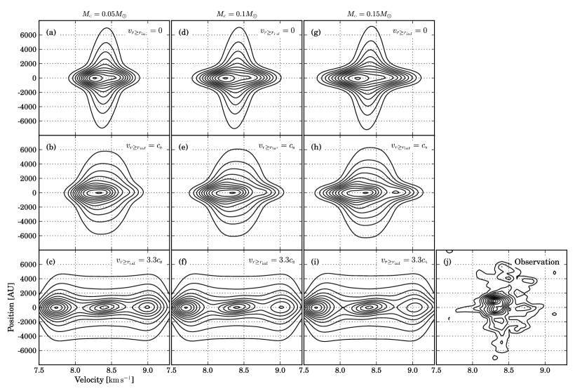
Figure 10: Panels (a)–(i) show simulated PV diagrams by the simple calculations using models of contracting core with rotational motion. The cutting axis is perpendicular to the rotation axis. Panels (a), (b), and (c) show the model PV diagrams with $v_{r\geqslant r_{\rm inf}}=0\,{\rm km\,s^{-1}}$, $c_{\rm s}$, and $3.3\,c_{\rm s}$ with the central stellar mass of $M_{\rm c}=0.05M_{\sun}$, respectively. Panels (d)–(f) show the diagrams in the cases of $M_{\rm c}=0.1M_{\sun}$ and panels (g)–(i) show the cases of $M_{\rm c}=0.15M_{\sun}$. PV diagram of the ${\rm H^{13}CO^{+}}(J=1$–$0)$ line emission from B335 perpendicular to the outflow axis is shown in panel (j) with black contours. Contour intervals of model PV diagrams relative to the peaks are the same as those for the observed diagram.

We conducted simulations by varying the parameters of the inward velocity in the outer region ($r\geqslant r_{\rm inf}$) of the core, $v_{r\geqslant r_{\rm inf}}$, and the mass of the central stellar object to compare with observational results. We adopted the inward velocities in the outer region of $v_{r\geqslant r_{\rm inf}}=0\,{\rm km\,s^{-1}}$, $c_{\rm s}$, and $3.3\,c_{\rm s}$. The central stellar mass ($M_{\rm c}$) for B335 was estimated in a wide range in previous studies, e.g., Choi et al. (1995) estimated it to be $0.37\,M_{\sun}$ while $0.04M_{\sun}$ was suggested by Yen et al. (2010). In our model calculations, we used three values of the central stellar mass: $M_{\rm c}=0.05M_{\sun}$, $0.1M_{\sun}$, and $0.15M_{\sun}$. Figure 10 shows the calculated PV diagrams perpendicular to the rotation axis passing through the core center.

As for the inward velocities in the outer region of the core, the calculated PV diagrams for $v_{r\geqslant r_{\rm inf}}=0\,{\rm km\,s^{-1}}$ well reproduce the features in the observed PV diagram. The inward velocity in the outer region affects the overall line width in the PV diagram. Although the PV diagrams calculated with $v_{r\geqslant r_{\rm inf}}=c_{\rm s}$ are also similar to the observed result, the overall velocity widths seem to be larger than that of the observed one. The simulated diagrams with $v_{r\geqslant r_{\rm inf}}=3.3\,c_{\rm s}$ undoubtedly disagree with the observation. We found that the central stellar mass mainly contributes line broadening at the core center, which means that the infalling motion is more dominant than the spin-up rotation owing to the conservation of angular momentum around the core center. For the diagrams with $v_{r\geqslant r_{\rm inf}}=0\,{\rm km\,s^{-1}}$, it seems that line wings at the center position are not enough in the case of $M_{\rm c}=0.05M_{\sun}$ while they are excessive in the case of $M_{\rm c}=0.15M_{\sun}$. Consequently, we determine in our model calculations that the PV diagram with $v_{r\geqslant r_{\rm inf}}=0\,{\rm km\,s^{-1}}$ and $M_{\rm c}=0.1M_{\sun}$ well represents the observed PV diagram.

The calculated model PV diagram with $v_{r\geqslant r_{\rm inf}}=0\,{\rm km\,s^{-1}}$ and $M_{\rm c}=0.1M_{\sun}$ shows that the peak is skewed toward the blueshifted velocity and has a shoulder in the profile around the systemic velocity at the center position. These features in the model diagram are due to the ${\rm H^{13}CO^{+}}$ optical depth and are similar to the observational result. Hence, the suggestion discussed in Section 4.1.3 that the ${\rm H^{13}CO^{+}}(J=1$–$0)$ line is marginally optically thick is probably reasonable.

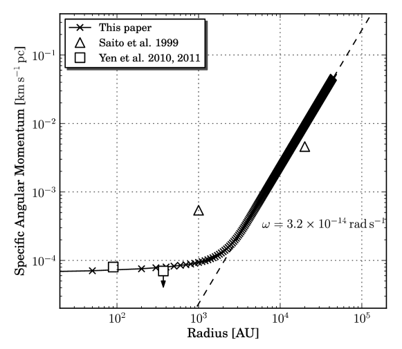
Figure 11: Radial distribution of specific angular momentum in our model calculation (Section 4.2) for the case of $v_{r\geqslant r_{\rm inf}}=0\,{\rm km\,s^{-1}}$ and $M_{\rm c}=0.1M_{\sun}$ (cross marks with solid line) as a function of radius. Open squares represent specific angular momenta measured from velocity gradients seen in the ${\rm C^{18}O}(J=2$–$1)$ and ${\rm CS}(J=7$–$6)$ envelopes by Yen et al. (2010, 2011), and open triangles denote specific angular momenta measured from ${\rm C^{18}O}(J=1$–$0)$ core and ${\rm H^{13}CO^{+}}(J=1$–$0)$ envelope by Saito et al. (1999). A dashed line indicates the profile of specific angular momentum of $\omega=3.2\times 10^{-14}\,{\rm rad\,s^{-1}}$.

In addition, we can obtain the radial distribution of the specific angular momentum from the profile of rotation velocity in the model calculations of PV diagrams. Figure 11 shows the radial distribution of specific angular momentum in the model that well represents the observation: the case of $v_{r\geqslant r_{\rm inf}}=0\,{\rm km\,s^{-1}}$ and $M_{\rm c}=0.1M_{\sun}$. We can see the spin-up rotation within the infall radius of $r_{\rm inf}=4000\,{\rm AU}$ as deviations from the solid-body rotation with an angular velocity of $\omega=3.2\times 10^{-14}\,{\rm rad\,s^{-1}}$. In previous observational studies, the specific angular momenta of the core and envelope in B335 have been measured at several radii from velocity gradients across the outflow axis. Yen et al. (2010, 2011) derived the specific angular momenta of $\lesssim 7\times 10^{-5}\,{\rm km\,s^{-1}\,pc}$ at a radius of $370\,{\rm AU}$ and $8\times 10^{-5}\,{\rm km\,s^{-1}\,pc}$ at $90\,{\rm AU}$ from velocity gradients seen in the ${\rm C^{18}O}(J=2$–$1)$ and ${\rm CS}(J=7$–$6)$ envelopes, respectively. They discussed the evolution of specific angular momentum, including the measurements by Saito et al. (1999) of $\sim 5.4\times 10^{-4}\,{\rm km\,s^{-1}\,pc}$ at $1000\,{\rm AU}$ and $\sim 4.6\times 10^{-3}\,{\rm km\,s^{-1}\,pc}$ at $20{,}000\,{\rm AU}$. These measurements are also indicated in Figure 11 as open squares and open triangles. This plot shows that our model calculations successfully derived the radial distribution of the specific angular momentum consistent with measurements from previous observational studies. In particular, specific angular momenta that were recently estimated from high-resolution observations in submillimeter wavelengths at radii of $90\,{\rm AU}$ and $370\,{\rm AU}$ show good agreement with the results of our model calculations.

4.3 Comparison with Theoretical Models

The density and velocity structures of a collapsing molecular cloud core are crucial to distinguish theoretical models of gravitational collapse. We examine the observational results by comparing them with the key properties of the two star formation models, i.e., the Shu (1977) and Larson–Penston solutions (Larson, 1969; Penston, 1969, hereafter “LP solution”). Although the Shu and LP pictures of core contraction are similar in terms of the power-law dependencies of density distribution and inward motion, it is possible to distinguish between the two models by quantitative comparisons.

The power-law dependency of the density profile in the B335 core qualitatively matches the similarity solutions for an isothermal spherical cloud in its post-protostar formation stage (Shu, 1977; Hunter, 1977), which has also been demonstrated by numerical simulations (e.g., Ogino et al., 1999); i.e., $\rho\propto r^{-3/2}$ in the dynamical free-fall region and $\rho\propto r^{-2}$ in the outer region where the condition at the protostar formation stage should be conserved. The absolute density of the core is one of the key parameters used to discriminate between isothermal collapse models. We derived the number density of the B335 core as $\approx 1.2\times 10^{5}\,{\rm cm^{-3}}$ at the radius of $4000\,{\rm AU}$. In Shu’s inside-out picture, the density distribution in the outer region of the core is expected to correspond to the singular isothermal sphere, $\rho(r)=c_{\rm s}^{2}/2\pi G\,r^{-2}$. From this model, we obtain $n(r={\rm 4000\,AU})=9.2\times 10^{4}\,{\rm cm^{-3}}$ with $T=15\,{\rm K}$. On the other hand, the “runaway collapse” of the LP solution during the core formation has a density that is $4.43$ times higher than that in Shu’s solution, so that we obtain $4.1\times 10^{5}\,{\rm cm^{-3}}$ at $r=4000\,{\rm AU}$. Our derived density is comparable to that predicted by Shu’s solution with a factor of $\approx 1.4$, however, it is considerably smaller than that of the LP solution.

The inward velocity in the outer region from our model calculations also supports Shu’s solution. As described above our model calculations of PV diagrams successfully explain the observed features within the uncertainties, in which the mass of the central stellar source and the inward velocity in the outer core region are estimated. Here, we focus on the inward motion in the outer region, which is one of the key characteristics to distinguish the gravitational collapse models. The static outer region of the core ($v_{r\geqslant r_{\rm inf}}=0\,{\rm km\,s^{-1}}$) represents the velocity structure of Shu’s solution. On the other hand, numerical simulations of isothermal collapse models, which have been conducted to compare with similarity solutions, have showed that the inward velocity in the runaway collapse phase is not a constant but a function of age and radius. These inward velocities can be observed as intermediate pictures between those of the LP and Shu models, and are important characteristics of the collapse of an isothermal sphere. The infall velocity in the runaway collapse phase is determined by the initial ratio of gravitational force to pressure force (Ogino et al., 1999). The cloud core that begins to collapse from a marginally unstable isothermal gas sphere has a subsonic inward velocity in the outer region. Even from our model comparisons with the PV diagram of the observed data, we cannot exactly clarify if the outer region of the core has a subsonic inward velocity. However, it is plausible that there is an inward velocity $\gtrsim c_{\rm s}$ in the outer region, such as $v_{r\geqslant r_{\rm inf}}=3.3\,c_{\rm s}$ which represents LP solution, can be ruled out.

Consequently, we suggest that the B335 core has initiated its gravitational collapse from a quasi-static initial condition similar to Shu’s model. Otherwise, it is also possible to explain our observed results by means of an isothermal collapse of a cloud core that has a mass slightly larger than the Bonner–Ebert mass (Foster & Chevalier, 1993; Ogino et al., 1999). In Shu’s similarity solutions, an infalling radius provides a rough age of the cloud after a point source is formed at the core center, because the boundary between the infalling inner region and the outer region propagates outward as a rarefaction wave with a velocity of the isothermal sound speed. In our case, we take the turnover radius to be the infalling radius and obtain an age of $\sim 8\times 10^{4}\,{\rm years}$ which is comparable to the order of the age of the Class 0 phase. Adopting the mass infall rate predicted by Shu’s solution, $\dot{M}=0.975c_{\rm s}^{3}/G$, along with the estimated age, we obtain a central stellar mass of $\approx 0.2M_{\odot}$. The estimate of the central stellar mass from our model calculation is closer to the prediction from Shu’s solution than that from the LP model, which expects a 48 times higher mass infall rate. Therefore, the above comparisons between our results and the theoretical models indicate that the picture of Shu’s model is more preferable than that of the LP solution for the B335 core.

5 SUMMARY

We presented a study of the dense molecular cloud core harboring the low-mass protostar, B335 in the ${\rm H^{13}CO^{+}}(J=1-0)$ molecular line emission using the Nobeyama 45 m telescope and the NMA. Our main findings are summarized as follows.

1. The single-dish observations revealed a dense core with a size of $\sim 0.10\,{\rm pc}\times 0.09\,{\rm pc}$. Our analysis using a combining technique of single-dish and interferometer data revealed the structure of the inner dense envelope within the core with a high spatial resolution of $\sim 750\,{\rm AU}$. The envelope size is $\sim 3000\,{\rm AU}\times 1500\,{\rm AU}$. Both of them have an elongated distribution toward the north–south direction, perpendicular to the outflow axis. The mass of the core is estimated to be $\approx 1.2M_{\sun}$

2. We determined the radial column density profile of the B335 core and found a reliable difference between the power-law indices of the outer and inner regions of the dense core. The turnover radius is considered to be $\sim 4000\,{\rm AU}$, which is consistent with the infalling radius estimated in previous work. Our derived density profile, $n(r)\approx 1.2\times 10^{5}\left(r/{\rm 4000\,AU}\right)^{-1.51}~{}{\rm cm^{-3}}$ for $750\,{\rm AU}\leqslant r\leqslant 4000\,{\rm AU}$ and $n(r)\approx 1.2\times 10^{5}\left(r/{\rm 4000\,AU}\right)^{-2.01}~{}{\rm cm^{-3}}$ for $4000\,{\rm AU}\leqslant r\leqslant 15{,}000\,{\rm AU}$, is better explained, both qualitatively and quantitatively, in the picture of Shu’s self-similar solution than in that of the LP solution.

3. The dense core shows a slight overall velocity gradient of $\sim 1.0\,{\rm km\,s^{-1}}$ over the scale of $20{,}000\,{\rm AU}$ across the outflow axis. This velocity gradient is considered to represent a solid-body rotation and corresponds to an angular velocity of $\omega\sim 3.2\times 10^{-14}\,{\rm rad\,s^{-1}}$. Our combined image also revealed detailed velocity structures in the dense core with a high resolution. The velocity structure of the B335 core can be well explained in terms of the collapse of an isothermal sphere, in which the core has an inner free-fall region and an outer region preserving the condition at the stage of protostar formation.

4. We performed simple model calculations of PV diagrams to examine the observed diagrams. The model calculations successfully reproduce observational results, while suggesting a central stellar mass of $\sim 0.1\,M_{\odot}$ and a small inward velocity of $\sim 0\,{\rm km\,s^{-1}}$ in the outer region of the core $\gtrsim 4000\,{\rm AU}$.

5. Quantitative comparisons of density and velocity structures from the observational results with theoretical models show an agreement with Shu’s quasi-static inside-out star formation. Furthermore, it is possible for the outer region of the B335 core to have a subsonic inward velocity. We concluded that a picture of Shu’s solution or an isothermal collapse of a marginally stable Bonnor–Ebert sphere is suitable for the gravitational collapse of the B335 core.

Appendix A ANALYSIS FOR THE VISIBILITY FUNCTION OF DUST ENVELOPE

In Section 4.1.2, we discuss the emission distribution of the inner region of the envelope using interferometric data in the $u$-$v$ domain. The detailed expression of the analysis is described in this paper.

For optically thin dust emission, the observed intensity from an envelope that has a spherical density distribution, $\rho(r)$, and a dust temperature, $T_{\rm d}(r)$, as a function of the impact parameter, $r_{\rm b}$, is written as

$$I_{\nu}(r_{\rm b})=2\int^{r_{\rm out}}_{r_{\rm b}}B_{\nu}\left(T_{\rm d}(r)\right)\kappa_{\nu}(r)\rho(r)\frac{r}{\sqrt{r^{2}-r_{\rm b}^{2}}}dr,$$ (A1)

where $r_{\rm out}$ is the outer radius of the envelope. If the density and temperature follow radial dependencies of power-laws, $\rho\propto r^{-p}$ and $T_{\rm d}\propto r^{-q}$, and if we assume that the opacity does not vary along the line of sight, then the intensity also has a power-law profile, $I_{\nu}(r_{\rm b})\propto r_{\rm b}^{-(p+q-1)}$, in the Rayleigh–Jeans regime. We assume that the intensity distribution, $I_{\nu}(r_{\rm b})$, is more compact in extent than the primary beam of interferometric observations, and gain variations during the observations are properly corrected. The visibility as a function of $u$–$v$ distance, $b=\left(u^{2}+v^{2}\right)^{1/2}$, can be given by the Hankel transform of the intensity distribution,

$$V(b)=2\pi\int^{\infty}_{0}I_{\nu}(r_{\rm b})J_{0}\left(2\pi r_{\rm b}b\right)r_{\rm b}dr_{\rm b},$$ (A2)

where $J_{0}(z)$ is a zeroth-order Bessel function.

Equation (A2) is rewritten as a function of $u$–$v$ distance $b$,

$$V(b)=\int^{\infty}_{0}I_{\nu}(r_{\rm b})\int^{2\pi}_{0}\exp\left[-2\pi ibr_{\rm b}\cos(\theta-\alpha)\right]d\theta r_{\rm b}dr_{\rm b},$$ (A3)

where $(l,m)=(r_{\rm b}\cos\theta,r_{\rm b}\sin\theta)$ and $(u,v)=(b\cos\alpha,b\sin\alpha)$. By definition, a zeroth-order Bessel function is given by

$$J_{0}(z)=\frac{1}{2\pi}\int^{\infty}_{0}\exp\left(-iz\cos\theta\right),$$ (A4)

so we obtain

$$V(b)=2\pi\int^{\infty}_{0}I_{\nu}(r_{\rm b})J_{0}\left(2\pi r_{\rm b}b\right)r_{\rm b}dr_{\rm b}.$$ (A5)

This is the Hankel transform of the intensity distribution. We expect the intensity distribution to have a power-law dependency, this integral has a solution of the form (Gradshteyn & Ryzhik, 1994)

$$\int^{\infty}_{0}x^{\mu}J_{0}(ax)dx=2^{\mu}a^{-\mu-1}\frac{\Gamma\left(\frac{1}{2}+\frac{1}{2}\mu\right)}{\Gamma\left(\frac{1}{2}-\frac{1}{2}\mu\right)},$$ (A6)

for

$$-1<\mu<\frac{1}{2},\quad a>0,$$ (A7)

where $\Gamma(z)$ is the Gamma function:

$$\Gamma(z)=\int^{\infty}_{0}e^{-t}t^{z-1}dt.$$ (A8)

Therefore, we obtain

$$V(b)\propto b^{p+q-3}$$ (A9)

for

$$\frac{3}{2}<p+q<3.$$ (A10)

The visibilities of an intensity distribution with a spherically symmetric power law, $I\propto r_{\rm b}^{-X}$ for $1/2<X<2$, are a power law in the $u$–$v$ domain, $V\propto b^{X-2}$.

Table 1: Summary of 45 m Telescope Observational Parameters

Emission Line	$\nu$	Receiver	$\theta_{\rm HPBW}$	$\eta_{\rm mb}$	$\Delta v_{\rm res}$	$\sigma_{T_{A}^{\ast}}$	Mode	Area
	(GHz)		(″)		(${\rm km\,s^{-1}}$)	(mK)		(′)
${\rm NH_{3}}(J,K)=(1,1)$	$23.694506$	H22	$78$	$0.82$	$0.477$	$31$	PS	C
${\rm NH_{3}}(J,K)=(2,2)$	$23.722634$	H22	$78$	$0.82$	$0.476$	$32$	PS	C
${\rm NH_{3}}(J,K)=(3,3)$	$23.870130$	H22	$78$	$0.82$	$0.473$	$35$	PS	C
${\rm H^{13}CO^{+}}(J=1$–$0)$	$86.75433$	BEARS	$18.5$	$0.5$	$0.108$	$95$	OTF	$4\times 4$

Table 2: Summary of NMA Observational Parameters

Emission Line	$\nu$	Configuration	Phase Reference Center	$\theta_{\rm pri}$	$\Delta v_{\rm res}$	Gain Calibrator	Passband Calibrator
	(GHz)	($u$–$v$ Range (${\rm k\lambda}$))	(B1950)	(″)	(${\rm km\,s^{-1}}$)
${\rm H^{13}CO^{+}}(J=1$–$0)$	$86.75433$	D and C ($2.89$–$47.2$)	19:34:35.1, 07:27:22.0	78.9	0.108	B1923+210	3C345, 3C454.3

Table 3: Properties of ${\rm NH_{3}}$ Line Main Components

${\rm NH_{3}}(1,1)$				${\rm NH_{3}}(2,2)$
$T_{\rm mb}$	$v_{\rm LSR}$	$\Delta v$		$T_{\rm mb}$	$v_{\rm LSR}$	$\Delta v$
(K)	(${\rm km\,s^{-1}}$)	(${\rm km\,s^{-1}}$)		(K)	(${\rm km\,s^{-1}}$)	(${\rm km\,s^{-1}}$)
$0.79\pm 0.06$	$8.48\pm 0.05$	$0.99\pm 0.08$		$0.24\pm 0.07$	$8.36\pm 0.08$	$0.76\pm 0.13$

Figure 9: Column density profiles of core having power-law density distributions with a cutoff radius of $R_{\rm out}$. Panel (a) shows the case of a density distribution of $\rho(r)\propto r^{-2}$ and panel (b) shows the case of a density distribution of $\rho(r)\propto r^{-1.5}$ ($r\leqslant 0.125R_{\rm out}$) and $\rho(r)\propto r^{-2}$ ($r>0.125R_{\rm out}$). Dashed lines indicate column density profiles expected from simple predictions of $\propto r^{-1}$ for (a), and $\propto r^{-0.5}$ ($r\leqslant 0.125R_{\rm out}$) and $\propto r^{-1}$ ($r>0.125R_{\rm out}$) for (b).

References

- Aikawa et al. (2008) Aikawa, Y., Wakelam, V., Garrod, R. T., & Herbst, E. 2008, ApJ, 674, 984
- André (1994) André, P. 1994, in Proc. 28th Rencontre de Moriond, The Cold Universe, ed. T. Montmerle et al. (Gif-sur-Yvette, France: Editions Frontieres), 179
- Andre et al. (1993) Andre, P., Ward-Thompson, D., & Barsony, M. 1993, ApJ, 406, 122
- Andre et al. (1996) Andre, P., Ward-Thompson, D., & Motte, F. 1996, A&A, 314, 625
- Barsony (1994) Barsony, M. 1994, Clouds, Cores, and Low Mass Stars, 65, 197
- Beckwith et al. (2000) Beckwith, S. V. W., Henning, T., & Nakagawa, Y. 2000, Protostars and Planets IV, 533
- Cabrit et al. (1988) Cabrit, S., Goldsmith, P. F., & Snell, R. L. 1988, ApJ, 334, 196
- Caselli et al. (2002) Caselli, P., Benson, P. J., Myers, P. C., & Tafalla, M. 2002, ApJ, 572, 238
- Chandler et al. (1990) Chandler, C. J., Gear, W. K., Sandell, G., et al. 1990, MNRAS, 243, 330
- Chandler & Sargent (1993) Chandler, C. J., & Sargent, A. I. 1993, ApJ, 414, L29
- Chen et al. (2007) Chen, X., Launhardt, R., & Henning, T. 2007, ApJ, 669, 1058
- Choi et al. (1995) Choi, M., Evans, N. J., II, Gregersen, E. M., & Wang, Y. 1995, ApJ, 448, 742
- Clemens & Barvainis (1988) Clemens, D. P., & Barvainis, R. 1988, ApJS, 68, 257
- Danby et al. (1988) Danby, G., Flower, D. R., Valiron, P., Schilke, P., & Walmsley, C. M. 1988, MNRAS, 235, 229
- Doty & Leung (1994) Doty, S. D., & Leung, C. M. 1994, ApJ, 424, 729
- Doty et al. (2010) Doty, S. D., Tidman, R., Shirley, Y., & Jackson, A. 2010, MNRAS, 406, 1190
- Evans et al. (2005) Evans, N. J., II, Lee, J.-E., Rawlings, J. M. C., & Choi, M. 2005, ApJ, 626, 919
- Flower (1999) Flower, D. R. 1999, MNRAS, 305, 651
- Foster & Chevalier (1993) Foster, P. N., & Chevalier, R. A. 1993, ApJ, 416, 303
- Frerking & Langer (1982) Frerking, M. A., & Langer, W. D. 1982, ApJ, 256, 523
- Frerking et al. (1987) Frerking, M. A., Langer, W. D., & Wilson, R. W. 1987, ApJ, 313, 320
- Furuya et al. (2006) Furuya, R. S., Kitamura, Y., & Shinnaga, H. 2006, ApJ, 653, 1369
- Gerin et al. (2009) Gerin, M., Goicoechea, J. R., Pety, J., & Hily-Blant, P. 2009, A&A, 494, 977
- Goodman et al. (1993) Goodman, A. A., Benson, P. J., Fuller, G. A., & Myers, P. C. 1993, ApJ, 406, 528
- Gradshteyn & Ryzhik (1994) Gradshteyn, I. S., & Ryzhik, I. M. 1994, Table of Integrals, Series, and Products (5th ed.; New York: Academic), 668
- Haese & Woods (1979) Haese, N. N., & Woods, R. C. 1979, Chemical Physics Letters, 61, 396
- Harvey et al. (2001) Harvey, D. W. A., Wilner, D. J., Lada, C. J., et al. 2001, ApJ, 563, 903
- Harvey et al. (2003a) Harvey, D. W. A., Wilner, D. J., Myers, P. C., Tafalla, M., & Mardones, D. 2003, ApJ, 583, 809
- Harvey et al. (2003b) Harvey, D. W. A., Wilner, D. J., Myers, P. C., & Tafalla, M. 2003, ApJ, 596, 383
- Hasegawa et al. (1991) Hasegawa, T. I., Rogers, C., & Hayashi, S. S. 1991, ApJ, 374, 177
- Hirano et al. (1988) Hirano, N., Kameya, O., Nakayama, M., & Takakubo, K. 1988, ApJ, 327, L69
- Hirano et al. (1992) Hirano, N., Kameya, O., Kasuga, T., & Umemoto, T. 1992, ApJ, 390, L85
- Huard et al. (1999) Huard, T. L., Sandell, G., & Weintraub, D. A. 1999, ApJ, 526, 833
- Hunter (1977) Hunter, C. 1977, ApJ, 218, 834
- Keene et al. (1983) Keene, J., Davidson, J. A., Harper, D. A., et al. 1983, ApJ, 274, L43
- Kurono, Morita, & Kamazaki (2009) Kurono, Y., Morita, K.-I., & Kamazaki, T. 2009, PASJ, 61, 873
- Larson (1969) Larson, R. B. 1969, MNRAS, 145, 271
- Lee et al. (1999) Lee, C. W., Myers, P. C., & Tafalla, M. 1999, ApJ, 526, 788
- Lee et al. (2001) Lee, C. W., Myers, P. C., & Tafalla, M. 2001, ApJS, 136, 703
- Lee et al. (2004) Lee, C. W., Myers, P. C., & Plume, R. 2004, ApJS, 153, 523
- Lee et al. (2004) Lee, J.-E., Bergin, E. A., & Evans, N. J., II 2004, ApJ, 617, 360
- Mangum et al. (1992) Mangum, J. G., Wootten, A., & Mundy, L. G. 1992, ApJ, 388, 467
- Menten et al. (1989) Menten, K. M., Harju, J., Olano, C. A., & Walmsley, C. M. 1989, A&A, 223, 258
- Momose et al. (1998) Momose, M., Ohashi, N., Kawabe, R., Nakano, T., & Hayashi, M. 1998, ApJ, 504, 314
- Moriarty-Schieven & Snell (1989) Moriarty-Schieven, G. H., & Snell, R. L. 1989, ApJ, 338, 952
- Ogino et al. (1999) Ogino, S., Tomisaka, K., & Nakamura, F. 1999, PASJ, 51, 637
- Okumura et al. (2000) Okumura, S. K., Momose, M., Kawaguchi, N., et al. 2000, PASJ, 52, 393
- Penston (1969) Penston, M. V. 1969, MNRAS, 144, 425
- Saito et al. (1999) Saito, M., Sunada, K., Kawabe, R., Kitamura, Y., & Hirano, N. 1999, ApJ, 518, 334
- Sawada et al. (2008) Sawada, T., Ikeda, N., Sunada, K., et al. 2008, PASJ, 60, 445
- Shirley et al. (2000) Shirley, Y. L., Evans, N. J., II, Rawlings, J. M. C., & Gregersen, E. M. 2000, ApJS, 131, 249
- Shirley et al. (2002) Shirley, Y. L., Evans, N. J., II, & Rawlings, J. M. C. 2002, ApJ, 575, 337
- Shu (1977) Shu, F. H. 1977, ApJ, 214, 488
- Stutz et al. (2008) Stutz, A. M., Rubin, M., Werner, M. W., et al. 2008, ApJ, 687, 389
- Sunada et al. (2000) Sunada, K., Yamaguchi, C., Nakai, N., et al. 2000, Proc. SPIE, 4015, 237
- Tafalla et al. (1998) Tafalla, M., Mardones, D., Myers, P. C., et al. 1998, ApJ, 504, 900
- Takakuwa et al. (2007) Takakuwa, S., Ohashi, N., Bourke, T. L., et al. 2007, ApJ, 662, 431
- Tobin et al. (2011) Tobin, J. J., Hartmann, L., Chiang, H.-F., et al. 2011, ApJ, 740, 45
- Velusamy et al. (1995) Velusamy, T., Kuiper, T. B. H., & Langer, W. D. 1995, ApJ, 451, L75
- Ward-Thompson et al. (1994) Ward-Thompson, D., Scott, P. F., Hills, R. E., & Andre, P. 1994, MNRAS, 268, 276
- Ward-Thompson et al. (1999) Ward-Thompson, D., Motte, F., & Andre, P. 1999, MNRAS, 305, 143
- Wilner & Welch (1994) Wilner, D. J., & Welch, W. J. 1994, ApJ, 427, 898
- Wilner et al. (2000) Wilner, D. J., Myers, P. C., Mardones, D., & Tafalla, M. 2000, ApJ, 544, L69
- Whitworth & Summers (1985) Whitworth, A., & Summers, D. 1985, MNRAS, 214, 1
- Yamaguchi et al. (2000) Yamaguchi, C., Sunada, K., Iizuka, Y., Iwashita, H., & Noguchi, T. 2000, Proc. SPIE, 4015, 614
- Yen et al. (2010) Yen, H.-W., Takakuwa, S., & Ohashi, N. 2010, ApJ, 710, 1786
- Yen et al. (2011) Yen, H.-W., Takakuwa, S., & Ohashi, N. 2011, ApJ, 742, 57
- Zhou et al. (1993) Zhou, S., Evans, N. J., II, Koempe, C., & Walmsley, C. M. 1993, ApJ, 404, 232
- Zhou et al. (1994) Zhou, S., Evans, N. J., II, Koempe, C., & Walmsley, C. M. 1994, ApJ, 421, 854